Arabian Sea mixed layer deepening during the monsoon : observations and dynamics

(1)

Arabian Sea Mixed Layer Deepening during the

Monsoon: Observations and Dynamics

by

Albert S. Fischer S.B., Physics (1994)

Massachusetts Institute of Technology

Submitted to the Massachusetts Institute of Technology / Woods Hole Oceanographic Institution Joint Program in Physical Oceanography

in Partial Fulfillment of the Requirements for the Degree of MASTER OF SCIENCE

at the

MASSACHUSETTS INSTITUTE OF TECHNOLOGY and the

WOODS HOLE OCEANOGRAPHIC INSTITUTION September 1997

©

The author hereby grants MIT and WHOI permission to reproduce and to distribute publicly paper and electronic copies of this thesis document in whole or in part.

Signature of Author .../ ... Joint Program in Physical Oceanography

Massachusetts Institute of Technology Woods Hole Oceanographic Institution 18 June 1997 C ertified by ... .=.. .. ... .. ...

Robert A. Weller Senior Scientist Thesis Supervisor

A ccepted by ... ... . ... ... ... -_{Accepted by...Paola}... ... .. ... .. ... Malanotte-Rizzoli

Chairman, Joint Committee for Physical Oceanography A ,

i

Massachusetts Institute of Technology

a IA ' Woods Hole Oceanographic Institution

,-T

IM1""

(2)

(3)

Arabian Sea Mixed Layer deepening during the

Monsoon: Observations and Dynamics

by

Albert S. Fischer

Submitted in partial fulfillment of the requirements for the degree of Master of Science at the Massachusetts Institute of Technology

and the Woods Hole Oceanographic Institution

Abstract

The unusual twice-yearly cycle of mixed layer deepening and cooling driven by the mon-soon is analyzed using a recently collected (1994-95) dataset of concurrent local air-sea fluxes and upper ocean dynamics from the Arabian Sea. The winter northeast monsoon has moderate wind forcing and a strongly destabilizing surface buoyancy flux, driven by large radiative and latent heat losses at the sea surface. Convective entrainment is the primary local mechanism driving the observed mixed layer cooling and deepening, although hori-zontal advection of thermocline depth variations affect the depth which the mixed layer attains. Modifications of a one-dimensional mixed layer model and heat balance show that the primary nonlocal forcing of the upper ocean is the horizontal advection of temperature gradients below the mixed layer base. The summer southwest monsoon has strong wind stresses and a neutral to stabilizing surface buoyancy flux, limited by the extreme humidity of the atmosphere, which suppresses both the radiative and latent heat losses at the sur-face. Wind-driven shear instabilities at the base of the mixed layer, which entrain cooler and fresher water primarily produces the observed mixed layer cooling and deepening. Horizontal advection of cooler water within the mixed layer influences the local heat bal-ance at the mooring site. Ekman pumping velocities play only a small role in the upper ocean evolution during both monsoon seasons.

Thesis Advisor:

Dr. Robert A. Weller, Senior Scientist Physical Oceanography Department Woods Hole Oceanographic Institution

(4)

(5)

Acknowledgements

First I'd like to thank my advisor, Bob Weller, for his gentle support and encouragement, as well as the opportunity to work on this project. I'm happy I found them both. I must thank Tom Dickey, John Marra, Dan Rudnick and Charlie Eriksen for generously provid-ing part of the data that went into this thesis, and the rest of the Upper Ocean Processes group here at WHOI, whose expertise gave me this beautiful dataset to analyze, and whose humor constantly tickles. Mark, Nanc and Nan gave me particular support in processing the data. I've profited tremendously from conversations with Craig Lee, Jim Price, and Steve Anderson. Craig, Melissa, and Joanna devoted great energy and time into giving me helpful feedback on drafts, as did Jochem Marotzke, Terry Joyce, and Karl Helfrich, mem-bers of my defense committee.

And for providing food for the soul and countless hours of distraction as well as inspira-tion, I must thank my classmates Stephanie, Lou, and Brian, and my officemate Francois. Sandra provided particular advice in getting through this process, and Sameera was an always willing recipient for vents, so long as I was willing to be the same.

My parents and Heidi and Max have supported me with their unbelievable faith in me. This research was funded by ONR grant N00014-94-1-0161, and I was supported during this time by a generous NDSEG fellowship.

(8)

(9)

Chapter 1 Introduction

The upper ocean is driven into motion by the atmosphere through fluxes of momentum, heat, and freshwater, whose combined effect controls the characteristics of the well-mixed oceanic boundary layer. The mixed layer temperature and depth are set by the competition of various processes including the penetrative radiation of the sun, heat loss-driven con-vection, vertical mixing due to shear-flow instabilities, surface and wave-driven turbu-lence, and Ekman divergences and convergences, all set upon and interacting with a background of mesoscale flow. Mixed layer depth and temperature play an important role in driving such larger-scale ocean processes as subduction and frontogenesis. The result-ing sea surface temperature forms an important boundary condition drivresult-ing the atmo-sphere and our weather. Additionally, biogeochemical cycles and the attendant biological productivity are profoundly affected by the mixed layer depth, which controls the amount of nutrient input to the euphotic zone through vertical mixing and entrainment.

In this thesis I analyze a recently collected upper ocean dataset from the Arabian Sea, the first long-term surface mooring in the area. The data collected provide a unique oppor-tunity to study the processes at work in the upper ocean under a wide variety of surface

(10)

forcing conditions, including very strong wind forcing. The semi-annual reversal of the monsoonal winds over the Arabian Sea drive two seasons of deepening and cooling of the mixed layer, with predominantly different physical deepening mechanisms. During the winter monsoon, cool, dry and moderate winds blow from the northeast, the surface heat loss from the ocean is high, and there is significant Ekman pumping in the northern part of the basin. During the summer monsoon, strong, moist winds blow from the southwest, the ocean experiences a net heat gain, and the Ekman transports diverge, favoring upwelling. The Arabian basin also harbors high mesoscale activity, driven by the Somali current and coastal upwelling instabilities during the southwest monsoon. Despite the disparity in the forcing, the mixed layer response has been observed to be similar in each season: a deep-ening and cooling.

Previous observational studies of the Arabian Sea mixed layer have been hampered by a lack of data, and variously attribute different physical processes as being dominant in each of the two monsoon seasons. The dataset examined here is a coincident year-long timeseries of air-sea fluxes and upper ocean response, obtained from a surface mooring in the north central Arabian Sea. The main questions I address are: What physical processes are responsible for the deepening of the mixed layer in each monsoon? How much of the response can be understood as a local response to the local fluxes of momentum, heat, and salt? What role do nonlocal processes such as Ekman pumping, and horizontal and vertical advection play in the local balances of heat and salt?

1.1 Outline

The remainder of this chapter will present a context for the observations and analyses found in the rest of this document. Both local atmospheric forcing and nonlocal oceanic

(11)

forcing are important at the data collection site. Their sources are examined in the follow-ing two sections, which focus on the monsoon and the resultfollow-ing atmospheric forcfollow-ing, and the general oceanic response in the Arabian Sea. The final section outlines the objectives of this study. The data collected and the processing applied to it are described in Chapter 2, along with an overview of the oceanic response at the study site over one full mon-soonal cycle. The focus then concentrates on the unusual twice-yearly cycle of mixed layer deepening and cooling that is the hallmark of the Arabian Sea. The winter northeast (NE) monsoon is a period of moderate winds and oceanic heat loss, leading to a primarily convectively-deepened mixed layer. This is examined in Chapter 3, where an assessment of the relative importance of local and nonlocal processes in the mixed layer evolution is made. The summer southwest (SW) monsoon is characterized by strong wind forcing and a moderate oceanic heat gain. The observed mixed layer deepening and cooling is prima-rily a function of wind-induced vertical mixing and entrainment, and is examined in Chap-ter 4. An assessment of how well the concerns outlined above have been addressed and what questions remain is presented in the concluding Chapter 5.

1.2 Atmospheric Forcing: The Monsoon

The monsoon is perhaps the most dramatic and powerful of the atmospheric circulations, unrivalled in its geographic and temporal extent. The principal monsoon systems are shown in Fig. 1.1, and reach far across the equator from the winter to summer hemisphere in the Asian landmass-dominated eastern hemisphere. Focusing on the Indian Ocean, where the effects of the monsoon are strongest, one sees the hallmarks of monsoonal cir-culations: a seasonal reversal in the wind direction, and dry winters followed by wet sum-mers.

(12)

400N

SET

400S

TNET NAM

Figure 1.1 The principal monsoon systems (Webster, 1987) in the boreal summer

(top) and winter (bottom). Shaded areas indicate maxima in rainfall. Cross-hatched

areas indicate the highest surface temperatures, while stippling indicates cold surface temperatures. The mean winds are marked by arrows.

The major driving forces of the atmospheric monsoon circulations are differential heating compounded by effects of compressibility, moisture, and the Coriolis force. Dif-ferential solar heating of the earth's surface drives the general circulation of the atmo-sphere in the tropics first observed and explained by Hadley. The Hadley cell consists of heated and therefore less dense air rising at the equator in the intertropical convergence zone (ITCZ), drawing air from higher latitudes equatorwards. With the effect of rotation, this leads to the familiar northeasterly and southeasterly trade winds of the tropics. The highly different heat capacities of the ocean and dry land, which differ by many orders of magnitude (Webster, 1987), distort the Hadley circulation into the monsoon. The landmass

(13)

of Asia dominates the hemisphere north of the Indian Ocean, and during the boreal sum-mer, differential heating between land and sea creates a large pressure gradient at the sur-face that directs winds northward. Because of the compressibility of the atmosphere, this gradient is reversed at height. Moisture in the atmosphere adds another component to the strength of the monsoon. As water vapor condenses to form clouds, it releases the latent energy of vaporization, heating the atmosphere. In the rising air above the continental landmass, water vapor then not only condenses to form the characteristic monsoon rains, but provides an additional driving force through heating. The final ingredient in under-standing the elementary monsoonal circulation is the rotation of the earth, which directs the winds into the broad patterns indicated in Fig. 1.1.

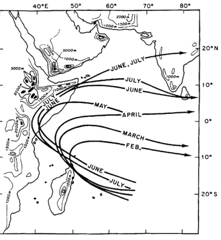
Over the Arabian Sea, which is bounded by the landmasses of East Africa, the Arabian peninsula and the Indian Subcontinent, and the Indian Ocean to the south, this leads to a seasonal cycle of cold, dry northeasterly winds during the winter (NE) monsoon, and warm, moist southwesterly winds during the summer (SW) monsoon. An unique feature of the southwest monsoon over the Arabian Sea is the development of a remarkably strong and steady jet first described by Findlater (1971). The Findlater jet (see Fig. 1.2) is bound in part by the topography of the East African highlands, and the surface winds under the jet in the Arabian Sea are some of the strongest and steadiest in the world (Knox, 1987), with speeds in excess of 15 m sec"1 common.

During the SW monsoon, this strong jet imposes a wind stress curl that leads to Ekman upwelling to the north and west of the jet, off the coast of the Arabian peninsula, and Ekman downwelling to the south and east, in the central Arabian Sea. Hastenrath and Lamb (1979) note Ekman pumping velocities (derived from wind stress curls) implying an upwelling on the order of 1.1 m day- 1 near the Omani coast, and a downwelling on the

(14)

20*N

- _- ₀o

ru 0 M,JUNE

-10

a -20 S

Figure 1.2 The climatological mean of the maximum in the Findlater Jet over the Arabian Sea, and its progression through the monsoon season (from Knox, 1987). upwelling along the southern flank of the Arabian Peninsula. While the NW monsoon does not produce such a strong and well-defined jet, the wind direction is equally steady, and implied Ekman velocities in the central Arabian Sea are about -0.2 m day-1_{. The curl is}

negative, driving downwelling. The general circulation in the Arabian basin is controlled by this seasonal change in Ekman pumping, which also contributes to mixed layer depth.

Climatologies of air-sea fluxes over the Arabian Sea have been hampered by a lack of data, but nonetheless give a general impression of the relevant processes (see Fig. 1.3). At the site of the mooring in the north central Arabian Sea, one climatology (Hastenrath and Lamb, 1979) shows a net heat loss from the ocean during the SW monsoon (which peaks in June and July), thought to be due to a combination of reduced heat losses from cloud

(15)

Climatological wind stress - 15.5 N, 61.5E

0.8 . . . .

Nov Dec Jan Feb Mar Apr May Jun Jul Aug Sep

0.6 Hellermon COADS E 0.4 z 0.2 0.0 300 400 500 600 yearday

Climatological total heat flux

..

I ... I ... I ... I... 300 Nov Dec Jan Feb Mar Apr May Jun Jul Aug Sep

200

(N 100

-100 COADS constrained qtot

COADS raw qtot Wright/Oberhuber

-200 _Hastenrath

l I. . . . . .. . I I

300 400 500 600

yeardoy

Figure 1.3 A summary of the wind stress (top) and total heat flux (bottom) over the Arabian Sea from different climatologies (Hellerman and Rosenstein, 1983; da Silva et al., 1994 (COADS), with heat flux based on the data or constrained so the global net is zero; Wright and Oberhuber, 1988; and Hastenrath and Lamb, 1980). The net oceanic heat gain has a signature twice-yearly cycle. During the NE monsoon (Nov-Dec) the winds are moderate and the ocean loses heat. During the SW monsoon (Jun-Jul) the winds are very strong. From Weller et al. (1997).

(16)

cover and extremely strong winds increasing the latent and sensible heat losses. This has been hypothesized as the driver of the observed twice-yearly cycle of mixed layer deepen-ing and cooldeepen-ing, which is in great contrast to the once-annual cycle typical in midlatitudes (see for example, Martin, 1985). But more recent climatologies (Wright and Oberhuber, 1988; da Silva et al., 1994, see Fig. 1.3), show a net heat gain at the mooring site during the SW monsoon, and demand a different explanation for SW monsoon mixed layer cool-ing and deepencool-ing. By contrast, there is no doubt in the climatologies that the net heat flux is a loss during the NE monsoon, which peaks in December and January, driven by the cool and dry, but only moderately strong winds of the northeast monsoon. These lead to large latent and longwave heat losses, and an overall net heat loss.

The atmospheric forcing of the ocean during each monsoon season can be briefly sum-marized: during the winter NE monsoon, there is a net heat loss, the wind is moderately strong, and the wind stress curl drives a moderate downwelling in the northern part of the Arabian basin. During the summer SW monsoon, the winds are extremely strong and sus-tained, the surface heat gain by the ocean is reduced but positive, and strong wind stress curls drive upwelling in the northern part of the basin and downwelling to the south and east.

1.3 The oceanic response: Arabian Sea circulation and climatology

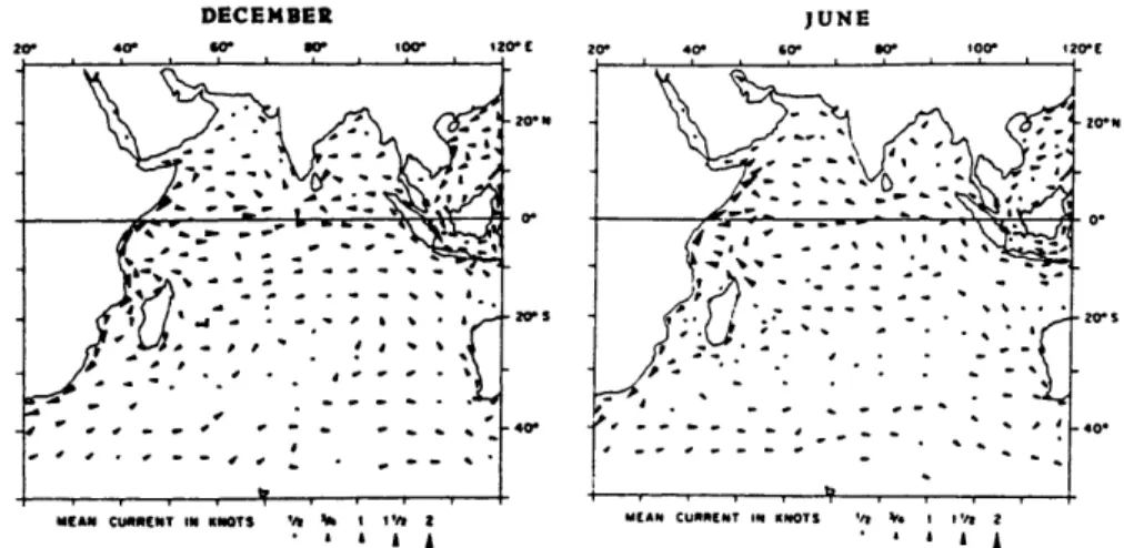
The dramatically changing forcing over the Arabian Sea leads to a dramatic response in the basin's western boundary current, the Somali Current. During the SW monsoon the northward flowing Somali current has a strong transport of 65 Sv, mostly confined to the upper 200 m, and reported currents up to 3.7 m sec- 1 _{(Schott, 1983; Swallow et al. 1983).}

(17)

DECEMBER JUNE

20 40 60 8V to* 20E 20' 40 6 80 100 120* E

20 20"N

\r ,% .."

Figure 1.4 General circulation of the Arabian Sea from shipdrift data, at the height

of the NE monsoon (December) and _{the SW monsoon (June). From Knox (1987)}

(Knox, 1987, see Fig. 1.4). During the SW monsoon, this dynamic current system gives rise to a strong mesoscale eddy field, which has been reported around the basin from the Somali coast to Pakistan (Bruce, 1979; Brown et al., 1980; Evans and Brown, 1981, Bruce and Beatty, 1985; Simmons et al., 1988). The southwesterly winds during the summer monsoon also lead to upwelling along the coast of Oman. The result is persistent jets and squirts of cold, upwelled water which extend from the capes of the Omani coast, often extending far into the interior. These have been observed in satellite SST images, as well as surveyed by SeaSoar (Brink, Lee, Arnone, pers. comm.). During the NE monsoon, Bruce et al. (1994) have reported the persistent formation of a large anticyclonic eddy in the eastern Arabian Sea, with a subsequent westward propagation and decay. The mean current system and in particular the strong mesoscale eddy field, primarily generated dur-ing the SW monsoon, will play an important role in the upper ocean evolution at our site.

While affected by these large-scale circulatory patterns the upper ocean also has a more direct observable response to the wind in the form of Ekman transport convergences and divergences. Especially during the southwest monsoon, the effects of Ekman pumping can be seen in shallow mixed layers, on the order of 20-50m, and high biological

(18)

produc-tivity to the north and west of the Findlater jet (Brock et al., 1992), and in deep mixed lay-ers, up to 100 m, to the south and east (Bauer et al, 1991), with reduced biological productivity. Bauer et al. (1991) found that Ekman pumping plays a first order role in the evolution of the mixed layer and productivity, during both the NE and SW monsoons (see Fig. 1.5).

50"E 60°E 70*E

Figure 1.5 Climatological mixed layer depths in the Arabian Sea during each monsoon, after Rao et al. (1989). The arrow marks the maximum in the wind speed.

Upper ocean transports play an important role in the overall heat balance of the Ara-bian Basin, which reverses seasonally with the monsoon. Diiing and Leetmaa (1980) esti-mated that during the SW monsoon there are three important components to the heat balance: a positive heat gain from the atmosphere, a negative northward heat flux across the equator (in the Somali current), and a heat loss due to upwelling which is the dominant

(19)

term. Hastenrath and Lamb (1979) found that during the SW monsoon the Arabian Sea as a whole gains 0.5 PW of heat from the atmosphere, but loses 0.83 PW due to advection, leading to a net loss. During the NE monsoon, they also found a heat gain of 0.5 PW, of which 2/3 is stored and 1/3 advected out of the basin. In a modeling study by Wacongne and Pacanowski (1996) the Ekman transport played a large role in the meridional heat transport. During the SW monsoon an Ekman transport of 20 Sv across the equator was compensated by a cooler northward deep western boundary current at intermediate depths, implying upwelling as an important driver of the SW monsoon Arabian Sea cooling. Dur-ing the NE monsoon a northward interior flow at the surface was compensated by south-ward deep western boundary currents in the deepest layer. Lee and Marotzke (1997) also found the dominant balance in the north Indian Ocean is between heat storage and heat transport convergences driven by the monsoon. Several layer models of the Arabian Sea and Indian Ocean (McCreary and Kundu, 1989; McCreary et al., 1993) suggest that the process of mixed layer entrainment mediates the large-scale heat balance.

The heat balance in the Arabian Sea has a strong potential for feedbacks with the atmospheric circulation. Because of comparable oceanic and atmospheric timescales in the Arabian Sea, Diiing and Leetmaa (1980) suggested that there might be a feedback between upwelling and the monsoon winds. Gadgil et al. (1984) found in a climatological study that correlations exist between Arabian Sea sea surface temperatures and organized convection over the Indian Ocean, an indicator of rainfall. Studies using general circula-tion models (Kershaw, 1985; Shukla, 1987) have also shown that rainfall over India and the onset of the SW monsoon are affected by sea surface temperature anomalies in the Arabian Sea. In light of these studies, a better understanding of the evolution of the sea surface temperature and the heat content of the upper ocean in the Arabian Sea is a desir-able goal.

(20)

1.4 Objectives

In this thesis, I will focus first on answering some questions that arising from a direct look at the data: Is there net sea surface cooling during the southwest monsoon? What is the dominant physical process causing mixed layer deepening in each monsoon season?

I will then examine what part of the observed upper ocean mixed layer deepening in each monsoon season is locally driven, and what part is nonlocally driven. To clarify these concepts, consider the Reynolds-averaged equation for the evolution of temperature:

aT T a

S +u . VT+ w - (q - ) (1.1)

where T is the local temperature, u is the horizontal velocity vector, V is the horizontal gradient operator, w is the vertical velocity, q is a downwards radiation of heat, and w'T represents a turbulent transport of temperature. I ignore horizontal radiative and turbulent fluxes of heat, which are small compared to other processes in the open ocean. This equa-tion is subject to boundary condiequa-tions at the air-sea interface. Processes defined as local include penetrative solar heating, vertical mixing due to vertical shear-flow instabilities, and surface buoyancy flux-driven convection. In locally-driven processes, the Eulerian temperature evolution aT/t is exactly balanced by the flux terms on the right hand side. Processes defined as nonlocal involve nonzero horizontal or vertical advection terms, and include the obvious horizontal advection of horizontal gradients, as well as vertical advec-tion induced by Ekman pumping or other vertical velocities, like those induced by internal waves, tides, and longer-period waves. Internal waves and tides have periods shorter than the diurnal, and the signal is removed through lowpass filtering.

(21)

Chapter 2 Data and Processing

This thesis focuses on data collected from a surface mooring and subsurface instruments deployed in the Arabian Sea during a full monsoon season. The first two sections of this chapter summarize the collection of the data. The processing used to derive the surface fluxes from the bulk atmospheric measurements is outlined in the third section. And finally, the last two sections give an overview of the surface forcing and the oceanic response at the site through the full monsoonal cycle.

2.1 Mooring Location

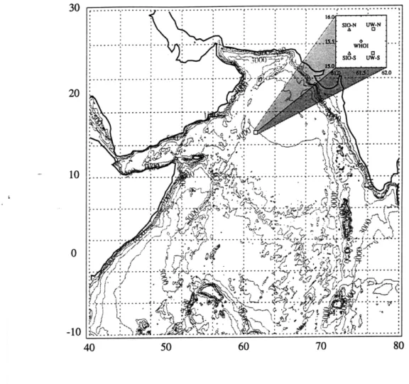
A five-mooring array was deployed in the central Arabian Sea at 61030' E, 15030' N in October 1994 from the Thomas G. Thompson (see Fig. 2.1). The central mooring, the one I focus on primarily, consisted of a surface buoy with a full suite of meteorological mea-surements and subsurface elements. It was recovered and redeployed with new instrumen-tation in the space of 50 hours in April 1995, then finally recovered in October 1995. The two western elements of the array (also recovered and reset after six months) were deployed by D. L. Rudnick, SIO, and consisted of surface buoys supporting a reduced set

(22)

20

... ...--

---40 ... 50 _.- 60 70 80.

contoured in meters. The mooring elements created a square 50 km on a side.

acoustic doppler current profiler (ADCP). The two eastern elements were designed for one-year deployments, came from C. C. Eriksen, UW, and consisted of subsurface

profil-40 50 60 70 80

Figure 2.1 The Arabian Sea with the moored array location. Bathymetry is contoured in meters. The mooring elements created a square 50 km on a side.

of meteorological measurements, subsurface temperature recorders, and one subsurface acoustic doppler curent profickedler (ADCP). The two eastern elements were designcountered for one-year deployments, came from C. C. Eriksen, UW, and consisted of subsurface profil-ing current meters (PCM) which profiled from 30 to 200 m depth. The northern PCM mooring parted and was lost. The deployment lasted through a full seasonal cycle of both the northeast and southwest monsoons.

A location just south of the climatological mean maximum of the Findlater jet during the SW monsoon was picked to maximize the surface forcing that would be encountered.

SIO-N UW-N

WHOI

SIO-S UW-S

(23)

2.2 Instrumentation

The surface element of the central mooring was a 3 m discus buoy, shown in Fig. 2.2. The tower supported two redundant sets of meteorological instruments, one vector-averaging wind recorder (VAWR) and one improved meteorological (IMET) suite. These each mea-sured wind speed and direction at a height of about 3.2 m above the waterline. Each also measured air temperature, relative humidity, and barometric pressure about 2.5 m above the mean waterline. Both measured the incoming shortwave and longwave radiation, and

Figure 2.2 The Arabian Sea mooring surface element, a 3m discus buoy.

Instrumented with two sets of redundant meteorological sensor suites, including wind speed and direction, air temperature, relative humidity, barometric pressure, precipitation, and incoming shortwave and longwave radiation. The buoy also supported a subsurface array or temperature sensors attached to the buoy bridle.

(24)

the IMET package included a precipitation gauge. An aspirated air temperature sensor was also included to investigate daytime radiative heating errors. Due to power limitations, aspiration stopped part way through each deployment, but an algorithm developed using the data that was collected (Anderson and Baumgartner, 1997) to correct the naturally aspirated sensors for radiative heating is applied here.

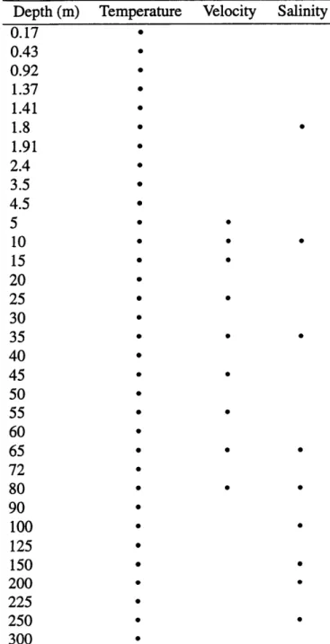
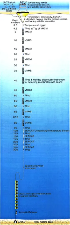
The subsurface instrumentation on the central mooring measured temperature, veloc-ity and salinveloc-ity in the upper 300 m. Instrumentation included vector-measuring current meters (VMCM), moored CTDs (Seacats), temperature sensors (TPods), and multi-vari-able moored sensors (MVMS, from T. Dickey and J. Marra) which measured temperature, velocity, and salinity. A summary is given in Table 2.1 and Fig. 2.3. Subsequent analysis of SeaSoar data (Lee, pers. comm.) showed that large salinity inversions, generally density compensated, existed in the thermocline, which were not resolved by the spacing of the salinity sensors on the mooring. The temperature sensors provided good resolution of both the mixed layer and the main thermocline. The velocity measurements provided good cov-erage of the mixed layer for all of the deployment except for when the mixed layer was at its deepest, during the northeast monsoon.

Each instrument was calibrated before and after its six-month deployment. The esti-mated error in each measurement is detailed in Table 2.2. These estimates are based on calibrations, as well as intercomparisons made with the same instruments in previous experiments (Weller and Anderson, 1996). They are given for instantaneous values, although they are generally better at night when radiative heating does not compromise the sensors.

(25)

Table 2.1: Subsurface instrumentation on the central mooring. Temperature * * * * * * * Velocity Salinity (m) ~ IliL'' ~~""'~~~~~~ Depth 0.17 0.43 0.92 1.37 1.41 1.8 1.91 2.4 3.5 4.5 5 10 15 20 25 30 35 40 45 50 55 60 65 72 80 90 100 125 150 200 225 250 300

(26)

dissolved oxygen, and line tension sensors, inDepthrs and backup satellite transmitter

3.5 t Temperature Logger 4.5 TPod at Top of VMCM 5 VMCM 10 MVMS 15 VMCM 20 TPod 25 VMCM 30 sTPod 35 MVMS

40 TPod & Holliday bioacoustic instrument

for detecting zooplankton with sound

45 VMCM

so TPod

55 VMCM

,,r -f Anchotr -.- 4032 meters dp

Figure 2.3 A schematic of the subsurface elements on the Arabian Sea mooring. The upper 300m had multiple instruments measuring temperature, salinity, and velocity, as well as a variety of bio-optical parameters, not discussed here.

(27)

Table 2.2: Estimated accuracy of measurements. Variable Instantaneous accuracy

wind speed 5 %

wind direction 10 0 barometric pressure 0.5 mb air temperature 0.2 oC

sea surface temperature 0.1 oC incoming shortwave 3 % incoming longwave 10 W m-2 relative humidity 4 % subsurface temperature 0.01 OC subsurface salinity 0.01 psu subsurface velocity 1 cm sec- 1

2.3 Bulk calculation of air-sea fluxes

The air-sea fluxes of heat, momentum, and freshwater are calculated with a bulk formula-tion, since these fluxes are not measured directly. Here the formulation developed for the TOGA COARE experiment (see Fairall et al., 1996a) is used, which is valid under a large variety of forcing conditions. The essentials of the bulk flux formulation and Fairall et al.'s method are described below. The accuracy of the computed fluxes is presented in the last section below.

The net heat flux across the air-sea interface is computed as the sum of four compo-nents: the net shortwave radiation absorbed by the ocean, the net longwave heat loss due to radiation, the latent heat flux due to evaporation, and the sensible heat flux. The time series of these components is presented in Fig. 2.5.

(28)

Qsw = (1 - as) SW$

where as is the albedo of the sea surface, calculated according to Payne's (1972) algo-rithm, and has a nominal value of 0.06. The daily peak in the net shortwave heat flux was quite strong, about 1000 W m-2, although the daily average varied seasonally from about 200 W m- 2 to 300 W m-2, with two yearly peaks due to the location in the tropics. Values

were reduced during the cloud cover of the SW monsoon, and the deployment average was 243 W m-2.

Incoming longwave radiation from atmospheric water vapor and clouds is measured on the buoy. The net longwave heat transfer across the air-sea interface is the sum of this measured incoming LW radiation and the outgoing radiation from the sea surface. The sea surface is assumed to radiate as a gray body, so the net longwave heat flux is

QLW = LW--essaTs kin- (1 -ss)LW (2.2)

where ess is the longwave emissivity of the sea surface, taken to be 0.97, a is the Stefan-Boltzmann constant, Tskin is the sea surface skin temperature (computed according to Fairall et al.'s (1996b) warm layer/cool skin algorithm; more about this below), and the albedo of the sea surface is taken as one minus the emissivity. The net longwave heat loss from the sea surface was generally on the order of -60 W m-2, but was greatly reduced dur-ing the cloud cover of the SW monsoon. The deployment average was -58 W m2_.

The latent heat flux is due to the evaporation of water off the sea surface. The turbulent latent heat flux is defined by the Reynolds average, and is Qlat = PaLw'q', where pa is

the density of air, L, is the latent heat of vaporization, w' and q' represent turbulent fluc-tuations of vertical velocity and specific humidity, and the overbar denotes a time average. The bulk representation is:

(29)

Qlat

= PaLvCeUw (qs - q)

where ce is the latent heat transfer coefficient, uw is the average wind at the reference

height, and qs is the saturation specific humidity at the air-sea interface. The latent heat transfer coefficient is a nonlinear and semi-empirical function of the wind speed, atmo-spheric stability, surface roughness, and measurement height, and is computed using the Fairall et al. (1996a) algorithm. The latent heat flux was strong during the NE monsoon, on the order of -200 W m-2 _{due to reasonable winds and low relative humidity, but despite}

stronger winds it was reduced during the SW monsoon as the air became saturated, rang-ing between -50 and -150 W m-2. The deployment average was -122 W m-2_.

The sensible heat flux, due to direct conduction of heat from the atmosphere into the ocean, can be written in turbulent flux form as Qsens = PaCpaW'T , where Cpa is the heat

capacity of air, and T represents a turbulent fluctuation of temperature. The bulk repre-sentation is

Qsens = PaCpaChlUwl(Tskin - 0) (2.4)

where ch is the sensible heat transfer coefficient and 0 is the potential temperature of the air directly above the interface, corrected for reference height. The Fairall et al. (1996a,

1996b) algorithm again estimates the transfer coefficient, as well as the skin temperature of the ocean. The sensible heat flux ranged from values of about -10 W m72_{, during the NE}

monsoon as cooler continental air flowed over the ocean, to about +10 W m- 2 during the

SW monsoon, as warm oceanic air passed over a newly entrained, cooler sea surface. The average over the deployment was -1.5 W m-2.

The net heat flux is then the sum of these components,

Qnet = Qsw + Qlw + Qlat + Qsens. (2.5)

_IIIII_ 1L(li..~~----~ ~-~I.~~~

(30)

There is an additional effect due to the heat flux of rainfall, but this is neglected here (although not in the freshwater budget) since the rainfall amount was so small. Daily aver-ages of the net heat flux varied between about -200 W m-2 and +250 W m-2_{, although the}

balance was strongly towards an oceanic heat gain, with a deployment average of +61 W m-2.

The wind stress exerted at the air-sea interface can be written in turbulent form,

t = PaW'Uw', where u_w' _{is a turbulent fluctuation of the magnitude of the horizontal}

wind. The bulk formulation is

T = PaCdUwiUw[ (2.6)

where cd is the stress transfer coefficient, also known as the drag coefficient. In this case, and in all cases above, u_w_{refers to the wind speed at the reference height with respect to}

the surface current. The VMCM measured velocity at 5 m was subtracted from all wind measurements. The drag coefficient was again calculated using the TOGA COARE bulk flux algorithm. During the NE monsoon, daily averaged values of the wind stress ranged from 0.1 to 0.2 N m-2, while during the SW monsoon they peaked as high as 0.6 N m-2. The deployment average was 0.1 N m-2

The freshwater flux through the air-sea interface is the difference between a gain through precipitation, which was measured directly, and a loss through evaporation. The evaporative loss is calculated from the latent heat flux, and is

E at (2.7)

PoL,

where po is the density of seawater and the latent heat of vaporization L_vis taken to be a constant 2.434 x 106 J kg-1._{The freshwater flux is then just E}_- _{P, expressed as a}

(31)

veloc-ity.

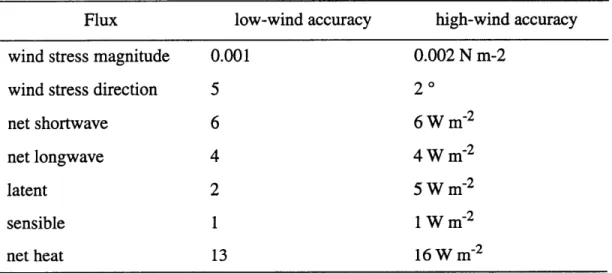
The Fairall et al. (1996a) bulk flux algorithm was developed and tuned through direct comparisons with inertial-dissipation methods of measuring fluxes in the warm pool region of the equatorial Pacific. Weller and Anderson (1996) reported conditions during TOGA COARE with wind speeds that range from 0.01 - 17.17 m sec-1, comparing favor-ably with the 0.04 - 18.34 m sec- 1 recorded in the Arabian Sea, and similar ranges in air temperature and relative humidity. The largest difference in ranges come from the SST. Weller and Anderson computed estimates of month-long accuracies in the air-sea fluxes for low wind and high wind situations, reported in Table 2.3, adjusted for the level of cali-brations and intercomparisons used in this experiment.

Table 2.3: Estimates of the month-long accuracy in the calculated air-sea fluxes, after Weller and Anderson (1996).

Flux low-wind accuracy high-wind accuracy wind stress magnitude 0.001 0.002 N m-2

wind stress direction 5 2 o

net shortwave 6 6 W m-2

net longwave 4 4 W m-2

latent 2 5 W m- 2

sensible 1 1 W m-2

net heat 13 16 W m-2

2.4 Overview of Atmospheric data

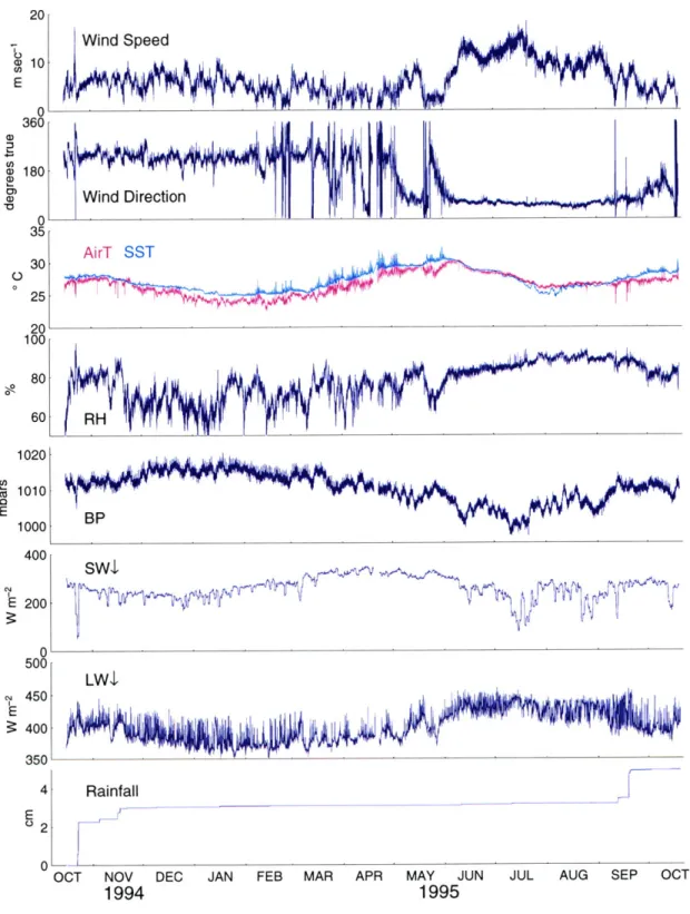
The measured atmospheric data is shown in Fig. 2.4, and the record is dominated by the signal of the two monsoon seasons, each with dramatically different forcing.

The mooring was deployed not long before the start of the winter northeast monsoon. After an initial storm in late October, which is noted by spikes in the wind speed,

(32)

JAN FEB MAR APR MAY JUN

1995

JUL AUG SEP OCT

Figure 2.4 The measured meteorological variables for the full deployment of the Arabian Sea surface mooring. From top to bottom: first, the wind speed and direction, then air temperature (after correction for radiative heating) and sea surface temperature (at 17 cm depth). Then the relative humidity, barometric pressure, daily-averaged incoming shortwave radiation, incoming longwave radiation, and cumulative rainfall.

Wind Speed 1020 1010 1000 400 E 200 0-500 S450 S400 4 E 02 0-BP Rainfall I Y OCT NOV 1994 DEC

0?0

(33)

-ity, barometric pressure, solar radiation, and rainfall records, the first few months of the deployment are dominated by the NE monsoon. The wind speeds during this period, which extends roughly from October 1994 through January 1995 at the mooring site, were moderately strong, ranging from about 5 - 10 m secl1. But they were not completely steady, showing a modulation, with periods of higher winds lasting about five days appear-ing approximately every 15-20 days. The direction, which marks the monsoon seasons well, was very steady and from the northeast, with a mean true direction of 226 degrees. During this period, the relative humidity was fairly low and the barometric pressure high, indicative of drier continental air being forced off the Asian continent. The air temperature and sea surface temperature both dropped during this period, although SST remained higher than the air temperature throughout. The slightly reduced levels of incoming solar radiation are due primarily to reduced levels of insolation in the winter season, rather than cloud cover. And finally, the reduced levels of downwelling longwave radiation are in keeping with the low cloud cover and relatively low moisture the atmosphere.

From February through May 1995, intermonsoon conditions predominated. The wind speed reduced and wind direction shows variations that tend to remain on the northeast-southwest axis, but exhibit clockwise rotations due to low pressure systems to the south, which generally move westward (Kindle, pers. comm.). The air temperature and sea sur-face temperature both climb during this period, with evidence of strong diurnal heating.

The southwest monsoon dominates the record from May through the end of September 1995, although the start date of the SW monsoon is difficult to pin down. Certainly at the beginning of May the stronger (up to 10 m sec- 1) and steady southwesterly direction of the

winds, along with increased humidity, would indicate a beginning of the monsoon, but it appears to falter for the first week of June. By the second week of June, however, the southwest monsoon has reestablished itself, and does not relinquish its hold until the end

(34)

of September. Wind speeds are strong, ranging from 10-15 m sec- 1_{, with gusts up to 18}

m sec- 1_{. The direction is extremely steady from the southwest, with a mean true direction}

of 52 degrees. The air temperature and sea surface temperature again diminish, although this time the sea surface is for the most part cooler than the air temperature. The relative humidity is very high, hovering near 90%, and the barometric pressure is reduced, consis-tent with maritime air being pulled towards the Asian continent. The incoming solar radia-tion record is sharply reduced, in part due to the natural yearly cycle which has two peaks in the tropics, but primarily showing the strong influence of clouds (Weller et al., 1997). The high levels of moisture in the atmosphere are further reflected in the high levels of incoming longwave radiation. Precipitation during this period at the site is negligible.

The record ends going into another intermonsoon period, as the winds relax, and the air and sea surface temperature recover somewhat before the start of a new cycle.

The computed air-sea fluxes of heat and momentum are shown as daily averages in Fig. 2.5. During the northeast monsoon, a combination of factors led to a net heat loss from the ocean. The strongest latent heat losses of the deployment are observed during this period, driven by the moderate flow of dry air over the sea surface. The sensible heat loss, while small as always contributes to this heat loss as the ocean is warmer than the cold continental air. The net shortwave heat flux is weak, due to reduced winter insolation. And the net longwave heat flux remains strong as there is little moisture in the atmosphere to reduce it. The heat loss is modulated by the characteristic modulation of the wind speed. This can also clearly be seen in the wind stress record, as broad peaks of wind stress approaching 0.2 N m-2 _{are followed by periods of reduced wind stress.}

As mentioned before, a net heat loss at this site has been reported during the southwest monsoon (Hastenrath and Lamb, 1979), although this is disputed by other climatologies. The record shows that at the mooring site, the net heat flux stays positive for the large

(35)

-50 -100 0 -100 E -200 -300 -400 20 10 0 -10 -20 200 100 0 -100 -200 QLW

OCT NOV DEC JAN FEB MAR APR MAY JUN JUL AUG SEP OCT

1994 1995

Figure 2.5 The calculated air-sea fluxes of momentum and heat at the Arabian Sea mooring site for the entire deployment. From top to bottom: the wind stress, the net shortwave heat flux, the net longwave heat flux, the latent heat flux, the sensible heat flux, and finally the total heat flux. All have been passed through a daily running average.

, V

(36)

majority of the southwest monsoon. Despite extremely strong winds, the latent heat loss is quite low due to the high humidity of the air. While cloud cover does lead to a reduced shortwave heat flux, the net longwave heat flux is held very low due again to the high atmospheric water vapor content. With a sensible heat flux now reversed due to the rever-sal in the air-sea temperature gradient, the net heat flux is primarily positive, with only two short periods of reversal in the daily average. The average heat flux over the whole SW monsoon period (May-September) is 62 W m-2 _{into the ocean.}

2.5 Overview of Oceanic response

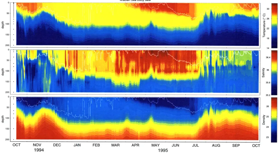
The subsurface record of temperature, salinity, and density during the full year deploy-ment is presented in Fig. 2.6. Like the atmospheric record, it is dominated by the signal of the two monsoon seasons. Unlike the atmospheric record, the primary manifestation of the monsoon, a cooling and deepening of the mixed layer, is very similar in each season.

The dominant signal in the mixed layer depth record is the twice-annual cycle of deep-ening and shoaling. During the NE monsoon, which peaks in November, December and January, the mixed layer, at least as defined by temperature, deepens from approximately 20 m to a maximum of nearly 100 m. As the winds die down and the net heat flux reverses sign into January, the mixed layer begins to shoal quickly, as the upper water column restratifies. The residual deep mixed layer is left behind, underneath the newly formed mixed layer. During the intermonsoon season the mixed layer remains shallow as weak winds and a strong positive heat flux strongly stratify the upper part of the water column. When the SW monsoon picks up in June, the mixed layer again deepens, this time only reaching a maximum depth of about 75 m. Although winds continue to blow strongly, the mixed layer shoals slowly through the end of July and into August in an advective event.

(37)

Arabian Sea Buoy data 0 S26 ~100 a Cz *0 f22 E 150 a 18 200 14 i i 36.4 150 150 ~3635.6 200 2000 35.2 26 100 24 150 23 200

OCT NOV DEC JAN FEB MAR APR MAY JUN JUL AUG SEP OCT

1994 1995

Figure 2.6 The upper ocean in the Arabian Sea. Contours of (from top): temperature, salinity, and density anomaly as they

evolved in time, lowpass filtered to remove the tides. The mixed layer, as defined by a 0. 1C difference from the SST, is plotted in white. Dots at left indicate sensor depths.

(38)

Intermonsoon conditions return in September, and the mixed layer remains shallow for the rest of the deployment.

The temperature of the mixed layer cools during each monsoon season as the mixed layer deepens. During each intermonsoon period, as the water column restratifies and the mixed layer remains shallow, the temperature climbs. The subsurface temperature gradi-ent, which dominates the calculation of density, shows a remarkable vertical migration throughout the year. During the mixed layer deepening phase of the NE monsoon, the thermocline deepens, in concert with the base of the mixed layer. It remains deep, without much apparent vertical motion, through the intermonsoon leading into the SW monsoon. It does not move as the SW monsoon mixed layer deepens, but does migrate upwards, concurrent with the mixed layer shoaling at the end of July and into August.

The salinity signal is marked by patchiness, following the small horizontal and vertical scale over which salinity varies. The sensor spacing does not fully resolve all the structure in the salinity. The mean conditions over the year are strongly evaporative, and the salinity of the mixed layer does generally increase through the NE monsoon, the intermonsoon, and into the SW monsoon. Then an abrupt freshening of the mixed layer occurs, concur-rent with the slow shoaling of both the mixed layer and the thermocline. The density sig-nal is largely dependent on the temperature, and follows a similar evolution.

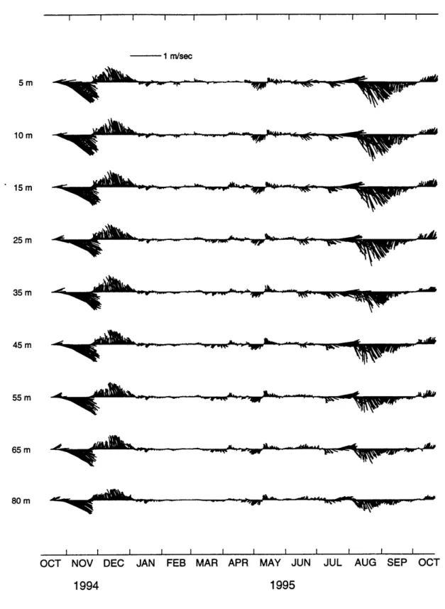
The subsurface velocity record is presented in Fig. 2.7 and in Fig. 2.8. The general velocities are quite strong, of the order of 1 m sec- 1 during the NE monsoon and in the

lat-ter half of the SW monsoon. The strongest velocities are roughly correlated with the observed changes in the thermocline depth, suggesting that these could be the result of horizontal advection of gradients.The velocities in the NE monsoon are remarkably coher-ent throughout the water column, largely not the local response to the wind, but a velocity mode that is nearly barotropic. Intermonsoon periods have much smaller velocities in

(39)

gen-5m 10 m 15 m 25 m 35 m 45 m 55 m 65 m 80 m 1994 1995

Figure 2.7 The velocity record in the upper ocean as stickplots. North is up, and velocities have been daily averaged.

I I I I I I I I I I I

1 m/sec

-*A-I I I I I I I I I I I I

(40)

I I | I I I I I I I I I - 10 cm/sec 301.2 m 492 m 749.5 m I _ .' -I I I I I I I I I I I I

OCT NOV DEC JAN FEB MAR APR MA9 UN JUL AUG SEP OCT

Figure 2.8 The deep velocity record as a stickplot. North is up. These VMCMs were placed on the UW-S mooring.

eral. The velocity during the SW monsoon is more depth dependent than that observed during the NE monsoon, implying that a larger part of it is the local response to the wind. But again, the strongest velocities are tied to the biggest changes in the water column, in August.

Our task is now to examine in further detail the deepening and cooling seasons of the mixed layer responding to the NE and SW monsoons.

(41)

Chapter 3 Northeast Monsoon

The northeast, or winter, monsoon is in some ways the more quiescent of the two. The winds are quite steady in direction, but are moderate. The winter Asian landmass is the progenitor of what the winds carry: relatively cool and dry air. Without an insulating blan-ket of atmospheric moisture the longwave heat loss at the sea surface is high, and the latent heat loss is large as evaporation reaches is at its yearly peak. This makes the overall net heat flux across the air-sea boundary destabilizing in the ocean, and combined with the addition of a salt flux into the ocean, the daily average of the buoyancy flux is always destabilizing.

The aim here is to look at the observed deepening and cooling of the upper ocean dur-ing the northeast monsoon, and determine what physical processes, local and nonlocal, are primarily responsible. A six week period of the year-long time series is extracted and examined in isolation. This is a period of characteristic northeast monsoon forcing, and the period over which the majority of the deepening occurs. The approach will be to run a series of tests, first to determine the dominant local mechanism driving deepening, then to test the idea that the upper ocean evolution is a local response to the local surface forcing.

(42)

Other mechanisms of upper ocean forcing which have been postulated to be important include vertical motions due to Ekman pumping and other vertical velocities and horizon-tal advection of gradients in properties. The first section of this chapter frames the upper ocean in its larger-scale oceanic background. The next two sections examine the local forcing and characterize the upper ocean response. Then the dominant local mechanism for deepening is examined through a look at the surface forcing. The impact of local and nonlocal processes are then analyzed through budgets and one-dimensional modeling. Finally the results are summarized in the last section. One finds that although the upper ocean evolution is not entirely inconsistent with a local response, horizontal advection is crucial in understanding the mixed layer depth evolution. The primary role that horizontal advection plays here is not in direct fluxes of heat and salt into the mixed layer, but in advecting a changing mixed layer depth past the site.

Strict monsoon seasons are difficult to define, although perhaps the clearest indication is the steadiness in the direction of the wind. By that definition (see Fig. 2.4), the northeast monsoon would extend from the last week of October through mid-January. Since my interest here is in the deepening and cooling of the mixed layer in response to the mon-soon, I restrict my view to a shorter period of time which encompasses the majority of this response. In mid-November, the sea surface temperature (SST) has already cooled slightly to 27.5 'C from the deployment SST of 28 'C. But a sustained temperature drop to 25.5 'C occurs through the beginning of January, at which point the SST levels off and slowly begins to climb again. The mixed layer depth, as defined by a 0.1 'C difference from the SST, is relatively shallow in mid-November, with diurnal stratification reaching to within a few meters of the surface and nighttime values of the mixed layer depth around 30 m (see Fig. 2.6). By the beginning of January, the mixed layer has reached its northeast monsoon maximum depth of just under 100 m, and after this periods of shallow diurnal stratification

(43)

become more frequent and last longer, decreasing the mean mixed layer depth. To exam-ine this period of deepening and cooling, I extract a six week period extending from November 20 through January 1.

3.1 Oceanographic setting

The northeast monsoon shares with the southwest monsoon the broad scale of forcing over the Arabian Sea, although the strength of the momentum forcing is much reduced. The mesoscale activity in the basin is largely generated during the more energetic SW mon-soon (Kantha, pers. comm.), and the broad even forcing of the NE monmon-soon, including a diurnal restratification, appears to horizontally homogenize the mixed layer, reducing hor-izontal SST gradients. Satellite AVHRR imagery of the sea surface (Arnone, pers. comm.) shows broad horizontal homogeneity at the surface in the NE monsoon. A SeaSoar survey (Brink, Lee, pers. comm.) in September-October also revealed broad horizontal homoge-neity in the mixed layer in a line extending from the Omani coast southeast past the moor-ing site into the central Arabian Sea. Before the moormoor-ings were set in October 1994, shortly before the NE monsoon season, an extensive XBT survey, covering a diamond-shaped pattern 100 km by 100 km centered on the mooring site, revealed near-homogene-ity in the horizontal direction at depths up to 300 m. Observed gradients were smaller than 0.01 °C/km. While the mixed layer appeared to be horizontally homogeneous, the rem-nants of the previous season's SW monsoon eddy activity were evident, noted as large ver-tical excursions in the thermocline in the SeaSoar data, and as sea surface height anomalies in TOPEX data.

An estimation of the horizontal gradient in temperature made possible by the data from the mooring array reveals that the horizontal homogeneity in the mixed layer was

(44)

maintained during the period on which I focus. To generate this estimate, data from three moorings, the central WHOI mooring, and the two SIO moorings (see Fig. 2.1), were used. Temperature and velocity data at each mooring were 48-hour lowpass filtered to remove signals at tidal and inertial frequencies. Salinity was not available on the SIO moorings. Since the moorings record data for all spatial scales, including those not resolved by the array, an EOF decomposition for the specified time period was made, after which the data was represented in a truncated EOF expansion, only retaining the most dominant modes to capture the signal coherent across the array (following the technique of Rudnick et al., 1993). In temperature, the first four EOFs were retained, accounting for 98.7% of the variability in the lowpass filtered fields. In velocity, only the first two EOFs were retained, for 95.4% of the variability. The temperature data at each mooring was spline fitted onto a 5 m resolution vertical grid common to all three moorings, and the

0

10

120

26 D2c 8 14 20 26 1

SDec Jan

upstream grad T (oC/km)

-0.03 -0.02 -0.01 0 0.01 0.02 0.03

Figure 3.1 The upstream gradient in temperature based on the mooring array data. A positive gradient indicates warming. Mixed layer depth (blue) based on lowpass filtered temperature data. The upstream direction below 80 m is represented only by the two SIO moorings.

(45)

average temperature and temperature gradients for the array were estimated using a simple plane fit at each depth. The gradient was projected onto the upstream direction, with veloc-ity taken as the array average in a similar manner to the temperature. The result (Fig. 3.1) shows small horizontal gradients within the mixed layer, but large gradients below, consis-tent with the homogeneous mixed layer but horizontally varying thermocline noted in ear-lier. 1000 5 25 _(a) (b) 800 200 s 600 0 0 - "100 , S400 . . .E 56 200 0 0 -600 -400 -200 0 200 400 -100 0 100 km east km east M raw ₂₀₀ (c) (d) Mek 0 • -200 -100 0 km east

Figure 3.2 Progressive vector diagrams and the Ekman transport relation for the NE monsoon. Dots are separated by six days. (a) The raw velocities seen at the mooring, (b) the same as (a) with the 80 m velocity subtracted, (d) velocities from a one-dimensional PWP model run, (c) The observed transport integrated over the time period to a depth of 80 m (Mraw), with the 80 m velocity removed (Mup), and as expected from the mean wind stress (MEk). The mean wind stress is t.

(46)

The velocities recorded at the WHOI mooring during the NE monsoon are quite large, and represent far more than a local response to the wind forcing. A progressive vector dia-gram of the velocity, and the velocity with the deepest (80 m) upper ocean velocity removed (see Fig. 3.2), indicates that the local response is only a small fraction of the total measured response. The figure also shows the results of a one-dimensional model forced with the given surface conditions (see Section 3.5.3), the captured transport in the observa-tions, and that expected from Ekman theory. They all show that the observed velocity in the upper ocean is very much larger than that expected from a local balance.

Since the velocity term is very large, one might expect the horizontal advection of properties to be important in the evolution of the mixed layer and the upper ocean. But since the horizontal gradient in temperature has been shown to be very small, a one-dimensional evolution equation will still perform adequately in predicting the evolution of the mixed layer temperature, although it will miss important details in the mixed layer depth evolution.

3.2 Surface Forcing

The surface fluxes of momentum, freshwater, and heat are shown in Fig. 3.3. The wind stress is moderate but variable, with an average of 0.08 and standard deviation of 0.04 N m-2_{. Reflecting the low relative humidity and moderately strong winds, evaporation is} quite strong, with no precipitation to balance it. The mean evaporative rate is 6.6 mm day-l _{. The net heat flux changes sign daily as the incoming solar radiation dominates}

over surface heat losses, with a peak gain of 762 W m-2 _{and a maximum loss at night of}

(47)

0.25 0.2 0.15 0.1 -0.05 1.5 C 0.5 S ₁₀₀oo -500 20 26 2 8 14 20 26 1

Nov Dec Jan

Figure 3.3 Timeseries of the surface forcing during the northeast monsoon. From top: the wind stress, the latent heat flux, the net heat flux, fully resolved and daily averaged.

represents an oceanic heat loss. A one-day running average shows that for the majority of the time during this six-week period the net heat flux is destabilizing.

The surface buoyancy flux is critical in terms of predicting the presence of penetrative convection and the ensuing entrainment at the base of the mixed layer. It is defined here, with units of kg sec-1 m-2, as

B = po[a(poCp) Qnet- S(E - P)] (3.1)

where a and p are the respective coefficients of expansion due to temperature and salt, assumed constant, So is an average surface salinity, and the average surface density po

and heat capacity Cp were diagnosed from mean upper ocean values of the temperature

(48)

xl 10 -5 -10 -15 -20 . . . . 20 26 2 8 14 20 26 1

Nov Dec Jan

Figure 3.4 The daily average surface buoyancy flux, total (thick line), due to the heat flux (thin line), and due to the freshwater flux (dotted line).

and salinity. A positive buoyancy flux is stabilizing. The timeseries of the buoyancy flux is shown in Fig. 3.4. It is destabilizing on a diurnal timescale during nearly all of this record. The largest destabilizing flux occurs towards the end of the record, modulated by pulses in the wind speed which lead to large latent heat losses.

The spectra of the surface forcing are shown in Fig. 3.5. The net heat flux has a strong peak corresponding to a period of 24 hours, along with harmonics at shorter periods. The other fluxes are generally red, with a mild peak noted at the diurnal period in the clock-wise-rotating component of the wind stress.

During this period, the primary local driving mechanism would appear to be the strong, steady, and destabilizing buoyancy flux. This should erode the stable stratification below the mixed layer, entraining cooler and fresher water and deepening the mixed layer. The strength of the wind stress and its ability to cause shear-driven instabilities and verti-cal mixing at the mixed layer base should not be discounted, however, as the forcing is moderate in strength. The dominant local forcing will be examined below.

(49)

10-2 cpd 10-0.001 0.01 0.1 1 10 cph 10 102 Qnet Qlat 106 106 -CL 10' 10' 102 cpd 10 cpd 0.001 0.01 0.1 1 10 0.001 0.01 0.1 1 10 cph cph

Figure 3.5 Autospectra of the surface forcing for the NE monsoon: wind stress r, net heat flux Qnet, and evaporative heat flux Qlat. The rotary autospectra is shown for the wind stress, and a frequency of one cycle per day (cpd) is marked.

3.3 Characterizing the upper ocean response

The upper ocean response during this six-week period of characteristic northeast monsoon forcing is not immediately inconsistent with a local response to the local forcing: the mixed layer deepens and cools and the sea surface salinity slowly increases. But we shall see that nonlocal processes will have to be called into play to explain the extreme depth of the mixed layer penetration.

(50)

pp

~7r~ rh 50U E 10 150 200 0 50 - 100 0o 150 200 0 50 - 100 V, 200 20 26 2 8 14 20 26 1 Dec Jar

Figure 3.6 The lowpass-filtered subsurface temperature, salinity, and density. Dots at the left margin show the heights of the

measurements. The mixed layer (displayed as a line, unfiltered) deepens and cools during this period. Salinity shows marked signs of variability. 30 26 I-18 14 36.4 36 35 35.6 35.2 O3 24 111111111)11 -0