Analyzing cities' complex socioeconomic networks using computational science and machine learning

(1)

Analyzing Cities' Complex Socioeconomic Networks

Using Computational Science and Machine Learning

by

Ahmad Alabdulkareem

M.S. in Computer Science, King Abdullah University for Science & Technology (KAUST), 2011

B.S. in Computer Science, King Saud University, 2010 Submitted to the Center for Computational Engineering and to the Department of Civil and Environmental Engineering

in partial fulfillment of the requirements for the degree of

Doctor of Philosophy in Computational Science & Engineering at the

MASSACHUSETTS INSTITUTE OF TECHNOLOGY

June 2018

@

Signature redacted

A u th o r ... .. ... .... ... ... ... ... ... .. .. ... .. .. ... .... ... ... ... .. .

Center for Computational Engineering

~)D y ~ay'd 2018

Signature redacted

Certified by...

Certified by ...

...Ir ...0 , . ...

Alex "Sandy" Pentland

Toshiba Professor of Media Arts and Sciences

Tlesis Supervisor

Signature redacted...

- --- John R. Williams Professor of Information Engineering

//

Thgsis Supervisor

Signature redacted

A ccepted by...

PJesse Kroll

Professor of Civil and Environmental Engineering Chair, Gradyae-Vrogram Committee

Signature redacted

Accepted by...

- icoTas Hadjic ou

Co-Director, Computational ngineering MASSACHUSETTS INSTTTE

OF TECHNOWGY

JUL 26 2018

(2)

(3)

Analyzing Cities' Complex Socioeconomic Networks Using

Computational Science and Machine Learning

by

Ahmad Alabdulkareem

Submitted to the Center for Computational Engineering and to the Department of Civil and Environmental Engineering

on May 18, 2018, in partial fulfillment of the requirements for the degree of

Doctor of Philosophy in Computational Science & Engineering

Abstract

By 2050, it is expected that 66% of the world population will be living in cities. The

urban growth explosion in recent decades has raised many questions concerning the evolutionary advantages of urbanism, with several theories delving into the multitude of benefits of such efficient systems. This thesis focuses on one important aspect of cities: their social dimension, and in particular, the social aspect of their complex socioeconomic fabric (e.g. labor markets and social networks). Economic inequality is one of the greatest challenges facing society today, in tandem with the eminent impact of automation, which can exacerbate this issue. The social dimension plays a significant role in both, with many hypothesizing that social skills will be the last bastion of differentiation between humans and machines, and thus, jobs will become mostly dominated by social skills. Using data-driven tools from network science, ma-chine learning, and computational science, the first question I aim to answer is the following: what role do social skills play in today's labor markets on both a micro and macro scale (e.g. individuals and cities)? Second, how could the effects of automation lead to various labor dynamics, and what role would social skills play in combating those effects? Specifically, what are social skills' relation to career mobility? Which would inform strategies to mitigate the negative effects of automation and off-shoring on employment. Third, given the importance of the social dimension in cities, what theoretical model can explain such results, and what are its consequences? Finally, given the vulnerabilities for invading individuals' privacy, as demonstrated in previ-ous chapters, how does highlighting those results affect people's interest in privacy preservation, and what are some possible solutions to combat this issue?

Thesis Supervisor: Alex "Sandy" Pentland

(4)

Thesis Supervisor: John R. Williams

(5)

Acknowledgments

This is without a doubt the hardest part to write in my entire thesis, and I am fighting the urge to make it longer than the thesis itself, because I know I cannot do justice to everyone who supported and encouraged me. Therefore, I will force myself to restrict this to two pages.

I am grateful to all of the amazing members of my committee. I was extremely

lucky to have such an impressive set of professors guiding me. Starting with the person who had the biggest influence on my PhD, I want to thank someone who was more than just an advisor: my friend, Professor Alex "Sandy" Pentland. He not only provided me feedback and assistance in my research, but has also made sure to help me in my personal life and future career. This brings me to the person who introduced me to Sandy many years ago, Professor John R. Williams, who was my guide in both life and academia alike. I still fondly remember our long talks when I first came to Boston almost a decade ago. I was also fortunate to work with Professor Iyad Rahwan, who was kind enough to welcome me into his group. He never asked what was in it for him, and he greatly helped me in my research when the time came. Finally, I want to thank Professor Marta Gonzalez, the ace in my committee. Whenever I ran into a roadblock, Marta was always there to walk me through it, always asking thought-provoking questions to help me advance my work.

This brings me to Professor Anas Alfaris, who I would call my father figure if he did not hate that for making him sound old, since he is not that much older than me. As such, I will stick to calling him my very close friend. Anas was my first real mentor. He taught me the skills I needed to succeed in life, and then some. I can, without any doubt in my mind, say that I would not be where I am today without him.

I appreciate all of the various groups' very supportive staff, who were always extremely helpful, especially Kate Nelson and Kiley Clapper. To all of my many colleagues and amazing friends at the Center for Complex Engineering Systems, thank you. To my fellowship sponsor, King Abdulaziz City for Science and Technology, I

(6)

really appreciate your generous support, especially from CCES's deputy director, Adnan Alsaati, and KACST's president, HH Dr. Turki Al Saud. I am truly fortunate to come from a country that supports education in every way possible.

I was blessed to have made many friends during my PhD. Unfortunately, I cannot

list them all, though they are an integral part of who I am. I would like to send a hearty shout-out to all of the members of the Human Dynamics (especially Abdul-rahman Alotaibi), Scalable Cooperation (especially Morgan Frank & Edmond Awad), Geonumerics (especially Mohamad Sindi), IDSS (especially Yuan Yuan), and most importantly, thank you to my many close friends at CCES, especially Abdulaziz Al-hassan and Fahad Alhasoun, who, along with CCES's program manager, Katherine Paras, organized the best post defense celebration ever. In addition, there are two who deserve a separate acknowledgment: my dear friend Abdullah Alhajri, who was always there when I needed him throughout my PhD, and my lifelong friend and collaborator, Abdullah Almaatouq; thanks for always keeping me thinking.

It takes a village to raise a child; my mother, Badriah Alabdulkareem, was my whole village. She inspired me to become the man I am today, and she was even the reason I pursued a bachelor's degree in CS, with her stories about her studies. This brings me to the person who made that happen: my father, Dr. Abdulmajeed Alabdulkareem. Words cannot capture the support, encouragement, and guidance that my dad gave me throughout my life. For example, as a surgeon, everyone in my family and friends convinced me to follow in his footsteps, but he was the one who taught me to pursue my passion; thanks, dad. This brings me to my beloved siblings. Each has their own place in my heart, and I have a special relationship with all of them. To my sister Yara and my brothers Feras, Muath, and Abdulrahman, thank you for always being there.

Finally, I reach the person who deserves to have their name listed along mine at the top: my wife, my love, and my soul mate, Sarah Alyahya. She endured all of my endless long hours working, she was always there when I needed anything, even during her own graduate studies, and she never complained. I could not have done it with-out you. Thank you for being a part of my life; it would not be the same withwith-out you.

(7)

(8)

(9)

List of Figures

2-1 _{Illustration of the product space connecting 775 products based on}

their proximity matrix. The color of the node represents the product

classification. This is my replication [63, 59, 62] based on 2013 data. . 30

2-2 Complexity and Fitness methods' convergence plots. Plot (A) shows all iterations of the complexity method, while plot (B) only shows the even iterations. Plot (C) however, is the z-score for each even iteration of complexity, making it more closely resemble fitness. Finally, plot

(D) shows all Iterations of the fitness method. . . . . 34

2-3 Adjusted R2 _{values (y-axis) from regressing GDP for various years over}

the successive iterations (x-axis) of the two different metrics

(complex-ity and fitness). . . . . 36

2-4 The average treatment effect for the treated (the ATT statistical method) on GDP growth (for both the complexity and fitness treatments), after matching and controlling for covariates. The left results are without education, while the results on the right add the covariate of educa-tion. It should be noted that the fact that the right plot demonstrates non-significant results is mostly because the coarsened exact matching

removed too many data points, see fig.2-6. . . . . 38

2-5 The coarsened exact matching scatter plot visual for the two-variate

matching, to demonstrate which data points were kept (matched) vs. dropped (unmatched). We see a significant number of remaining data

(14)

2-6 This figure demonstrates the data points kept by the coarsened exact

matching method, with the left figure being identical to fig. 2-5, and the right plot representing the three-variable variant of the matching. Note the limited number of remaining (matched) data points in the

three-variable matching. . . . . 39

3-1 (A) Heat-map visualization of the O*NET data matrix, which

repre-sents the relationships between occupations in the U.S. labor market and 161 skills "I,,". Every row is an occupation, while every column is a skill. (B) Heat-map visualization of the Bureau of Labor Statistics data matrix used, representing the number of employees for different occupations within the various cities. Every row is a city, while every

column is an occupation. . . . . 44

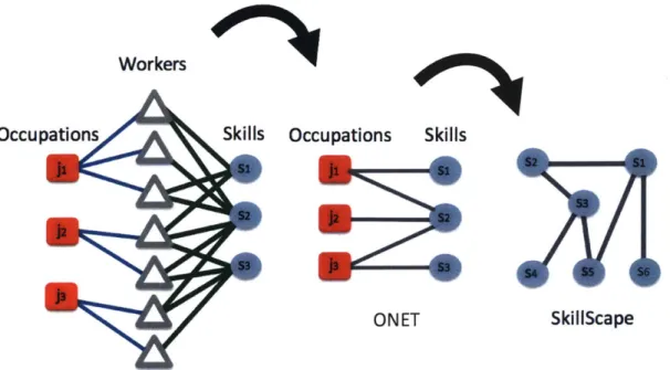
3-2 An occupation is identified through the skills of workers of that

occupa-tion. The bipartite network connecting occupations to required skills is a result of an underlying tripartite network containing workers as a conduit between occupations and skills. Relationships between skills

are determined from their co-occurring importance across occupations. 46

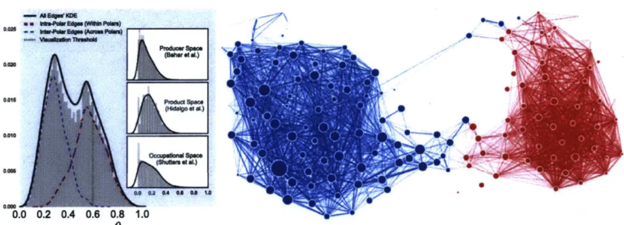
3-3 The distribution of all co-occurrence proximities between skills. Insets

represent counterpart networks from other related works of literature for comparison. Unlike previous applications of co-occurrence networks (insets), the SkillScape contains a bimodal distribution of pairwise skill

(15)

3-4 We identify two polars of skills by applying Louvain community de-tection to the complete SkillScape network (i.e. no minimum 0). We notice that this almost perfectly captures the right mode of the bi-modal distribution. That is, the links that are within one of the two clusters (intra-polar edges) mostly belong to the strong mode of the distribution, while the weak links within the weak mode almost exclu-sively belong to edges that are between clusters (i.e. inter-polar edges). The visual on the right only contains 0>.6 edges. The complete list of

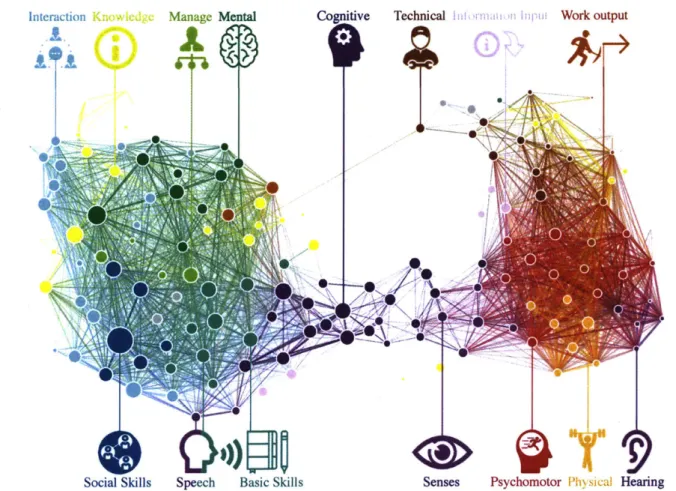
O*NET skills in each cluster is presented in the SI Appendix. .... 50 3-5 A filtered visual for the SkillScape. The SkillScape thresholded

ac-cording to a minimum skill similarity (i.e. 0 > 0.6) visibly reveals

two communities of complementary skills and respects expert-derived

O*NET categories (colors). Node sizes reflect the PageRank values,

while color indicates the O*NET categorization of the skill. . . . . 51

3-6 The SkillScape network respects experts' skill categorization. For each O*NET skill category, we measure the distribution of O's for pairs of

skills within a category (blue) and compare it to the distribution of O's for each edge connecting a skill within the category to a skill outside of the category (red). The complementarity for skills within a category is significantly stronger according to the KS statistic (title) than the

complementarity for skills across categories. . . . . 52

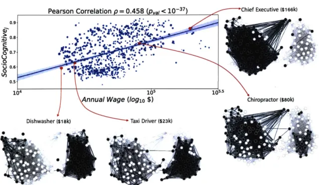
3-7 Four different occupations, showing how they drastically differ in SkillScapes.

Nodes of skills that an occupation requires (e(j, s) = 1) are maintained

(colored in black), while skills that the occupation does not require are ignored (colored in white). It is clear that a job such as (A) nuclear technician requires mostly sensory-physical skills, in contrast to (D) nuclear engineer, for example, which requires mostly SocioCognitive

sk ills. . . . .. 53

3-8 Occupations requiring more SocioCognitive skills tend to make higher

(16)

3-9 Performed out-of-sample testing for each model in table 3.1 through 1,000 trails of randomly selecting 75% of the occupations as a training

data set and measuring the root-mean squared error of the resulting model applied to the remaining 25% of occupations. We represent the resulting model performance as box plots. Medians are represented by

a red line, while the mean error is represented by the triangles. ... 55

3-10 The two identified clusters/polars of skills using Louvain community

detection from figure 3-4, superimposed on the SkillScape visual in figure 3-5. This demonstrates that our categorization of which skills belong to a "SocioCognitive" vs. "Sensory-Physical" cluster was agnos-tic to the skill labels/ categorization from experts, and was reached in

a purely data-driven bottom-up approach. . . . . 57

3-11 Reliance on SocioCognitive skills predicts increased annual wages. As a

baseline, we consider the relative importance of routine labor using rou-tine O*NET variables from [15]. In addition to cognitive skill fraction

(SocioCognitivej), we calculate the total skill content

(Ess

I(j, s))

of each occupation. Each educational variable represents the total em-ployment in that occupation whose highest educational degree is a high school diploma, bachelor's degree, etc. All variables were standardized before regression. Standard errors are reported in parentheses and asterisks indicate the statistical significance of coefficient approxima-tions. We perform out-of-sample testing for each model through 1,000 trails of randomly selecting 75% of the occupations as training data and measuring the root-mean squared error of the resulting model ap-plied to the remaining 25% of occupations. We represent the resulting model performance as box plots. Median error is represented by a red

(17)

3-12 The labor market network connecting jobs based on their coexistence

in cities, similar to the one presented by Shutters et al. Panel (A) The

job market network, with node colors representing the industry cluster

to which an occupation belongs, where red = Production Occupations;

blue = Education, Training, and Library Occupations; green =

Health-care Practitioners and Technical Occupations; cyan = Life, Physical, and Social Science Occupations; purple = Office and Administrative Support Occupations; and gray = all other clusters. (B) provides a closer examination of a subpart of the graph and a few examples of jobs that strongly "coexist" together. . . . . 61

3-13 Heat-map visualizations of the data. (A) represents the number of

employees for different occupations within the various cities. (B) rep-resents the relationships between occupations in the U.S. labor mar-ket and 161 skills "I(j, s)". (C) shows that by multiplying the BLS

city/occupation data set with the occupation/skill data set from O*NET, we obtain a matrix that relates all cities to every skill "I(c, s)". ... 62

3-14 The SkillScapes of different U.S. cities, showing an evolutionary path through different SkillScapes. Nodes of skills in which a city has

sig-nificant presence, i.e. e(c, s) = 1, are maintained (colored in black),

while other skills are ignored (colored in white). . . . . 63

3-15 Larger cities (i.e.. in population and number of workers in the labor

force) increasingly rely on SocioCognitive skills, leading to economic well-being (e.g. higher median household income and GDP). Example cities are projected onto the SkillScape using black nodes for effectively

used skills. . . . . 64

4-1 Frey and Osborne's [54] automation probabilities superimposed onto

(18)

4-2 (A) Relationship between the predicted impact of automation on cities

and the cities' SocioCognitivec metric. (B) Relationship between the

predicted probability of automation for occupations and their SocioCognitivej

fraction . . . . 70

4-3 Skill proximity predicts worker transitions between occupations, skill redefinition of occupations, and skill acquisition in cities. (A) An example demonstrating SkillScape proximity (i.e. proximity(j, s)) as a proxy for the connections between effectively used skills and other skills. (B) Skills with high proximity to the effectively used skills of an urban labor market in 2010 are more likely to be effectively used

by that work force in 2015. (C) Skills with high proximity to the effectively used skills of an occupation in 2010 are more likely to be effectively used by that occupation in 2015. (D) The effectively used skills in a worker's occupation in 2015 are more likely to be effectively used in the worker's next occupation in 2016. We provide bar plots including 95% confidence intervals for these probabilities in SI figure

8-7, and we consider an alternative area under the receiver operating

characteristic curve (AUROC) analysis in SI figure 8-14. . . . . 74

4-4 The polarized skill network constrains worker mobility. Binning by the SocioCognitivej of the worker's occupation in 2014 reveals the (A) expected SocioCognitive change and (B) the expected magnitude of

SocioCognitive change when workers change occupations. Random oc-cupation selection is considered as a null model (gray). Standard error bars are provided, but are small. Actual occupation transitions are pro-vided as examples in (A). (C) The national distribution of employment

by SocioCognitivej with the distribution of individual occupations as

(19)

4-5 The connectivity and embeddedness for each skill category (by aver-aging the zscores for the PageRanks that each skill possesses in each skill category). The measure corresponds to worker mobility because skill proximity is indicative of skill acquisition. This highlights the im-portance of social skills for labor mobility. For a detailed result of all

skills, see fig.8-2. . . . . 77

4-6 The growth rate exponents for the two skill clusters (SocioCognitive vs. sensory-physical). This demonstrates that the occupations that have SocioCognitive skills grow superlinearly with city size and therefore, the presence of such skills in cities also grows superlinearly with city

size . . . . . 78

5-1 Figure recreated from [84]. Gumbel probability distribution of

im-perfect transmission, based on Henrich [61]. This demonstrates how transmission and learning, which are facilitated by social ties, are prone to error (i.e. the distribution is attempting to mimic the transmitted skill value represented by the dash line). Some of those "distortions" are beneficial and are actually innovations that increase the value of the "skill". Those innovations and advancements are facilitated by the

increased connectivity of social ties (in quantity or diversity). . . . . . 83

5-2 Figure recreated from [6], where they studied communication

effective-ness. This plot demonstrates the results of their empirical analysis and findings where they highlight the fact that optimal case is a balance

between heterophily and lack thereof (i.e. homophily). . . . . 85

(20)

5-4 This figure demonstrates the results of using the feature vectors pro-duced by the proposed model vs DeepWalk for predicting the occupa-tion and gender of individuals in the TMDB network. Even though our model was tested on a variety of data sets, this results highlights both homophily and heterophily at the same time. Since our pro-posed model, which considers both drivers, outperforms DeepWalk in predicting occupations (reasonably assumed to be more driven by het-erophily), while it underperforms in Gender prediction which is as-sumed to be more driven by homophily (which DeepWalk is purely

focused on). . . . . 88

6-1 The strength of different indicators for the prediction of anomalous

behavior. Results demonstrate that social ties are better predictors

than "tweet" or profile contents. . . . . 94

6-2 The three messages shown to the three different groups, Control, Self

Information Leakage, and Social Information Leakage Group,

respec-tively. . . . . 95

6-3 The decision analysis results, which show the differences between each

group in terms of users' response to the SIL message, in addition to the media time taken to make the decision. The results show that the

third group behaves differently than the other two groups. . . . . 97

6-4 Snapshot of the social network of the Friends and Family data set. We can see many features, such as stronger and more bidirectional ties within cliques than across the clusters that were identified through the clustering algorithm (which is stronger than random, and visually

(21)

6-5 Probability distribution for 10,000 two-dimensional points from three

different one-dimensional laplacian noise generations at different loca-tions

(E

= .3 (blue), E = .4 (green), & E = .5 (red)). The middle inset

plot is a scatter plot of the generated noise points, while the left plot represents many probability density functions for the noise points in

two dimensions , and the right plot is a two-dimensional heat-map for

the noise points. . . . . 101

6-6 Architecture for the behavioral privacy algorithm. . . . . 103

6-7 Approach for comparing utilities of the state-of-the-art vs. the

pro-posed behavioral privacy method. . . . . 104

6-8 The state-of-the-art method (red) vs. the behavioral privacy variant

(blue), using different privacy parameters (x-axis) and then applying a linear SVM on the resulting distorted data sets. We show the re-sulting utility measures (AUROC values) on the y-axis. Inset plots represent the kernel density estimator (KDE) and cumulative distri-bution function (CDF) for the y-axis when aggregating over all of the

x-axis. . . . . 105

6-9 Aggregated resulting p-values for all individuals in the data set using

the various machine learning algorithms demonstrated. Each machine learning method is the aggregation of the various kinds of results (e.g.

Call/Bluetooth -> Stress/Happiness) for all users. The 344 data sets

represent around 86 individuals, each having four possible

(22)

7-1 A summary for the flow of the thesis, starting from the initial

chap-ters that transformed matrices of individuals' job features to construct the skill network, which demonstrated the importance of the social dimension in the labor force (for both economic well-being and labor mobility). Then, using a city's social network, later chapters employed a mechanistic model to capture the value of social ties for social ex-change by reconstructing the individuals' features embedded in the

social network. . . . . 110

7-2 Cities with various sizes are at different stages of evolution for their skill

portfolio. That is, smaller cities, on the left, mostly possess Sensory-Physical skills, while larger cities, on the right, possess mostly

So-cioCognitive skills. . . . . 111

7-3 (A) An example current status of acquired skills in the SkillScape.

This could be an individual, occupation, or city. (B) demonstrates the

weighing of costs and benefits for various skill acquisitions. . . . . 111

8-1 Transforming raw O*NET data with RCA. The first plot is the raw

skill matrix, I(j, s), the middle plot is the RCA occupation-skill matrix, rca(j, s), and the final plot is the thresholded RCA job-skill matrix, e(j, s), for 2014. Here, e(j, s) = 1 if and only if rca(j, s) >

1. Occupations (y-axis) are ordered by the sum of threshold RCA

skill values, and skills (x-axis) are ordered by the correlation of their

thresholded RCA values across occupations to the occupational sums. 113

8-2 Full list of skills for figure 4-5 in the main text. PageRank scores for

every individual Skill (node in the network). That is, the connectivity

& embeddedness of each skill. Color represents skill category. . . . . 115

(23)

8-4 Instead of PageRanks in figure 4-5 (which is an n-th order calculation), this is the first order calculation for comparison. This figure demon-strates complementarity scores for every skill category. That is, the average Z-score of each categories' node strengths (sum of it's edges, or "complementarity weights" 6). Color represents skill category. We

can see Social Skills still achieve the highest score. . . . . 117

8-5 Complementarity scores for every individual Skill (node in the

net-work). That is, the Z-score of each node's strength (sum of it's edges,

or "complementarity weights" 0). Color represents skill category. . . 118

8-6 Continuing Node Strengths of the SkillScape Skills. . . . . 119

8-7 Instead of the interpolated plots in the main text (figure 4-3), here we

provide bar plots with the associated error bars. . . . . 120

8-8 Out of sample testing of model performance from Table 8.2. For each

model, 1,000 trials are run where 75% of the data is randomly selected as training data and the remaining 25% of data is used as validation. The distribution root-mean-square errors for each model is reported. Medians are represented by a red line, while the mean error is

repre-sented by the green square. . . . . 122

8-9 Out of sample testing of model performance from Table 8.3. For each

repre-sented by the green square. . . . . 123

(24)

repre-sented by the green square. . . . . 126

8-12 A cartoon example of AUROC calculation. . . . . 127 8-13 The top figures represent the fraction of instances (for cities or

occu-pations) that have a change (i.e. Acquiredf1 2) with the x and y axis

representing the respective A1 and A₂values. While the dotted boxes in

each of the top figures represent the zoomed area that the AUROC val-ues will be studied in the bottom figures. The bottom figures represent comparison of AUROC distribution for all of the various cities of occu-pations. That is, for each A, and A2 value, there are many instances of

cities or occupations that have such a change, and we study the AU-ROC results for predicting such jumps using the different indicators

(raw onet, RCA, or SkillScape's proximity metric). . . . . 128

8-14 The varying averages of AUROC achieved by combining the differ-ent variables with varying degrees (two network based, and one raw data based), creating this Dirichlet triangle. SkillScape is a network

features, while I & LQ are none network features. . . . . 129

8-15 The skill requirements of an occupation indicate the education

re-quired. In each panel, we plot the SkillScape network thresholding edges with 6 > 0.6. Nodes (or skills) are colored according to the Pearson correlation between onet(j, s) and the proportion of workers of each occupation with a given degree (title). . . . 130

8-16 The correlation between social status and degree distribution in the

Andorra dataset. .. ... ... .. . ... . .. . . . .. 131

8-17 The correlation between human capital and social capital in TMDB

(25)

List of Tables

3.1 We consider the SocioCognitive skill fraction (SocioCognitivej) and

the total embeddedness (EZcs I(j, s)) of each occupation in addition

to educational variables in linear regression models. Each educational variable represents total employment in that occupation whose highest educational degree is a high school diploma, bachelor's degree, etc. All variables were standardized before regression. Models for occupational wages are improved and less susceptible to over-fitting when accounting for the SocioCognitive skill fraction of occupations, as can also be seen

in fig.3-9. . . . . 55

8.1 Descriptions of each occupation type indicator variable used in

regres-sion models. For each occupation, the indicator variable is 1 if and

only if the occupation SOC code belongs to that occupation category.

Each occupation belongs to exactly one occupation category. . . . . 121

8.2 Linear regression using standardized SocioCognitivej for each

occupa-tion and occupaoccupa-tion type indicator variables. . . . . 121

8.3 Linear regression using SocioCognitivej and employment in each

oc-cupation with a bachelor's degree (denoted B.D. Employment) and without a bachelor's degree (denoted No B.D. Employment). Each variable has been standardized. Employment by level of education for

(26)

8.4 Linear regression using standardized SocioCognitivec for each city and employment in that city of each occupation type. All variables have

been standardized. . . . . 124

8.5 Linear regression using SocioCognitivec and education variables.

Ed-ucation variables represent the employment in each city by highest

(27)

Chapter 1 Introduction

1.1 Introduction

By 2050, it is expected that 66% of the world population will be living in cities [85].

The urban growth explosion in recent decades has raised many questions concerning the evolutionary advantages of urbanism, with several theories delving into the multi-tude of benefits of such efficient systems. This thesis focuses on one important aspect of cities: their social dimension, and in particular, the social aspect of their complex socioeconomic fabric (e.g. labor markets and social networks). Economic inequality is one of the greatest challenges facing society today, in tandem with the eminent impact of automation, which can exacerbate this issue. The social dimension plays a significant role in both, with many hypothesizing that social skills will be the last bastion of differentiation between humans and machines, and thus, jobs will become mostly dominated by social skills.

Using data-driven tools from network science, machine learning, and computa-tional science, the first question I aim to answer is the following: what role do social skills play in today's labor markets on both a micro and macro scale (e.g. individuals and cities)? Second, how could the effects of automation lead to various labor dy-namics, and what role would social skills play in combating those effects? Specifically, what are social skills' relation to career mobility? Which would inform strategies to mitigate the negative effects of automation and off-shoring on employment. Third,

(28)

given the importance of the social dimension in cities, what theoretical model can explain such results, and what are its consequences? Finally, given the vulnerabili-ties for invading individuals' privacy, as demonstrated in previous chapters, how does highlighting those results affect people's interest in privacy preservation, and what are some possible solutions to combat this issue?

1.2 Thesis Outline

I begin by demonstrating a network science method applied more than once in my thesis. I utilize causal inference to illustrate its value in one instance, in addition to comparing its variants. In the next chapter, I apply that method in one case study on the occupations of individuals. The aim is to highlight the value of social skills in occupations, their relation to education, and annual wages. Subsequently, I extend the approach using a few adaptations to fit the larger scale of labor markets, which demonstrates the importance of social skills for cities and their economic well-being. The following chapter then deals with the critical issue of the negative impact of automation on cities and individuals. The chapter discusses how the approaches and structures proposed in the previous chapter can be utilized to combat those negative effects using individually optimized retraining and educating programs. In addition, the chapter also presents a website tool created for such an objective. Next, the following chapter delves into a theoretical explanation of the previous results and observations and proposes a computational model for social tie formation that would highlight the benefit for social exchange and trade. This chapter then applies the proposed model on a few small- and large-scale empirical datasets to test the validity of the approach and demonstrate some of its capabilities. Finally, the last chapter addresses some of the privacy concerns that the previous chapters might raise. It first presents an experiment conducted to examine whether people would in fact have increased concerns, after which it proposes an approach to tackle the issue by introducing the concept of decoupling privacy from utility, followed by proposing an algorithm.

(29)

Chapter 2 Methods

This chapter presents one of the methods used multiple times in my thesis, and ap-plies causal inference to show its value in one instance. This method is the "product space", which has been applied to countries and products, in contrast to our applica-tion in this thesis being labor markets. The product space provided a new vantage point for understanding the ecosystem of product creation through exports and its possible future changes, which is key when evaluating countries' economic strength. The literature [63, 62, 59, 103, 41, 42] has shown many methods of using network science to evaluate the underlaying structure of product creation, in addition to pro-viding the ability to predict future product exports [32]. The aim of this section is to analyze these methods, evaluate them, and compare their power for predicting economic evolutions. The goal is to adapt these methods for our own use in later sections.

2.1 Introduction

In "The Product Space Conditions the Development of Nations" [62], Hidalgo et al. took a unique network science approach (fig.2-1) to analyze production ability; then, in "The Building Blocks of Economic Complexity" [63] they used their outputs to evaluate a country's level of economic complexity and predict its future economic growth. Furthermore, Haussman et al. [59] showed how network science could be

(30)

Figure 2-1: Illustration of the product space connecting 775 products based on their

proximity matrix. The color of the node represents the product classification. This

is my replication [63, 59, 62] based on 2013 data.

used to evaluate a country's competitiveness in products and therefore the knowledge it possesses to engineer those products. One of the most critical outputs of Hidalgo and Hausmann's work was providing an original approach to measure the economic

complexities of countries based on a network view of international trade data (i.e. the

product space) using the method of reflection (MR). While this method proved to be useful for their analysis and the results that followed [63, 59, 62], later publications, first Tacchella et al.'s "A New Metrics for Countries' Fitness" [103] and later Cristelli et al.'s work [41, 421, have argued for other methods, converging on a method named

"fitness", which has a different mathematical formulation than complexity. They

argued for their metric's stability, and stated that it assimilated more of the theory.

Though extensive work has been published on the shortcomings of one method vs.

the other, and though quantitative comparisons have been made [41, 42], no causal inference comparison between the methods has been published, either individually or pair wise.

(31)

2.2 Methods and Results

The main resource used in this work is the World Bank, which reports data about the world development indicators (WDI) for most countries. However, for data on per capita GDP at Purchasing Power Parity (PPP), the International Monetary Fund (IMF) is used. The main years used in the analysis are 1985, 1990, 1995, 2000, and

2005.

First, we discuss and analyze the parts of the methods on which both approaches agree, before discussing the areas where they diverge. To analyze the bipartite net-work of countries and products, we first define whether or not we consider a country to be connected to a product:

_____ EZdXCIP

I if>

MCP=

fi

if EP "' (2.1)

0 otherwise

Where "c" represents a country and "p" represents some product. Xc, is the value of exports of product p from country c, while Mc uses Xcp to decide whether or not country c has a comparative advantage in product p. If the fraction of product p exports out of country c is higher than the fraction of product p in the global export trade of the world, then country c indeed exports product p with a comparative advantage, otherwise it is not considered to be an exporter of p. For example, if oil represents 1% fraction of the world export trade, then a country needs more than 1% of its exports to be oil for it to be significant enough to be considered as an exporter of oil with a comparative advantage.

At this point, each method diverges in how it evaluates each node (country or product) in the network. In building the economic complexity index, Hidalgo et al. [62] characterized countries and products by introducing a set of variables that capture the structure of the network defined by Mc. Their methodology consists of iteratively calculating the average value of the previous-iteration properties of a node's neighbors and is defined as the set of observables:

(32)

k,n = I Mckp,n1 (2.2)

k = k, Mckcn_1 (2.3)

Initially, kc,O and kp,O represent the number of products with significant prominence out of country c, and the number of countries that export product p with significant prominence, respectively. n > 0 indicates the number of iterations of refinement that

the metric has gone through. Therefore, kc,n converges to the country complexity

index CCI, see fig.2-2, and kp, converges to the product complexity index PCI for

large n values.

These network representations of the data have shown great success in capturing information about a country's level of "knowhow and knowledge" [59], demonstrated

by predicting new exports of countries and correlating to GDP growth, even when

controlling for various covariates [62]. It is important to note that instead of defining economic growth as the difference of logs between two years [62], we use a more accepted definition of it as the annualized growth rate:

Annualized GDP Growth(t, t' = t + At) = [(Dt )1/At - 1] * 100

The regressions' coefficient values and their significance estimates using this metric for economic growth are somewhat different than the ones reported in Hidalgo et al.'s original paper. This is to be expected given the change to the way economic growth is calculated. However, their hypothesis and final conclusions still hold.

Even though the previously discussed method has shown tremendous results, some in the literature have claimed that there are theoretical issues with it [103], ranging from assimilation of the theory [41], to instability of the method's iteration values (see first plot in fig.2-2) [42]. To tackle these issues, a new method was developed in

(33)

I,n=

Ep Mckp,n I

kc,n = Ic,n/ < Ikc,n >

Ip,n/ <

k,n

>

This new version of the method (referred to as "fitness") is very similar to the previous method (i.e. "complexity"). This can be seen from the work of Albeaik et al., which demonstrates that both methods have the same raw equation form with

differing parameters (i.e. (a, ,, , e, 6) which can only take the values of (1,0,-i))

[4]: kc ₌ ( E, ~ _(EPMepkp'n)^ MCP)E (k ZMcpkfn)' p , + ( ZM =) 6c

(EZC

MCP) 0 (2.4) (2.5)

where (a,

/3,

7, 6, E, 0) are parameters that produce a family of metrics (36 =729),

with (1, 1, 1, 1, 1, 1) producing complexity and (1, -1, 1, -1, 0, 0) producing fitness.

kp,n =

(34)

(A) Complexity (All Iteration Values)

0 1 , , 1

5 10 15

(C) Complexity

(Z-scored Even Iteration Values)

a)

E

U

(B)

Complexity (Even Iteration Values)

E U-8~ a0 5 10 15 (D) Fitness

(All Iteration Values)

1iz

10 15 10 15

Iteration Number Iteration Number

Figure 2-2: Complexity and Fitness methods' convergence plots. Plot (A) shows all iterations of the complexity method, while plot (B) only shows the even iterations. Plot (C) however, is the z-score for each even iteration of complexity, making it more closely resemble fitness. Finally, plot (D) shows all Iterations of the fitness method.

First, it should be noted that there are significant impacts (as can be seen in the last plot of fig.2-2) for normalizing in each iteration and taking the reciprocal of the sum of the reciprocals, which is done in the fitness approach. It is clear that the newer method of fitness is stable even when viewing the raw evaluations (in contrast to complexity's raw iterations, fig.2-2). Second, fitness converges to a steady state,

E -0 U

S-cm

(35)

but it does not converge to the same value as complexity does (with the variance becoming smaller and smaller in magnitude with more iterations).

2.3 Quantitative Comparison

First, in order to quantitatively compare the two methods, we can run the same regressions previously done [62] after modifying how GDP growth was calculated, and we can then compare the regression results of the two methods. For example, regressing the two methods over the GDP per capita values for different years and

comparing resulting Adjusted R2 _{produces an interesting result (see fig.2-3). Namely,}

Figure 2-3 shows the effects of the instability in the complexity method and how well it fits the dependent variable in different iterations. The results also show that complexity produces a better fit than fitness does, even though fitness is more stable and reaches a steady state faster. It should be noted that the superiority of one

method over the other in these R2 results is not indicative of much, since there are

(36)

Co

6 '~ --- 2005

--- ₂₀₀₀ ₉

-- 1995 A.

--- 1990

-e even iterations of Complexity

' odd iterations of Complexity

"D.

*a

Seven iterations of Fitness

Sodd iterations of Fitness

= . j. II '

0 5 10 15 20

Complexity I Fitness

Figure 2-3: Adjusted R2 values (y-axis) from regressing GDP for various years over the successive iterations (x-axis) of the two different metrics (complexity and fitness).

However, the hypothesis presented in the original literature hints towards a causal link. Hence, we further examine the relationship between GDP and the two different methods. To this end, we use GDP growth as our dependent variable, as the hypoth-esis presented in the literature indicates such a link. In addition, we add a few control variables to ensure that no meaningful and reasonable confounders that we should control for are left unused. The first of these control variables is the original GDP value at the initial point of time, to control for the size of the economy. The second is population size, as this could explain economic growth. The last control variable is the total enrollment in tertiary education, expressed as a percentage of the total

(37)

population, as education could also explain economic growth. As for the treatment, we use a binarized value for the two metrics (larger than the average or less than the

average):

Annualized GDP Growth(t, t') ~ treat + GDP(t) + Pop(t) + Edu(t) + C (2.6)

where GDP represents the log of a country's PPP GDP per capita, Pop is the log of the country's population, and Edu is the percentage of enrollment in that country's tertiary education. Moreover, t and t' they represent the year under study, with

t' = _{t + At, and treat is the treatment variable(i.e. binarized complexity or fitness).}

Converting the treatment into a binary variable has some significant implications for what relates back to the raw metric, but one can assume that if the binary version shows a causal relationship, then that should generalize to the raw variable. Hence, the only result we hope to obtain this experiment is whether or not either or both treatments are indicative of economic growth; we do not assume that we can gain a good measurement of the magnitude of that relationship. Thresholding the treatment metric significantly hinders our ability to test its causality links, but if we still find a causal link after thresholding, that evidence will transfer to the continuous version as well. Otherwise (in cases where no statistical evidence is found), nothing can be stated about any causal link with regard to the continuous version. We do this for both treat = binary(Complexity), and treat = binary(Fitness). However, before running our regression, we use matching to approximate (simulate) a controlled experiment and reduce the imbalance in the covariates as much as possible. The method we use for matching is the coarsened exact matching (CEM) method for the cases of two and all three covariates (see fig.2-4).

(38)

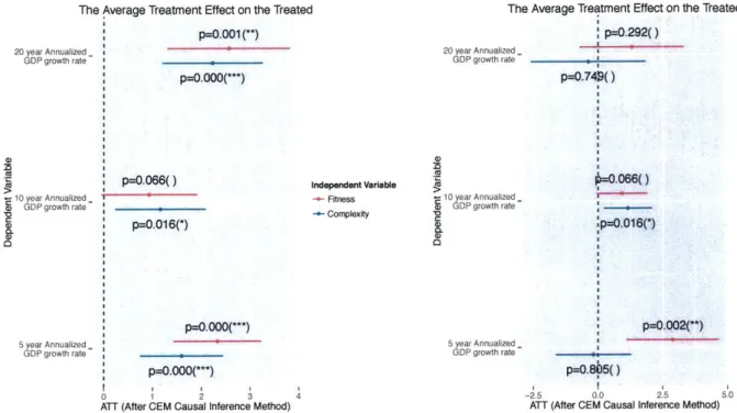
The Average Treatment Effect on the Treated

p=0.001(**)

20 year Annualized

GDP growth ratep

10 year Annualized-(UGOP growth rate

W CL a) 4) aU p=0.066() p=0.016(*) p=O.000(***) 5 year Annualized GDP growth rate-P-=0.000<---) 0 1 2 3

ATT (After CEM Causal Inference Method)

Independent Variable

+ Fitness

- Complexity

The Average Treatment Effect on the Treated

p=0.292() 20 year Annualized-GDP growth rate p=0.740() a) 10 year

Annualized_-aGDP growth rate

CL 0=0.066() :p=0.016(*) p=0.002(**) 5 year Annualized-GDP growth rate p=O.85() -2.5 0.0 2.5

ATT (After CEM Causal Inference Method)

4

Independent Variable

+ Fitness + Complexity

5.0

Figure 2-4: The average treatment effect for the treated (the ATT statistical method) on GDP growth (for both the complexity and fitness treatments), after matching and controlling for covariates. The left results are without education, while the results on the right add the covariate of education. It should be noted that the fact that the right plot demonstrates non-significant results is mostly because the coarsened exact matching removed too many data points, see fig.2-6.

After matching and controlling for covariates, we see that both complexity and fitness mostly have a large, statistically significant effect when regressing over eco-nomic growth (5 years and 20 years, but not 10 years). This does not mean that there is an issue with the 10-year growth rates, but that the problem is the lack of data points after matching for that time period (see fig.2-5 and fig.2-6). Figure 2-4 demonstrates a causal relationship between both complexity and fitness and GDP growth when controlling for two covariates.

Although coarsened exact matching is powerful in enhancing our ability to control for confounders, it omitted a significant amount of the limited data we had (right figure in fig.2-6). Fortunately, we still see that there is a significant sign for a causal link, and therefore conclude that complexity (and in a similar result, its variation fitness) both capture a dimension that has a causal impact on economic growth for countries (independent of the population and economic size), with no method having

(U

a)

(39)

3.0 3.5 log10 GDPpc (PPP) 4.0 4.5 9 -0-0 T. S * 05. * S S 0 * *

Figure 2-5: The coarsened exact matching scatter plot visual for the two-variate matching, to demonstrate which data points were kept (matched) vs. dropped (un-matched). We see a significant number of remaining data points for statistical

anal-ysis.

Max

-Min

GDP Population Years of education

Max

-Min

-GDP Population Years of education

Figure 2-6: This figure demonstrates the data points kept by the coarsened exact matching method, with the left figure being identical to fig. 2-5, and the right plot representing the three-variable variant of the matching. Note the limited number of remaining (matched) data points in the three-variable matching.

a

0 .2

Type

* not Matched & not Treated not Matched & Treated Matched & not Treated * Matched & Treated

2.5

- Not Matched & Not Treated - Matched & Not Treated

- Not Matched & Treated - Matched & Treated

- Not Matched & Not Treated! - Matched & Not 7wated

(40)

a significant advantage over the other.

2.4 Conclusion

These preliminary analyses indicate that further investigation might prove fruitful, such as incorporating causal inference analysis to study what relationships these met-rics have with other economic factors (unemployment, income inequality, resistance to shocks). In addition, it could be interesting to conduct a deeper analysis of the methodologies applied and the parameter choices that were made, and whether other directions might be more appropriate. However, the results generally indicate that there is good reason to adopt these methods for our purposes in this thesis of studying the labor market dynamics of individuals/ cities and their skills.

(41)

Chapter 3 The Importance of Social Skills in

Labor Markets

This chapter discusses the role of social skills in today's labor markets on both a micro and macro scale (e.g. individuals and cities). Specifically, the chapter introduces a novel approach of constructing a complementarity network for all of the skills in the labor market. Thus allowing us to unpack the polarization of workplace skills, which has been deemed to be the cause for the hallowing of the middle class, and then we investigate the value of social skills for occupations' salaries and labor markets' (i.e. cities') economic well-being.1

3.1 Introduction

Economic inequality is on the rise, making it one of the central challenges facing policy-makers today [67, 5, 39]. In recent decades, the middle class has shrunk in the vast majority of U.S. metropolitan areas [34]. For example, consider that absolute income mobility-the fraction of children who earn more than their parents-has fallen dramatically in the U.S. from 90% for children born in 1940 to 50% for children born in 1980 [36]. Some have declared that the diminishing opportunity for prosperity and

'This work is to be published in "Ahmad Alabdulkareem, Morgan Frank, Lijun Sun, Bedoor Alshebli, Cesar Hidalgo, and Iyad Rahwan. Unpacking the polarization of workplace skills. Science Advances, 2018."

(42)

success marks the fading of the "American dream" [93, 65], an ideal that is intimately associated with the U.S.'s national identity and ethos. This highlights the growing need to characterize low- and high-wage occupations, and to identify the constraints on career mobility between the two.

In contemporary political debate, one of the main culprits behind economic in-equality is the lack of "good jobs". Both nationally and in a majority of U.S.

metropoli-tan areas [34], _{economists have identified occupational polarization: an increasing}

proportion of high- and low-wage employment, accompanied by a relative decrease in employment share in middle-wage occupations [13, 14, 1]. The result is a "hollowing" of the middle class. Mechanisms driving this trend include the off-shoring of work [48], which has triggered recent shifts in international trade policy. Another mecha-nism is the automation of routine work, which has sparked major concerns about the impact of automation on the future of work [75, 12, 24].

However, while mechanisms like off-shoring and automation ultimately impact people's jobs, they do not typically operate at the level of occupations. Rather, they alter the demand for specific workplace skills, tasks, knowledge, and abilities (hereafter, "skills"). Thus, if individual workers, or even entire cities, are unable to adapt their own skills appropriately, their ability to compete in the national and global labor market may be diminished.

Despite the important role of skills in occupational polarization, existing studies have explained the hollowing of the middle class in terms of annual wages [11] and broad, subjectively defined occupational categories, such as "cognitive" versus "phys-ical", or "routine" versus "non-routine" [13]. For example, suppose we use wage as a proxy for skill (that is, high-wage occupations are considered high-skilled occupa-tions, etc). Then, if we find that growth in employment in middle-wage occupations is slower than growth in low-wage and high-wage occupations, we may conclude that demand for high-skills and low-skills are driving economic inequality. However, this coarse-grained distinction may miss important relationships between skills that im-pact how workers adapt. This motivates the set of questions we wish to explore in this chapter:

(43)

Q.

Can we recover occupational polarization, at the finer-grained level of underlying skills, using an objective (unsupervised) data-driven clustering? How many distinct clusters, if any, does this skill structure contain? And does the skill structure exhibit smooth or abrupt transition between skill clusters?

To answer these questions, we apply data-driven methods to map skill complementar-ity as a network. We find that workers leverage skill complementarcomplementar-ity between their

existing skills to make career changes

[31].

Similarly, cities leverage complementarity

between industries to optimize productivity and increase their competitiveness in a

global economy [91, 92, 87, 86]. We use techniques from network science to identify

distinct clusters of skills, and we find that the structure of skill complementarity ex-plains many stylized observations about occupational polarization and the hollowing of the middle class.

3.2 Data Sets

The first data source for this chapter is the Occupational Information Network (O*NET): a program by the U.S. Department of Labor which annually produces a publicly avail-able database detailing the importance of 161 workplace skills, knowledge, and abili-ties for the completion of each of the 672 occupations recognized under the Standard Occupational Classification (SOC) System, see figure 3-1.A.

This allows us to understand not only the decomposition of any given occupation, but also its relationship to all other occupations. The O*NET database is updated regularly, allowing for annual snapshots of the relationships between occupations and skills through continual survey of workers from each occupation. We use annual

O*NET data from the years 2010 through 2015. We denote the importance of skill

s E S to occupation

j

E J using I(j, s) E [0, 1], where I(j, s) = 1 indicates that s is

essential to

j,

while I(j, s) = 0 indicates that workers of occupation

j

does not need

Analyzing cities' complex socioeconomic networks using computational science and machine learning

Analyzing Cities' Complex Socioeconomic Networks

Using Computational Science and Machine Learning

Ahmad Alabdulkareem

@

Signature redacted

Signature redacted

Signature redacted...

//

Signature redacted

Signature redacted

JUL 26 2018

Analyzing Cities' Complex Socioeconomic Networks Using

Computational Science and Machine Learning

by

Ahmad Alabdulkareem

Doctor of Philosophy in Computational Science & Engineering

Abstract

Acknowledgments

Contents

List of Figures

(Ess

(E

List of Tables

Chapter 1

Introduction

1.1

Introduction

1.2

Thesis Outline

Chapter 2

Methods

2.1

Introduction

2.2

Methods and Results

fi

I,n=

k,n

(EZC

/3,

2.3

Quantitative Comparison

2.4

Conclusion

Chapter 3

The Importance of Social Skills in

Labor Markets

3.1

Introduction

Q.

[31].

3.2

Data Sets

j

j,

j