Publisher’s version / Version de l'éditeur:
Vous avez des questions? Nous pouvons vous aider. Pour communiquer directement avec un auteur, consultez la première page de la revue dans laquelle son article a été publié afin de trouver ses coordonnées. Si vous n’arrivez pas à les repérer, communiquez avec nous à [email protected].
Questions? Contact the NRC Publications Archive team at
[email protected]. If you wish to email the authors directly, please see the first page of the publication for their contact information.
https://publications-cnrc.canada.ca/fra/droits
L’accès à ce site Web et l’utilisation de son contenu sont assujettis aux conditions présentées dans le site LISEZ CES CONDITIONS ATTENTIVEMENT AVANT D’UTILISER CE SITE WEB.
Minerals Engineering, 134, pp. 281-290, 2019-02-13
READ THESE TERMS AND CONDITIONS CAREFULLY BEFORE USING THIS WEBSITE.
https://nrc-publications.canada.ca/eng/copyright
NRC Publications Archive Record / Notice des Archives des publications du CNRC :
https://nrc-publications.canada.ca/eng/view/object/?id=6e50762a-a01d-49f8-82bd-6eb0ee7cf8b5 https://publications-cnrc.canada.ca/fra/voir/objet/?id=6e50762a-a01d-49f8-82bd-6eb0ee7cf8b5
NRC Publications Archive
Archives des publications du CNRC
This publication could be one of several versions: author’s original, accepted manuscript or the publisher’s version. / La version de cette publication peut être l’une des suivantes : la version prépublication de l’auteur, la version acceptée du manuscrit ou la version de l’éditeur.
For the publisher’s version, please access the DOI link below./ Pour consulter la version de l’éditeur, utilisez le lien DOI ci-dessous.
https://doi.org/10.1016/j.mineng.2019.02.025
Access and use of this website and the material on it are subject to the Terms and Conditions set forth at
Multiphase mineral identification and quantification by laser-induced breakdown spectroscopy
El haddad, Josette; De Lima Filho, Elton Soares; Vanier, Francis; Harhira, Aïssa; Padioleau, Christian; Sabsabi, Mohamad; Wilkie, Greg; Blouin, Alain
1
Multiphase mineral identification and quantification by
laser-induced breakdown spectroscopy
Josette El Haddada*, Elton Soares de Lima Filhoa,1, Francis Vaniera,1, Aïssa Harhiraa,1, Christian Padioleaua, Mohamad Sabsabia, Greg Wilkieb, and Alain Blouina
a
Energy, Mining and Environment Research Centre, National Research Council Canada, 75 de Mortagne, Boucherville, J4B 6Y4, Canada
b
CRC-ORE, 1, Technology Court, Pinjarra Hills, QLD 4069, Australia
1
These authors contributed equally to this work.
*
Corresponding author:
E-mail address: [email protected]
Abstract
Quantitative mineral analysis (QMA) performed using energy-dispersive x-ray spectrometry and scanning electron microscopes (EDS-SEM) provide reliable information on the mineral abundance and texture of prepared rocks. This information helps in the optimization of the mining and milling processes, and to define the value of a deposit. Real-time analysis of coarse rock streams would greatly enhance the decision-making processes driving the mining operation efficiency; however electron-microscope-based instruments are not yet adaptable for in-field measurements. Laser-induced breakdown spectroscopy (LIBS) has been used for elemental analysis in many environments but has not been employed for true mineral quantification and identification. This work presents a new method for mineral identification and quantification
2
using LIBS, which could be scalable to perform automated mineralogy measurement in coarse rock streams. A set of rock tiles from mining operations in Australia had QMA performed using an EDS-SEM instrument and the resulting data were used to guide and validate the results obtained by LIBS. The use of a multivariate curve resolution – alternating least square (MCR-ALS) method applied to the LIBS data allowed the identification, quantification and imaging of minerals on rock tiles, even in the presence of mixed mineral phases within the laser spot area. Mineral abundance and imaging are obtained with success for the mineral phases selected in the present work, which includes bornite, chalcopyrite, pyrite, molybdenite, quartz, chlorite, K-feldspar, albite, fluorite and calcite. The method presented a mineral quantification root mean square error below 10 % for the main minerals. In addition, mineral quantification by point-counting using single laser shots per LIBS measurement is demonstrated, achieving absolute errors below 3.5 % for major minerals and below 1 % for minor minerals.
Keywords: Mineral phases identification; LIBS; MCR-ALS; quantitative mineral analysis.
1
Introduction
Laser-induced breakdown spectroscopy (LIBS) is a form of atomic emission spectroscopy where the light from a plasma plume created on the surface of the material is analyzed. It has the advantage of analyzing the material without contact, making it suitable for in-field and real-time analysis of any type of material, whether in the solid, liquid, slurry or gas phases (Hahn and Omenetto, 2010, 2012). Due to its flexibility and robustness, LIBS has been demonstrated in various environments, ranging from the wet, high-pressure ocean bottom (Angel et al., 2016; Yelameli et al., 2016) to the hash surface of Mars (Wiens et al., 2013). LIBS is of great interest in several industrial sectors (Noll, 2012), where there is a need for fast elemental analysis that cannot be addressed by conventional analytical methods. Also, LIBS is a good candidate for several applications in the mining industry (Rifai et al., 2017). For instance, LIBS has been successfully used by several research groups to perform elemental analysis and imaging in geological materials (Harhira et al., 2018; Harmon et al., 2017a; Harmon et al., 2009; Moncayo et al., 2018; Qiao et al., 2015; Washburn, 2015).
The mining industry is interested in knowing the mineral composition of rocks, rather than just their elemental composition. By knowing the mineral phases present in rock samples, one can often predict the samples’ value, grade, or their geo-metallurgical properties. This knowledge is most valuable if obtained on site rather than in a laboratory, so that continuous data allows efficient extraction methods which, for example, maximize the valued material recovery (Baum, 2014). Knowledge of geo-metallurgical properties also allows foreseeing potential environmental issues related to gangue and waste management (Dold, 2017; Parbhakar-Fox et al., 2011).
Many techniques are used for rock mineralogy determination including manual or automated inspection of thin films, X-ray diffraction and infrared reflectance spectroscopy (Demange, 2012; Gu, 2003; Hawthorne, 1988), to name a few. Among those techniques, energy dispersive X-ray spectrometry in conjunction with a scanning electron microscope (EDS-SEM) is an applied elemental micro-analysis method capable of quantifying all elements in the periodic table
3
except H, He, and Li (Newbury and Ritchie, 2013). EDS-SEM is capable of high-spatial-resolution chemical imaging and, coupled with extensive mineral libraries, has been integrated into widely used quantitative mineral analysis tools such as QEMSCAN and MLA (Gu, 2003; Gu et al., 2014).
Most studies on LIBS for mineral mapping rely on assigning a given mineral to a detected atom, e.g. by detecting iron in a given position on the rock surface one can tell that there is pyrite at that position. The latter is true only if pyrite is the only iron-bearing mineral present in that rock. The analysis becomes complicated if there are more than one mineral associated with a given element. LIBS spectra, however, contain more data than atomic composition alone, and can provide valuable information for both elemental and mineralogical analysis. Classification and identification of mineral phases by LIBS has been accomplished in several works. For instance, dissimilar phase discrimination and iron-concentration has been demonstrated (Moncayo et al., 2018); the classification and provenance of carbonate minerals, rocks and muds was realized (Harmon et al., 2017b); and (Harmon et al., 2009) have shown the mineral identification of several carbonates, feldspars and pyroxenes in single phases. Some works have even demonstrated the classification of polymorphs such as calcite from aragonite (Harmon et al., 2017b), and gypsum from anhydrite (Han et al., 2017). Quantification of mineral phases in a drillcore has been shown to be feasible by counting the occurrences of results from mineral classifications for up to 5 mineral phases of dissimilar atomic compositions and a limited number of points (Haavisto et al., 2013; Khajehzadeh and Kauppinen, 2015).
Many ore rocks however, present mixed mineral phases, sometimes with similar atomic composition. Simultaneous classification and quantification of these rocks not only need robust analysis methods but also complete and precise reference data for calibration and validation. Here we show that LIBS can be used to determine the mineral composition of rocks, even when several mineral phases of similar elemental composition are present, based on a tailored multivariate analysis technique.
Multivariate analysis methods have been used to support hyperspectral imaging (Felten et al., 2015; Zhang and Tauler, 2013), and are appropriate for LIBS imaging data where each spatial point contains a whole spectrum. These methods provide an abundance map and their corresponding spectral fingerprints. In the last years, the hyperspectral image analysis of LIBS data coupled with principal component analysis (PCA) has been applied (Moncayo et al., 2018). While LIBS imaging coupled to PCA is a good tool to discriminate a limited number of mineral phases, the interpretation of obtained maps is not obvious since their spectral signatures contain both negative and positive values. Thus the interpretation of the maps requires detailed knowledge of the sample mineralogy.
The multivariate curve resolution alternating least squares (MCR-ALS) method (Tauler, 1995) is more suitable to solve mixture problems, to extract pure spectrum signatures, and to overcome the negative values issue faced by other methods. In addition, MCR-ALS was recently applied to LIBS analysis (El Rakwe et al., 2017), and to imaging analysis (Abou Fadel et al., 2014; Abou Fadel et al., 2015; Hugelier et al., 2018). Smith et al. applied MCR-ALS for Raman imaging of lunar meteorites (Smith et al., 2018) where the laser spot size was approximately the size of the mineral grains.
4
In this paper, MCR-ALS is used on LIBS data measured using a laser spot diameter of 70 µm, which is suitable for field applications but larger than the average grain size of single mineral phases. The LIBS data analysis was guided and validated using samples characterized by a Quantitative Mineral Analysis (QMA) instrument. The results show that several mineral phases are quantified: bornite, chalcopyrite, pyrite, molybdenite, quartz, chlorite, K-feldspar, albite, fluorite and calcite. These results demonstrate the capability of LIBS measurements to perform mineral imaging and to determine mineral composition of geological material, similar to QMA instruments.
This work shows for the first time that LIBS can be used for the measurement of modal mineralogy while probing multiple mineral phases simultaneously. It is also the first time that LIBS quantitative mineral imaging is performed using MCR-ALS. In order to evaluate the use of LIBS as tool for a fast determination of the mineralogy content of ore samples for industrial mining applications, three complementary quantification capabilities were successfully tested: quantitative mineral imaging, modal mineralogy, and single-shot point counting.
2
Experimental
2.1 QMA measurements on rock tiles
A set of porphyry copper rocks from mining operations in Australia were selected, cut and prepared into polished tiles of approximate area 25 × 25 mm2 and quantitative mineral analysis maps were taken using an EDS-SEM instrument. Photographs of two tiles are shown in Figure 1. The complexity of mineral phase heterogeneity can be clearly seen from these photographs.
Figure 1 – Photographs of two polished tiles. Both tiles show the complexity of mineral phase heterogeneity. Left: LIBS measurements in 20 × 20 square grids are visible on specific mineral phases. Right: LIBS measurements cover the whole tile.
5
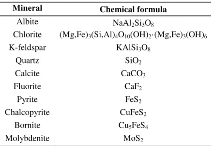
The QMA maps were taken with a spatial resolution and scanning step of 3 μm. Each QMA map is a detailed image where each pixel represents a single mineral at a single position on the sample. A set of 10 relevant mineral phases shown in Table 1 was selected for LIBS identification and quantification.
Table 1 - Selected mineral phases for LIBS quantification.
Mineral Chemical formula
Albite NaAl2Si3O8
Chlorite (Mg,Fe)3(Si,Al)4O10(OH)2·(Mg,Fe)3(OH)6
K-feldspar KAlSi3O8 Quartz SiO2 Calcite CaCO3 Fluorite CaF2 Pyrite FeS2 Chalcopyrite CuFeS2 Bornite Cu5FeS4 Molybdenite MoS2
2.2 LIBS measurements on rock tiles
Laser-induced breakdown spectroscopy (LIBS) is a well-known technique used to obtain elemental information from a sample. To perform a LIBS measurement, a short laser pulse is sent and focused onto a sample surface. The surface is heated by the laser pulse, a portion of the surface’s material is vaporized, and the gas is transformed into plasma. The plasma composition is expected to be representative of the sample’s elemental content. The excited electrons in the upper atomic levels return to lower energy levels, some of them through radiative pathways, emitting photons with narrow distributions of energies. The emitted photons are collected and sent to a spectrometer to produce optical emission spectra associated to the chemical composition of the sample.
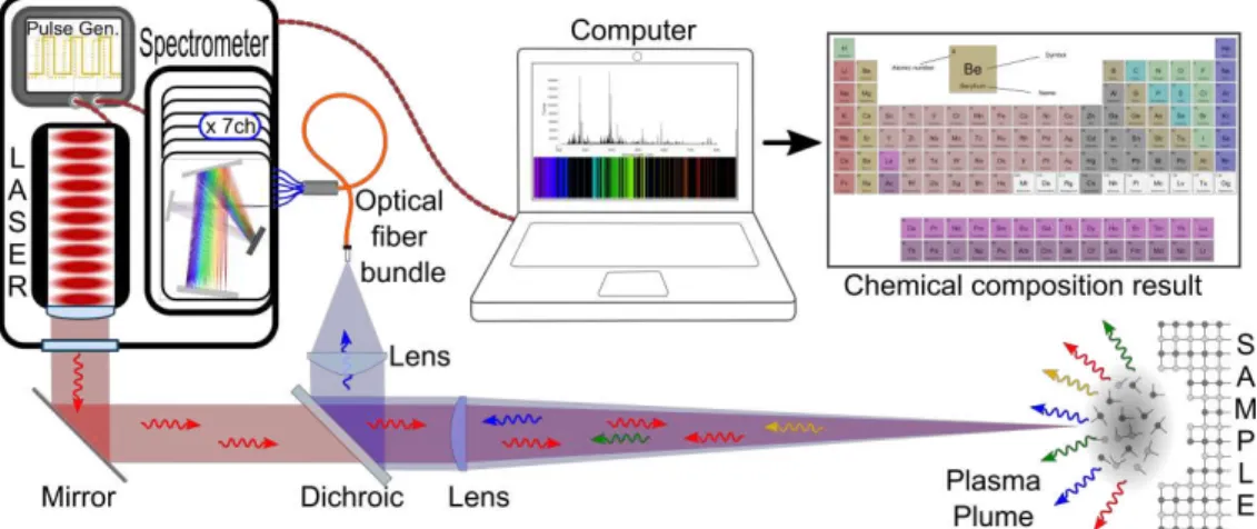
In this work, the rock tiles were placed on top of a 3-axis motorized translation stage and the laser beam was focused onto the sample’s surface using a 250-mm focal-length lens. A Spectra Physics QuantaRay GCR150 Q-switched Nd:YAG of 1064 nm wavelength was operated at a 5 Hz repetition rate and pulse duration of 8 ns, with pulses of 12-mJ energy at the sample’s surface. The emission from the generated plasma light was reflected by a dichroic mirror and collected by a 90-mm focal-length achromatic lens which injected the light into an optical fibre bundle. The optical fibre bundle relayed the light to 7 CCD-spectrometers which covered a wide spectral range (190 – 950 nm) with a resolution around 0.10 nm (UV-visible) to 0.29 nm (IR). A simplified diagram of the LIBS setup is shown in Figure 2.
6
Figure 2 - LIBS setup for mineral identification and quantification on rocks.
A laser spot diameter of 70 μm at the sample was chosen to measure as few mineral phases as possible within the ablation region, whilst still being large enough for field applications. Three LIBS measurements were performed at each spatial position and data analysis was done using the average of the three spectra. A total of 83 samples, each consisting of a 20 × 20 square grid of points spaced by 100 μm were measured by LIBS. The resulting data was grouped into the 83 maps containing 20 × 20 hyperspectral pixels.
2.2.1 LIBS spectra of the studied minerals
Figure 3 shows similar spectra for similar atomic composition of minerals such as (A) silicates, (B) sulfides such as bornite, pyrite and chalcopyrite, and (C) minerals rich in calcium such as fluorite and calcite. However, some dissimilarities in the spectral profiles of these compounds with similar elemental composition can be found. For instance, one can observe:
- Na lines with high intensities for albite, or K lines with high intensities for k-feldspar (A); - different proportions between Cu and Fe lines for bornite and chalcopyrite (B);
- the presence of CaF bands in fluorite mineral around 535 and 602 nm (C).
Separation of pure minerals is possible by using a pattern recognition method, but the quantification of minerals from a mixture of minerals requires a decomposition method, such as the multivariate curve resolution – alternating least squares method (MCR-ALS).
7 (A)
(B)
(C)
Figure 3 – LIBS spectra of pure minerals from tiles measurements. (A) k-feldspar, albite, chlorite and quartz. (B) bornite, pyrite, and chalcopyrite. (C) fluorite and calcite.
3
Data analysis
3.1 Multivariate curve resolution – alternating least squares for LIBS imaging
Given the measurement constraints of an online and real-time LIBS analyzer, the LIBS laser spot area is usually larger than the average grain size of a single mineral phase. Therefore, the LIBS spectrum at a given measured location often contains data of a mixture of several mineral phases. MCR-ALS is well suited to estimate the proportion of each mineral from the mixed spectrum.
8
MCR-ALS is an iterative multivariate self-modeling curve resolution method, and it is applied to recover the response profile of pure components in a mixed spectrum.
The steps to perform MCR-ALS are described in detail in the literature (Tauler, 1995; Zhang and Tauler, 2013). MCR-ALS decomposes the dataset D of size (m × n), which here represents the total LIBS spectra acquired from the measured sample, into two smaller matrices C of size (m ×
k) and ST of size (k × n). m is the number of total spectra and n is the number of variables, i.e. wavelengths. The matrix C contains the abundance profiles of the k pure components i.e. mineral phases, ST is the spectral signature matrix of the individual mineral phases present in the sample. This decomposition can be defined by
D = CST + R , (1)
where R is the residual matrix containing the residual of the final decomposition.
Here, it was critical that MCR-ALS analysis does not output a low number of detected pure components k, avoiding rank deficiency (Amrhein et al., 1996). Rank deficiency can take place in a number of situations, for example when two mineral phases have similar chemical components and identical LIBS spectra, or when a single mineral phase is always correlated to another one. In these cases, the separation of two chemical components is complicated. To solve the rank deficiency issue, we augmented the dataset D to cover different maps on different heterogeneous rock tiles to obtain highly representative data that lead to optimum C and ST matrices. The PLS_Toolbox (v. 8.6, Eigenvector Research, Inc.) software is used to implement the MCR-ALS method.
Even though MCR-ALS is an unsupervised method, QMA data are used for the selection of different mineral phases found in the measurement maps and to associate a physical meaning to the C and ST matrices. After the optimum model is built by the non-supervised MCR-ALS, the QMA and LIBS calibration dataset measured at the same spatial positions are compared to validate the model. Furthermore, to test the generality and the performance of the MCR-ALS model, a test dataset consisting of LIBS data that were not used for the model calibration is chosen to be analyzed and compared with its associated QMA dataset.
3.2 LIBS data analysis
From the 83 maps measured by LIBS, a dataset of 44 maps was used as the calibration set. The remaining 39 maps were used as a test set. MCR-ALS was applied to the calibration set to determine the mineral abundances at each spatial position. The data was pre-processed by spectrum area normalization to compensate the effects of laser energy variation, and closure and non-negativity were selected as constraints. Closure is applied to obtain quantitative information ranging from 0 % to 100 %. Thus, mineral abundances within the LIBS spot areas have values ranging from 0 % to 100 % in the calibration set. Non-negativity is applied to force positive abundance values and positive pure spectrum signatures similar to pure component signatures obtained by LIBS. The number of selected inputs was eleven: ten were attributed to specific known mineral phases (Table 1) and the eleventh, named as “Others”, was for mineral phases not in the mineral phase list.
9
The accuracy of prediction was evaluated using the root mean square error (RMSE), the absolute error, and the maximum error as follows:
RMSE = √∑��= ��Q −��I S
� , (2)
Abs. Error � = |��Q − ��I S| , (3)
Max. Error = max |��QMA− ��LIBS| , (4)
where yiQMA and yiLIBS are respectively the QMA and predicted LIBS abundances, and N is the
number of maps in the dataset.
The quality of the prediction of mineral phases was assessed by the sensitivity and the specificity. In the present context, sensitivity measures the ability of the technique to correctly detect the proper mineral phase, while specificity determines how the model is able to correctly predict that a given observation does not belong to a specific mineral phase.
4
Results and discussions
4.1 Quantitative imaging – calibration set
In LIBS data analysis, the extracted spectral signatures from the matrix ST provide information linked to a set of possible mineral phases. Here, the results of the matrix C determined by MCR-ALS are presented. The matrix C corresponds to the mineral abundance for a specific mineral phase signature in ST.
The 44 LIBS mineral abundance maps predicted for the calibration set are merged together and are shown in Figure 4. QMA mineral abundance was calculated for each spatial position measured by LIBS, by adding the values of the QMA pixels within the LIBS spot area. Thus each mineral abundance map obtained by LIBS has a corresponding map obtained by QMA. The QMA mineral abundance maps were also merged and they are shown in Figure 5. In both cases the pixel color represents the mineral of highest abundance at the given pixel, and the color gradient represents its abundance value. The mineral distribution measured by LIBS is in good agreement with the QMA mineral distribution used as reference.
10
11
Figure 5 - Modified QMA mineral abundance image associated to the calibration set for 10 mineral phases.
The results show a good separation between chalcopyrite (CuFeS2) and bornite (Cu5FeS4) even
though these mineral phases have the same elements in their composition. Moreover, the silicates minerals quartz, k-feldspar, chlorite, and albite, are detected and separated from other silicates known to be present in the samples, included in “Others”. Furthermore, fluorite (CaF2) and
calcite (CaCO3) are both highly rich in calcium and are also detected and discriminated. The
comparison of maps centered at (x,y) = (50,30) in Figure 4 and Figure 5 shows a spatial overestimation of pyrite and an underestimation of albite. Pyrite overestimation may be due to differences of the probed depth by EDS-SEM and by the three LIBS shots.
4.2 Modal mineralogy correlation – calibration set
While the results shown in the preceding section are useful for a visual comparison of LIBS and QMA results for dominant mineral abundances per pixel, the 2D images are a partial representation of the multidimensional data. In this section, the abundances of all ten mineral phases obtained by QMA and LIBS are compared. A range of abundances is obtained by treating each map separately. This study aims at obtaining a quantitative analysis of each map by LIBS, and to compare it to its corresponding QMA map. The mineral abundances obtained by LIBS and QMA, for each map and each mineral are compared and shown in Figure 6. A linear curve
12
fit and its coefficient of determination R2 are obtained for each curve. The obtained R2, maximum error and RMSE are summarized in Table 2. The results show that all the ten mineral phases have a reasonable to high correlation between LIBS and QMA values for the calibration set. R² = 0.85 0 20 40 60 80 100 0 20 40 60 80 100 A b u n d an ce b y LIB S ( % ) Abundance by QMA (%)
(A) K-feldspar
R² = 0.71 0 5 10 15 20 25 0 10 20 30 A b u n d an ce b y LIB S ( % ) Abundance by QMA (%)(B) Albite
R² = 0.69 0 5 10 15 20 25 30 0 5 10 15 20 A b u n d an ce b y LIB S (% ) Abundance by QMA (%)(C) Chlorite
R² = 0.88 0 20 40 60 80 100 0 20 40 60 80 100 A b u n d an ce b y LIB S (% ) Abundance by QMA (%)(D) Quartz
R² = 0.95 0 5 10 15 20 25 0 5 10 15 20 A b u n d an ce b y LIB S (% ) Abundance by QMA (%)(E) Fluorite
R² = 0.96 0 10 20 30 40 50 60 70 80 0 20 40 60 80 A b u n d an ce b y LIB S (% ) Abundance by QMA (%)(F) Calcite
13
Figure 6 - Calibration set comparison of LIBS analysis to QMA data for k-feldspar, albite,
chlorite, quartz, fluorite, calcite, molybdenite, bornite, chalcopyrite, and pyrite. Table 2 - Evaluation of mineral quantitative analysis by LIBS on the calibration set.
Mineral phases R2 Max. Error (%) RMSE (%)
K-Feldspar 0.85 20.8 9.8 Albite 0.71 16.5 4.5 Chlorite 0.69 15.5 3.9 Quartz 0.88 25.0 8.7 Fluorite 0.95 7.5 1.7 Calcite 0.96 5.9 2.5 Molybdenite 0.92 0.5 0.1 Bornite 1.00 8.2 1.4 Chalcopyrite 0.90 10.2 2.7 Pyrite 0.95 6.0 0.9
The correlation presented on Figure 6A shows the ability to quantify K-feldspar. The large number of points in the upper right corner of Figure 6A is explained by the fact that K-feldspar is an abundant mineral in the analyzed samples. Quartz (Figure 6D) was also found to be an abundant mineral phase in the samples, with some maps presenting up to 80 % abundance of this mineral phase. R² = 0.92 0 0.5 1 1.5 2 2.5 0 0.5 1 1.5 2 A b u n d an ce b y LIB S (% ) Abundance by QMA (%)
(G) Molybdenite
R² = 1.00 0 20 40 60 80 100 0 50 100 150 A b u n d an ce b y LIB S (% ) Abundance by QMA (%)(H) Bornite
R² = 0.90 0 10 20 30 40 50 0 10 20 30 40 A b u n d an ce b y LIB S (% ) Abundance by QMA (%)(I) Chalcopyrite
R² = 0.95 0 5 10 15 20 25 30 0 10 20 30 A b u n d an ce b y LIB S (% ) Abundance by QMA (%)(J) Pyrite
14
The map centered at (x,y) = (50,30) in the Figure 4 and Figure 5 was removed as an outlier since it was observed to underestimate albite abundance. Albite underestimation was due to a spatial quasi-omnipresence of pyrite in that map. Both chlorite and albite are less abundant than K-feldspar and quartz, and their RMSE is below 5 % as shown on Table 2. The LIBS results show an agreement with QMA, even though silicates have few lines and all are Si-matrix.
The quantitative analysis is better for fluorite than for silicates. Fluorite presents lower RMSE and higher coefficient of determination than those of silicates, therefore fluorite prediction has a better specificity than silicates. Figure 6E shows a high correlation of LIBS fluorite values against QMA fluorite values within a limited application domain from 0 % to 15 %, and a small dispersion of points at low abundance values, indicating a good sensitivity for fluorite determination, superior to that found in silicate determination. The same conclusion can be drawn for the sensitivity and specificity of calcite determination. Figure 6F shows a good correlation between the predicted values of calcite by LIBS and QMA and the obtained RMSE is 2.5 %. Sulfide mineral prediction also showed a high potential for quantification by LIBS. Figure 6G and Table 2 show a good sensitivity for molybdenite, whose abundance in the calibration set is below 2 %. For bornite, a highly linear correlation was found between the LIBS and QMA results, as shown in Figure 6H. This result is particularly impressive given the high similarity of bornite to chalcopyrite and pyrite. The results for chalcopyrite also confirm a good prediction specificity and sensitivity, especially considering the presence of other sulfides. The presence of pyrite in these tiles is low; however, a good correlation of pyrite is obtained by LIBS and QMA, with no false pyrite prediction.
4.3 LIBS point-counting – calibration set
The previous imaging approach is relevant for determining the accuracy of mineral determination by LIBS compared to a reference imaging method, or to determine mineral texture. However, to determine the mineral abundance of a given surface, the spatial information is irrelevant and only a representative number of measurement points distributed over the given surface is required. The number of measuring points required depends on the mineral content values to be measured. Similarly to point-counting methods, the quantification of a given mineral phase is determined by the ratio of the number of measurement points where the mineral phase is detected over the total number of measurement points. For LIBS measurements, mineral quantification is also performed within each measurement because a larger spot size usually covers more than one mineral phase, and the phase abundances are determined in a single measurement.
For a large number of measurements, the counting uncertainty and confidence level are determined by the binomial standard error and the normal distribution approximation (Howarth, 1998; International Organization for and Technical Committee Iso/Tc, 1994). For example, if pyrite is observed in 100 measurements from a total of 10 000 points, and covers the entire measurement spot size, one can estimate that pyrite covers 1 ± 0.1 % of the given area with a confidence level of 95 %. In our case, a lower counting uncertainty than the example is achieved since the 44 maps of the calibration set totalize 17 600 different spatial locations.
15
The results of the modal analysis performed by LIBS and QMA on the calibration set are shown on Table 3. The difference of the values obtained by LIBS and QMA are assigned as an absolute error, and are shown in the last column of Table 3. This difference is lower than 3 % for the 10 mineral phases analyzed.
Table 3 - Modal analysis on the calibration set.
Mineral phases Abundance (%) Absolute Error
(%)
LIBS Prediction QMA
K-Feldspar 44.1 46.5 2.4 Albite 6.0 7.7 1.7 Chlorite 5.6 5.0 0.6 Quartz 20.5 18.4 2.0 Fluorite 2.3 1.7 0.6 Calcite 6.9 5.6 1.3 Molybdenite 0.1 0.0 0.0 Bornite 5.1 5.3 0.2 Chalcopyrite 4.3 3.7 0.6 Pyrite 0.9 0.8 0.1 Others 4.1 5.1 1.0
16 4.4 Quantitative imaging – test set
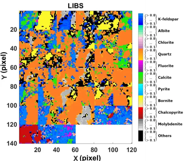
Generalization of the prediction model is based on the prediction of a test set, an unknown dataset of representative size. The test set was processed by the model trained using the calibration set, in order to validate the model’s ability to detect and quantify mineral phases on unknown tiles. The test set contained 39 maps of 20 × 20 pixels. The mineral abundance image is presented in Figure 7 and compared to the QMA quantitative results of Figure 8. The predicted mineral abundance of each LIBS pixel is in good agreement with the reference QMA values, confirming the model quantification ability.
17
18 4.5 Modal mineralogy correlation – test set
The accuracy level of the LIBS prediction was evaluated by comparing the mineral abundances obtained by LIBS to those obtained by QMA on each map. This comparison is performed for each mineral phase and is shown in Figure 9, and a summary is shown in Table 4.
R² = 0.93 0 10 20 30 40 50 60 70 80 0 20 40 60 80 A b u n d an ce b y LIB S (% ) Abundance by QMA (%)
(A) K-feldspar
R² = 0.84 0 5 10 15 20 25 0 10 20 30 40 A b u n d an ce b y LIB S (% ) Abundance by QMA (%)(B) Albite
R² = 0.99 0 2 4 6 8 10 12 14 16 0 5 10 15 20 25 A b u n d an ce b y LIB S (% ) Abundance by QMA (%)(C) Chlorite
R² = 0.94 0 20 40 60 80 100 120 0 20 40 60 80 100 A b u n d an ce b y LIB S (% ) Abundance by QMA (%)(D) Quartz
R² = 0.83 0 2 4 6 8 10 12 14 0 2 4 6 8 A b u n d an ce b y LIB S (% ) Abundance by QMA (%)(E) Fluorite
R² = 0.96 0 10 20 30 40 50 0 10 20 30 40 A b u n d an ce b y LIB S (% ) Abundance by QMA (%)(F) Calcite
19
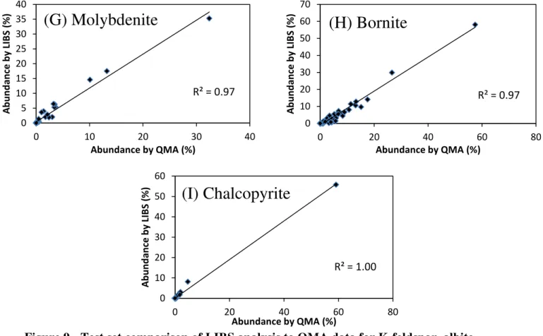
Figure 9 - Test set comparison of LIBS analysis to QMA data for K-feldspar, albite, chlorite, quartz, fluorite, calcite, molybdenite, bornite, and chalcopyrite. No pyrite was present in the QMA data.
Table 4 - Evaluation of mineral quantitative analysis by LIBS on the test set.
Mineral phases R2 Max. Error (%) RMSE (%)
K-Feldspar 0.93 11.3 6.0 Albite 0.84 12.6 2.9 Chlorite 0.99 6.1 1.5 Quartz 0.95 16.6 7.3 Fluorite 0.83 6.4 1.2 Calcite 0.96 10.8 3.7 Molybdenite 0.97 4.5 1.5 Bornite 0.97 5.5 2.1 Chalcopyrite 1.00 3.4 0.8 Pyrite - 0.1 0.0
As shown in Table 4, quality of K-feldspar quantification is conserved even though the model applied to a different dataset than the dataset used for the model calibration. The RMSE did not increase compared to the values obtained for the calibration set. Albite shows similar prediction to the results obtained in the calibration set. Chlorite abundances, as well as quartz abundances predicted by LIBS are also linearly correlated to those obtained by QMA. In conclusion, these
R² = 0.97 0 5 10 15 20 25 30 35 40 0 10 20 30 40 A b u n d an ce b y LIB S (% ) Abundance by QMA (%)
(G) Molybdenite
R² = 0.97 0 10 20 30 40 50 60 70 0 20 40 60 80 A b u n d an ce b y LIB S (% ) Abundance by QMA (%)(H) Bornite
R² = 1.00 0 10 20 30 40 50 60 0 20 40 60 80 A b u n d an ce b y LIB S (% ) Abundance by QMA (%)(I) Chalcopyrite
20
silicates are well quantified by LIBS, as observed in the comparison to the values obtained by QMA.
Figure 9E and Figure 9F show a good quantification sensitivity and specificity for fluorite and calcite. A linear correlation is presented between LIBS and QMA. The same can be concluded for molybdenite. The prediction on the test set conserved a good specificity and sensitivity for bornite and chalcopyrite. Pyrite is predicted in the test set as being not present. As a matter of fact, QMA data showed that this test set does not contain pyrite.
In conclusion, applying our prediction model showed a good agreement between LIBS and QMA results.
4.6 Single-shot LIBS point counting – test set
In the previous section, the LIBS spectrum at a given spatial location was the average of three LIBS measurements at the same position. However, for industrial applications, it is relevant to test whether a single LIBS shot is enough to correctly quantify the mineral content within the LIBS spot area.
To evaluate the mineral prediction capability of a single LIBS shot, only the first spectrum obtained on each point of the test set was used. For simplicity, the same model used in the previous sections that was trained on the average data of three spectra per point on the calibration set was applied. The total mineral abundances obtained from spectral averages of three LIBS shots and the prediction from the first LIBS shot only are compared and shown in Table 5 for the test set. For the averaged spectra, the predicted values of the 10 mineral phases are in agreement with the reference QMA values, and the absolute errors of single-shot measurements are similar to those of three shot measurements.
The results are also in agreement with the QMA reference value with an absolute error below 4 %. Moreover, the absolute error of the single-shot results and the spectrally averaged ones are similar. Thus, higher spectral noise on single-shot data does not affect the ability to predict and quantify mineral phases.
Table 5 - Summary of mineral predictions of the test set.
Mineral phases QMA (%)
3 LIBS laser shots
average 1
st
LIBS laser shot
Predicted average (%) Abs. Error (%) Prediction average (%) Abs. Error (%) K-Feldspar 21.0 24.8 3.8 24.3 3.3 Albite 3.5 2.7 0.8 2.6 0.9 Chlorite 1.8 1.0 0.8 0.5 1.3 Quartz 48.3 46.7 1.5 47.4 0.9 Fluorite 0.3 0.7 0.4 0.5 0.2 Calcite 6.8 9.6 2.8 8.9 2.1 Molybdenite 2.1 2.8 0.7 2.8 0.7
21 Bornite 6.7 5.5 1.2 5.2 1.5 Chalcopyrite 1.8 1.8 0.0 1.8 0.0 Pyrite 0.0 0.0 0.0 0.0 0.0 Others 7.7 4.3 3.4 5.9 1.8
5
Conclusions
This work demonstrates that LIBS is capable of mineral identification and quantification even when a mixture of mineral phases is measured. The MCR-ALS multivariate analysis method was used in combination with QMA data to build a prediction model. Three different quantification capabilities were successfully tested: quantitative mineral imaging, modal mineralogy, and single-shot point counting. In each case, the results showed a good agreement between the mineral phase quantification by LIBS and by QMA.
The results show that LIBS is a promising QMA tool for direct assessment of mineral content. They also indicate that the above-described technique has the potential to be used in field conditions and could be scalable to higher speeds and larger sample dimensions. This approach would allow performing standoff measurements, with no sample preparation. Furthermore, owing to the inherent flexibility of the LIBS configuration, the system could be used in a broad range of embodiments, from a lab bench microscope to a conveyor belt in mining operations. In this paper, we have demonstrated the unprecedented capability of both mineral identification and quantification by LIBS, in both multiple and single laser shot approaches, in the lab environment. The next step will consist in assessing the actual behavior of the system in real world conditions, such as the influence of the surface roughness of natural rocks or the effect of variations of the lens-to-target surface distance, the dust covering the surface of the rock or water (to name a few), which may affect the expected performance of the method. The work addressing these issues is in progress presently in our laboratory.
Acknowledgements
This work was undertaken under the High Efficiency Mining (HEM) Program of the National Research Council Canada in collaboration with the CRC ORE Optimising Resource Extraction in Australia. The authors would like to acknowledge Dr. Nathan Fox and the University of Tasmania for the rock tile samples and the QMA datasets. The authors also thank Théo Varraz for contributing to part of the LIBS measurements.
22
References
Abou Fadel, M., de Juan, A., Touati, N., Vezin, H., Duponchel, L., 2014. New chemometric approach MCR-ALS to unmix EPR spectroscopic data from complex mixtures. Journal of Magnetic Resonance 248, 27-35. Abou Fadel, M., Zhang, X., de Juan, A., Tauler, R., Vezin, H., Duponchel, L., 2015. Extraction of Pure Spectral Signatures and Corresponding Chemical Maps from EPR Imaging Data Sets: Identifying Defects on a CaF2 Surface Due to a Laser Beam Exposure. Analytical Chemistry 87, 3929-3935.
Amrhein, M., Srinivasan, B., Bonvin, D., Schumacher, M., 1996. On the rank deficiency and rank augmentation of the spectral measurement matrix. Chemometrics and Intelligent Laboratory Systems 33, 17-33.
Angel, S.M., Bonvallet, J., Lawrence-Snyder, M., Pearman, W.F., Register, J., 2016. Underwater
measurements using laser induced breakdown spectroscopy. Journal of Analytical Atomic Spectrometry 31, 328-336.
Baum, W., 2014. Ore characterization, process mineralogy and lab automation a roadmap for future mining. Minerals Engineering 60, 69-73.
Demange, M., 2012. Mineralogy for Petrologists: Optics, Chemistry and Occurrences of Rock-Forming Minerals. CRC Press, Fla.
Dold, B., 2017. Acid rock drainage prediction: a critical review. Journal of Geochemical Exploration 172, 120-132.
El Rak e, M., Rutledge, D.N., Moutiers, G., Sir e , J.B., 7. A alysis of ti e‐resol ed laser‐i du ed reakdo spe tra y ea field‐i depe de t o po e ts a alysis MFICA a d ulti ariate ur e resolution–alternating least squares MCR‐ALS . Jour al of Che o etri s .
Felten, J., Hall, H., Jaumot, J., Tauler, R., de Juan, A., Gorzsás, A., 2015. Vibrational spectroscopic image analysis of biological material using multivariate curve resolution–alternating least squares (MCR-ALS). Nature Protocols 10, 217.
Gu, Y., 2003. Automated scanning electron microscope based mineral liberation analysis an introduction to JKMRC/FEI mineral liberation analyser. Journal of Minerals and Materials Characterization and Engineering 2, 33.
Gu, Y., Schouwstra, R.P., Rule, C., 2014. The value of automated mineralogy. Minerals Engineering 58, 100-103.
Haavisto, O., Kauppinen, T., Hakkanen, H., 2013. Laser-induced breakdown spectroscopy for rapid elemental analysis of drillcore. IFAC Proceedings Volumes (IFAC-PapersOnline) 15, 87-91.
Hahn, D.W., Omenetto, N., 2010. Laser-induced breakdown spectroscopy (LIBS), part I: review of basic diagnostics and plasma–particle interactions: still-challenging issues within the analytical plasma community. Applied spectroscopy 64, 335A-366A.
Hahn, D.W., Omenetto, N., 2012. Laser-induced breakdown spectroscopy (LIBS), part II: review of instrumental and methodological approaches to material analysis and applications to different fields. Applied spectroscopy 66, 347-419.
Han, D., Kim, D., Choi, S., Yoh, J.J., 2017. A Novel Classification of Polymorphs Using Combined LIBS and Raman Spectroscopy. Current Optics and Photonics 1, 402-411.
Harhira, A., El Haddad, J., Blouin, A., Sabsabi, M., 2018. Rapid Determination of Bitumen Content in Athabasca Oil Sands by Laser-Induced Breakdown Spectroscopy. Energy & Fuels 32, 3189-3193. Harmon, R.S., Hark, R.R., Throckmorton, C.S., Rankey, E.C., Wise, M.A., Somers, A.M., Collins, L.M., 2017a. Geochemical Fingerprinting by Handheld Laser-Induced Breakdown Spectroscopy. Geostandards Geoanalytical Res. 41, 563-584.
Harmon, R.S., Hark, R.R., Throckmorton, C.S., Rankey, E.C., Wise, M.A., Somers, A.M., Collins, L.M., 7 . Geo he i al Fi gerpri ti g y Ha dheld Laser‐I du ed Breakdo Spectroscopy. Geostandards and Geoanalytical Research 41, 563-584.
23 Harmon, R.S., Remus, J., McMillan, N.J., McManus, C., Collins, L., Gottfried, J.L., DeLucia, F.C., Miziolek, A.W., 2009. LIBS analysis of geomaterials: Geochemical fingerprinting for the rapid analysis and discrimination of minerals. Applied Geochemistry 24, 1125-1141.
Hawthorne, F.C., 1988. Spectroscopic Methods in Mineralogy and Geology. Mineral Society of America. Howarth, R.J., 1998. Improved estimators of uncertainty in proportions, point-counting, and pass-fail test results. American Journal of Science 298, 594-607.
Hugelier, S., Vitale, R., Ruckebusch, C., 2018. Edge-Preserving Image Smoothing Constraint in Multivariate Curve Resolution–Alternating Least Squares (MCR-ALS) of Hyperspectral Data. Applied Spectroscopy 72, 420-431.
International Organization for, S., Technical Committee Iso/Tc, S.m.f., 1994. Methods for the petrographic analysis of bituminous coal and anthracite. Method of determining maceral group composition Part 3 Part 3. International Organization for Standardization, Geneva, Switzerland.
Khajehzadeh, N., Kauppinen, T.K., 2015. Fast mineral identification using elemental LIBS technique. IFAC-PapersOnLine 48, 119-124.
Moncayo, S., Duponchel, L., Mousavipak, N., Panczer, G., Trichard, F., Bousquet, B., Pelascini, F., Motto-Ros, V., 2018. Exploration of megapixel hyperspectral LIBS images using principal component analysis. Journal of Analytical Atomic Spectrometry 33, 210-220.
Newbury, D.E., Ritchie, N.W.M., 2013. Is Scanning Electron Microscopy/Energy Dispersive X-ray Spectrometry (SEM/EDS) Quantitative? Scanning 35, 141-168.
Noll, R., 2012. Laser-induced breakdown spectroscopy, Laser-Induced Breakdown Spectroscopy. Springer, pp. 7-15.
Parbhakar-Fox, A.K., Edraki, M., Walters, S., Bradshaw, D., 2011. Development of a textural index for the prediction of acid rock drainage. Minerals Engineering 24, 1277-1287.
Qiao, S., Ding, Y., Tian, D., Yao, L., Yang, G., 2015. A Review of Laser-Induced Breakdown Spectroscopy for Analysis of Geological Materials. Applied Spectroscopy Reviews 50, 1-26.
Rifai, K., Laflamme, M., Constantin, M., Vidal, F., Sabsabi, M., Blouin, A., Bouchard, P., Fytas, K., Castello, M., Kamwa, B.N., 2017. Analysis of gold in rock samples using laser-induced breakdown spectroscopy: Matrix and heterogeneity effects. Spectrochimica Acta Part B: Atomic Spectroscopy 134, 33-41. Smith, J.P., Smith, F.C., Booksh, K.S., 2018. Multivariate Curve Resolution–Alternating Least Squares (MCR-ALS) with Raman Imaging Applied to Lunar Meteorites. Applied Spectroscopy 72, 404-419. Tauler, R., 1995. Multivariate curve resolution applied to second order data. Chemometrics and intelligent laboratory systems 30, 133-146.
Washburn, K.E., 2015. Rapid geochemical and mineralogical characterization of shale by laser-induced breakdown spectroscopy. Organic Geochemistry 83, 114-117.
Wiens, R., Maurice, S., Lasue, J., Forni, O., Anderson, R., Clegg, S., Bender, S., Blaney, D., Barraclough, B., Cousin, A., 2013. Pre-flight calibration and initial data processing for the ChemCam laser-induced breakdown spectroscopy instrument on the Mars Science Laboratory rover. Spectrochimica Acta Part B: Atomic Spectroscopy 82, 1-27.
Yelameli, M., Thornton, B., Takahashi, T., Weerkoon, T., Takemura, Y., Ishii, K., 2016. Support vector machine based classification of seafloor rock types measured underwater using Laser Induced Breakdown Spectroscopy, OCEANS 2016-Shanghai. IEEE, pp. 1-4.
Zhang, X., Tauler, R., 2013. Application of multivariate curve resolution alternating least squares (MCR-ALS) to remote sensing hyperspectral imaging. Analytica chimica acta 762, 25-38.