Characterization of higher-order scattering from vegetation with SMAP measurements

Characterization of higher-order scattering

from vegetation with SMAP measurements

The MIT Faculty has made this article openly available.

Please share

how this access benefits you. Your story matters.

Citation

Feldman, Andrew F., Ruzbeh Akbar, and Dara Entekhabi.

"Characterization of higher-order scattering from vegetation with

SMAP measurements." Remote Sensing of Environment, 219, 15

(December 2018): 324-338. © 2018 The Author(s)

As Published

http://dx.doi.org/10.1016/j.rse.2018.10.022

Publisher

Elsevier BV

Version

Final published version

Citable link

https://hdl.handle.net/1721.1/125694

Terms of Use

Creative Commons Attribution 4.0 International license

Contents lists available atScienceDirect

Remote Sensing of Environment

Characterization of higher-order scattering from vegetation with SMAP

measurements

Andrew F. Feldman

_{, Ruzbeh Akbar, Dara Entekhabi}

Department of Civil and Environmental Engineering, Massachusetts Institute of Technology, Cambridge, MA 02139, United States

A R T I C L E I N F O

Keywords:

Soil moisture

Passive microwave radiometry SMAP

Multiple-scattering

A B S T R A C T

Vegetation cover absorbs and scatters L-band microwave emission measured by SMOS and SMAP satellites. Misrepresentation of this phenomena results in uncertainties when inferring, for instance, surface soil moisture in retrieval algorithms that commonly utilize the tau-omega model which is most applicable for a weakly scattering medium. In this study, we investigate the degree to which multiple-scattering is prevalent over a range of land cover classifications (from lightly vegetated grasslands to dense forests) at the satellite scale by explicitly accounting for multiple-scattering in a first-order radiative transfer model, developed here. Even though the tau-omega model with effective parameters can possibly capture higher-order scattering contributions, deliberately partitioning scattering into different components is required to estimate multiple-scattering properties. Specifically, we aim to determine how one can partition between zeroth and first-order radiative transfer terms within a retrieval algorithm without ancillary information, determine whether this method can detect first-order scattering at the SMAP measurement scale without ancillary information, and quantify the magnitude of de-tected scattering. A simplified first-order radiative transfer model which characterizes single interactions of microwaves with a scattering medium is developed for implementation within retrieval algorithms. This new emission model is implemented within a recently developed retrieval algorithm, the multi-temporal dual channel algorithm (MT-DCA), which does not require ancillary land use information. Scattering parameters as well as SM and vegetation optical depth (τ) are retrieved simultaneously in Africa and South America using the first year of SMAP brightness temperature measurements on a 36 km grid. Specifically, an introduced time invariant first-order scattering coefficient (ω1) is retrieved representing microwave emission interaction with the

canopy. We find that ω1is typically zero in lightly vegetated biomes and non-zero (~0.06) in 74% of the forest

pixels. In forest-dominated pixels, the median first-order emissivity is 0.04, or about 4.3% of a given SMAP radiometer brightness temperature measurement. Additionally, explicitly accounting for first-order scattering terms in the radiative transfer model tends to increase SM and τ retrievals by a median of 0.02 m3_/m3_{and 0.1,}

respectively, only in forested regions. This study demonstrates the first attempt to explicitly partition higher-order scattering terms in a retrieval algorithm at a satellite scale and ultimately provides a fundamental un-derstanding and quantification of multiple-scattering from grasslands to forests.

1. Introduction

Vegetation can play a major role in regulating surface fluxes espe-cially in regions with more active terrestrial water, energy, and carbon cycles. This photosynthetic activity is often sensitive to the root-zone water availability stored in the surface below. Thus, accurately quan-tifying surface soil moisture (SM), especially for vegetated surfaces, is critical to understanding the coupling of these cycles at the land surface with implications for global carbon cycle monitoring and weather forecasting, for instance. Due to spatial heterogeneity of the surface, it is impractical to monitor SM over large areas with ground networks.

The ESA Soil Moisture and Ocean Salinity (SMOS; launched 2009) (Kerr et al., 2010) and NASA Soil Moisture Active Passive (SMAP; launched 2015) (Entekhabi et al., 2010) satellites provide global measurements of Earth's passive microwave emission at L-band (1.4 GHz) with the goal of retrieving surface SM (top 5 cm). This retrieval is possible due to low frequency microwave emission sensitivity to soil dielectric prop-erties (directly related to SM). While low frequency microwaves origi-nating from the surface can largely penetrate light vegetation, they are significantly attenuated and subject to multiple-scattering in the pre-sence of denser vegetation including vegetation components of di-mensions comparable to the observation wavelength, specifically 21 cm

https://doi.org/10.1016/j.rse.2018.10.022

Received 2 May 2018; Received in revised form 8 September 2018; Accepted 14 October 2018

⁎_{Corresponding author.}

E-mail address:afeld24@mit.edu(A.F. Feldman).

Remote Sensing of Environment 219 (2018) 324–338

Available online 23 October 2018

0034-4257/ © 2018 The Authors. Published by Elsevier Inc. This is an open access article under the CC BY license (http://creativecommons.org/licenses/BY/4.0/).

for L-band (Ulaby and Long, 2014). This hinders accurate monitoring of

SM under moderate to heavy vegetation, especially in forests which

comprise approximately 30% of Earth's terrestrial biosphere and sig-nificantly influence global biogeochemical cycles (Nemani et al., 2003). In this study, we investigate the significance of multiple-scattering across a range of vegetation types from grasslands to forests. We do this by retrieving time-varying soil moisture and vegetation optical depth (τ) as well as scattering parameters (i.e., ω and ω1; discussed later) from

SMAP measurements without ancillary information.

Numerous field campaigns evaluated the effects of forest cover on passive microwave emission (Pampaloni, 2004). Aircraft microwave emission measurements of various land cover types show that the presence of canopy cover attenuates the below soil emission (Shutko, 1982) and thus reduces SM sensitivity (Ulaby et al., 1983). These findings were later confirmed with ground measurements (Guglielmetti et al., 2008, 2007;Mätzler, 1994). Specifically, it was determined that primary tree branches are the most significant attenuators (over leaves and trunks) of low-frequency microwave emission (Chauhan et al., 1991;Ferrazzoli and Guerriero, 1996;Macelloni et al., 2001;Mätzler, 1994). While the difficulty of separating out the bare surface signal is evident especially with the presence of leaf litter (Grant et al., 2007; Schwank et al., 2008), low frequency microwave radiometers are in fact sensitive to SM in forests (Chauhan, 1999;Della Vecchia et al., 2010; Lang et al., 2001).

In SM retrieval applications using radiometers, in order to char-acterize upwelling surface and vegetation emission, the passive mi-crowave remote sensing community commonly uses the zeroth-order solution to the scalar radiative transfer (RT) equations. This is often referred to as the tau-omega model (Mo et al., 1982). For instance, the SMOS retrieval algorithm currently uses the L-MEB inversion approach (Wigneron et al., 2017, 2007) which utilizes this RT model to determine

SM and τ, which was determined to be linearly proportional to

vege-tation water content (VWC) (Jackson and Schmugge, 1991). Ad-ditionally, the SMAP baseline retrieval approach also uses the tau-omega model to estimate SM (O'Neill et al., 2015). This zeroth-order RT approach considers the vegetation layer to be an attenuating medium, thus neglecting higher order multiple-scattering effects within the ca-nopy. Therefore, it is theoretically an insufficient representation of canopy volume scattering when canopy constituents approach or ex-ceed the measurement wavelength (e.g., 21 cm at L-band) which is the case in forests (Kurum et al., 2012). As a consequence, both the SMOS and SMAP missions flag SM retrievals under heavy vegetation, speci-fically when VWC exceeds 5 kg/m2_{, noting likely reduced accuracy.}

It has been shown that the zeroth-order RT model in its analytical form can, using effective parameters, account for multiple-scattering (Ferrazzoli et al., 2002; Kurum, 2013). One can calibrate vegetation parameters, specifically τ and single-scattering albedo (ω), using mea-sured canopy information combined with a numerical model (Ferrazzoli et al., 2002). These equivalent τ and ω parameters can be used as initial conditions in retrieval of SM and τ using the zeroth-order RT model (Rahmoune et al., 2014, 2013). This method has recently been im-plemented within the SMOS retrieval algorithm using aircraft and ground measurements to determine τ and ω for use in SM and τ in-version (Rahmoune et al., 2014, 2013;Vittucci et al., 2016). Also, it was demonstrated that ω can be aggregated with theoretical higher-order scattering parameters into an effective ω (Kurum, 2013). Effective ω was recently estimated globally using the zeroth-order RT model and SMAP data without ancillary information (Konings et al., 2017). Other studies demonstrate calibrating microwave vegetation parameters in the zeroth-order RT model to match ground measured emissivity in forests (Saleh et al., 2003; Santi et al., 2009). However, no satellite-based investigation has been conducted in which partitioned multiple-scattering RT terms are explicitly accounted for in the retrieval algo-rithm. Retrieval algorithms in this context are techniques that estimate microwave parameters such as surface roughness (i.e., soil moisture), vegetation optical depth, effective scattering albedo, or combination of

these simultaneously from passive microwave brightness temperature measurements. Thus, the degree to which multiple-scattering is present over different vegetation types is not known at the satellite scale as this cannot be deduced solely from calibrated zeroth-order RT model parameters. Rather, it can be determined explicitly from introduction of order interaction terms within the RT model. However, higher-order interaction terms are currently impractical to implement within RT models used in retrieval algorithms.

Numerous studies developed RT models accounting for higher levels of complexity including surfaces with varying SM and temperature profiles (Njoku and Kong, 1977), grass covered surfaces (Saatchi et al., 1994), random leaf-filled canopy covered surfaces (Wigneron et al., 1993), leaf litter covered surfaces (Schwank et al., 2008), snow covered surfaces (Proksch et al., 2015;Schwank et al., 2014;Wiesmann and Mätzler, 1999), and forest covered surfaces (Ferrazzoli and Guerriero, 1996;Karam, 1997;Kurum et al., 2011;Lang et al., 2001;Macelloni et al., 2001). As the focus of this study is on characterizing vegetation scattering, we summarize the previously developed RT models for for-ests here. These higher-order RT solutions typically model canopy constituents as randomly oriented disks and cylinders. However, their performance rests on accurate representation of canopy geometry, thus requiring extensive model parameterization and in-situ data collection. Specifically,Karam (1997)developed a physical, discrete, numerical RT model which iteratively solves the RT equations. Ferrazzoli and Guerriero (1996)developed a discrete numerical RT model, called the Tor Vergata model, which uses a matrix doubling algorithm to compute emissivity.Lang et al. (2001)modelled a pine stand using the distorted born approximation and Peake's principle to relate active to passive parameters. Macelloni et al. (2001)utilized a discrete element first-order RT model developed byTsang et al. (1985)relying on the bridge and infinite cylinder approximation to compute the scattering ampli-tudes. Finally,Kurum et al. (2011)iteratively solved the RT equations using the zeroth-order solution as an exciting source to obtain the first-order RT equations.

While these models can accurately represent passive microwave interaction with canopy geometry at the forest plot scale, there are computational barriers in implementing them within global scale re-trieval algorithms in the case of SMOS and SMAP. Calibration of zeroth-order RT model parameters at the satellite scale additionally requires a network of in-situ measurements which make assumptions about ap-plicability of measurements at one site to other geographical regions with similar land cover classifications (Ferrazzoli et al., 2002; Saleh et al., 2003;Santi et al., 2009). This provides motivation for a retrieval algorithm that explicitly accounts for higher-order soil-canopy inter-actions with the ability to infer scattering information without ancillary information. Currently, a so called “two-stream” RT model for vege-tated canopies based on the Microwave Emission Model of Layered Snowpacks (MEMLS) developed in Wiesmann and Mätzler (1999)is being tested for use in the SMOS baseline retrieval algorithm (Wigneron et al., 2017).

In this paper, a simple first-order RT model is developed which introduces one additional parameter to account for first-order scat-tering from the vegetation layer. This is the first attempt to explicitly (e.g., adding first-order scattering terms to the tau-omega model) rather than implicitly (e.g., calibrating effective tau-omega model parameters) account for multiple-scattering within a retrieval algorithm at the sa-tellite scale. We integrate the first-order RT model within a multi-temporal dual channel algorithm (MT-DCA) (Konings et al., 2016) to retrieve vegetation scattering parameters as well as time-varying SM and τ over Africa and South America. We are interested in retrieval differences between significantly different land cover classifications (e.g., between grasslands and forests), prevalent in these regions. We do not investigate retrieval differences between specific types of forests here. The approach purposefully avoids use of ancillary data on land use and vegetation characteristics such as those derived from optical and/or in-situ measurements. While first-order SM retrievals are

attempted in this study, we assert that these are not enhanced retrievals as they are not comprehensively validated (as a result of insufficient in-situ SM measurements in more dense or forested regions at the current 40 km L-band radiometer footprint scale). Rather, we focus on in-formation obtained from estimates of vegetation scattering parameters and pose the following research questions. (I) How can a higher-order RT model which explicitly partitions between zeroth and first-order scattering terms be implemented within a retrieval algorithm without requirement of ancillary land cover information? (II) By explicitly partitioning between zeroth and first order scattering terms, can first-order scattering be detected from SMAP polarized brightness tem-perature measurements without ancillary information? (III) If so, what is the magnitude of first-order emission across land cover classifica-tions? (II) and (III) ultimately address whether we can identify areas where a transition from a zeroth-order to first-order RT model might be important.

Section 2reviews the zeroth-order RT model, introduces the first-order RT model, and discusses retrieval algorithm implementation, study region, and datasets.Section 3displays the results of the algo-rithm retrievals of scattering information.Section 4discusses limita-tions of scattering parameter retrieval, limitalimita-tions of retrieval com-parison, and behavior of the proposed first-order RT model. A summary and conclusion section follows inSection 5.

2. Methodology

2.1. Zeroth-order RT (tau-omega) model

The zeroth-order solution to the scalar RT equation is obtained by omitting canopy scattering terms. This approach thus assumes the ve-getation layer acts as an attenuating medium affecting up-welling soil and vegetation emission (Ulaby and Long, 2014). Within the SM remote sensing community, the zeroth-order RT solution is referred to as the tau-omega model and is expressed as:

TB0thp = (1 r Tp) S+ rp(1 )(1 )TC+(1 )(1 )TC (1) where TBpis the total upwelling brightness temperature, the subscript p

is either horizontal (p = H) or vertical (p = V) polarization, γ is trans-missivity of the microwave emission through the vegetation canopy, rp

is the rough surface reflectivity, ω is the single-scattering albedo of the vegetation layer, TSis effective soil physical temperature, and TC is

effective canopy physical temperature. γ and ω are theoretically po-larization dependent, but this dependence is neglected in this study as is often the case in the implementation of the tau-omega model (Kerr et al., 2010;O'Neill et al., 2016a). Note that at the time of the 6 AM SMAP overpass, TSand TCare in approximate thermodynamic

equili-brium requiring only one ancillary measurement of effective surface physical temperature. γ is represented by:

e ( sec )

= ₍₂₎

where θ is the incidence angle relative to nadir (e.g., 40° for SMAP). τ is equal to the extinction coefficient (κe) multiplied by the geometrical

canopy height (d). κeis equal to the addition of the absorption (κa) and

scattering coefficients (κs). Accordingly, ω is the fraction of extinction

due to scattering: s

e =

(3) Finally, the surface reflectivity is commonly modelled as:

rp= pe h cosN (4)

where Γpis the Fresnel specular surface reflectivity, h is the empirically

determined surface roughness coefficient, and N is a model parameter.

Γ_pis related to the soil dielectric constant (ε) which in turn is related to SM and soil texture (Dobson et al., 1985;Mironov et al., 2009).

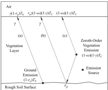
Physically, the terms in Eq.(1)and in order (left to right) represent (a) canopy attenuated surface emission, (b) attenuated, surface re-flected, downward vegetation emission, (c) and upward vegetation emission. These emission pathways are shown inFig. 1. The reflectivity of the air-canopy interface is assumed to be zero (diffuse boundary assumption).

2.2. First-order RT model

Hornbuckle and Rowlandson (2008)andKurum et al. (2011)relax the assumption of weak canopy scattering and solve the scalar RT equations to the first order. That is, an additional single-scattering term is considered when solving the scalar RT equations. In this paper, first-order scattering is defined as an additional surface or vegetation emission term that interacts, or scatters, once from the vegetation medium. This expansion results in Eq.(1)plus an additional first-order scattering term representing different combinations of first-order emission pathways.Fig. 2provides some context for these additional emission pathways. The first-order upwelling emission (originating from both surface and vegetation sources) scatters once from the ca-nopy medium. This scattering can take place at any height within the

Fig. 1. Zeroth-order RT (tau-omega) model emission pathways. Indices (a) to

(c) for emission pathways are defined in the text. Note that “zeroth-order ve-getation emission” is veve-getation source of (1 − ω) multiplied by (1 − γ).

Fig. 2. Schematic representation of zeroth (dashed) and first-order (solid)

emission pathways. Note, this schematic does not include all first-order emis-sion pathways.

vegetation canopy. It is most likely to occur at the location of vegetation structures such as trunks, branches, or dense clusters of green biomass. However, in this study, we assume that this scattering process takes place at only one elevation in order to achieve parsimony that allows global estimation with existing satellite data. For clarity, this is denoted as the first-order scattering centroid and is located at f · d or a fraction (f) of the height of the canopy (d) above the surface.

Iteratively solving the RT solutions to a higher-order through ex-panding and solving the scattering source terms results in an accurate representation of canopy scattering. This approach is nonetheless im-practical to implement within a satellite pixel scale retrieval algorithm. Rather, a ray tracing method is implemented here to account for first-order scattering terms that resemble theoretical terms developed in Kurum et al. (2011)as closely as possible. We ray trace all eight first-order pathways outlined inKurum et al. (2011). Simplifications and assumptions are further required to approximate the theoretical order scattering terms and are developed here. (a) We assume all first-order scattering only takes place at a single height, or the first-first-order scattering centroid shown conceptually inFig. 2. This is in contrast to the assumption that multiple-scattering occurs uniformly throughout the vegetation medium as inKurum et al. (2011). (b) As is the case for the scattering medium inKurum et al. (2011), we assume that the ve-getation medium is azimuthally symmetrical, reciprocal, and homo-genous and scattering occurs at all angles in the upper hemisphere. Further, scattering from the canopy at this centroid is defined by the first-order scattering coefficient, ω1, rather than scattering source

functions in Kurum et al. (2011). (c) Rather than emission from all locations, we assume upward (downward) vegetation emission that is scattered at the first-order scattering centroid is emitted from the bottom (top) of the canopy. (d) For each of the eight possible first-order emission pathways, we assume only one average pathway represents all possible emission pathways at all angles with respect to nadir. This is in lieu of accounting for all possible incidence and scattered angles in the upper hemisphere. In this study, we additionally assume that the first-order scattering centroid is located at one half the canopy height and that the emission within the average pathway traverses the canopy at the specified incidence angle. Thus, assumption (b) is modified in this case such that scattering at the first-order scattering centroid occurs only at the specified incidence angle. However, we show later in this section that these additional assumptions can be relaxed with a more complex representation of the developed RT model. In the context of ray tracing, assumptions (a) and (c) mean that first-order emission pathways that interact with the canopy at this centroid will only be partially attenuated by the vegetation layer. This requires adjustment of Eq.(2)in these cases. When the emission traverses between the first-order scattering centroid and bottom of canopy, the attenuation is re-presented by:

e

f= (f de sec ) (5)

Conversely, f is replaced by 1 − f in Eq. (5)if emission traverses between the first-order scattering centroid and top of canopy. As-sumption (b) states that ω1is isotropic (i.e., angle independent) and

thus upward and downward scattering from the vegetation medium are equal. Additionally, ω1is distinguished from the single-scattering

al-bedo definition in that ω1 can represent scattering over the upper

hemisphere at the first-order scattering centroid and ω represents scattering in all directions from any vegetation constituent in the ve-getation layer.

With these assumptions, the first-order emission pathways are de-veloped as shown inFig. 3. Note that each single microwave interaction with the canopy at the first-order scattering centroid results in two separate first-order scattering terms from downward and upward scat-tering. As an example, consider the two ground emission pathways in Fig. 3A (left). Ground emission occurs with (1 − rp) at the black symbol,

is attenuated by γf_{for traversing f∙d∙sec(θ) through the medium and is}

scattered both upwards and downwards at the first-order scattering

centroid resulting in multiplication by ω1. In the downward scattering

case, it is again attenuated by γf_{, reflected from the surface gaining a}

factor rp, and is fully attenuated by the length of the layer obtaining a

factor γ. This creates one first-order scattering term: ω1rpγ(2f+1)(1 − rp).

In the upward scattering case, the emission is attenuated by γf_creating

another first-order scattering term: ω1γ(1 − rp). Note that the eight

first-order emission terms inFig. 3are in addition to the already ex-isting zeroth-order terms outlined in Eq.(1). Thus, the summation of Eq. (1) and the first-order pathways yields an approximate re-presentation of the solution to the first-order RT equation:

TBpTotal=TBp0th+TBp1st (6)

where TBp0this obtained from Eq.(1)and TBp1stis the first order TBp

emission, obtained by summing the terms inFig. 3. Assuming TSand TC

are in approximate thermodynamic equilibrium and f equals 0.5, viable assumptions used in this study, Eq.(6)can be simplified to:

epTotal=[ea+eb+ec]0th+[ (11 + rp)(ea+ eb+2 ec)]1st (7) where ea is γ(1 − rp) (e.g., zeroth-order ground emission), eb is

γrp(1 − ω)(1 − γ) (e.g., zeroth-order vegetation emission with surface

reflection), and ec is (1 − ω)(1 − γ) (e.g., zeroth-order vegetation

emission). Brackets separate zeroth and first-order terms as noted by the superscripts. Subscripts a, b, and c correspond to zeroth-order emission sources inFig. 1. While only rpis polarization dependent as in

Eq.(1), γ and ω can also be polarization dependent. Note that when first-order scattering is negligible (i.e., ω1= 0), TBp1stbecomes zero

and Eq.(6)is thus equal to Eq. (1). It is worth noting that the for-mulation in Eqs.(6) and (7)is consistent withKurum et al. (2011) first-order RT model such that increased ω causes reduction in TBpTotalwhile

increased first-order scattering (increased ω1) tends to increase TBpTotal

(Kurum, 2013). We use this formulation here to estimate constant va-lues of ω1and ω along with time varying γ and rpsolely from SMAP TBp

measurements. This is in contrast to making use of a numerical model to initially determine scattering parameters from in-situ measurements (Rahmoune et al., 2013) or calibrating an effective ω in the zeroth-order RT model which accounts for multiple-scattering (Kurum, 2013). Note that Eq.(6)can be modified to more precisely represent the canopy height and angle of emission pathways as in the theoretical first-order RT equation. For instance, f can be a random variable which permits more accurate representation of the canopy structure if the vertical distribution of the vegetation structure is known as is the case from localized ground or remote sensing studies (Krofcheck et al., 2016). If the probability density function of f is known and defined as p (f), the expected value of TBpTotalcan be computed by integrating over

all possible scattering centroid heights:

E TB[ pTotal] ₀ p f TB( ) p df

1 _Total

= ₍₈₎

where f is bounded by 0 and 1 and TBpTotalis obtained from Eq.(6).

Based on a sensitivity analyses (discussed further inSection 4.1), we find that other variables in Eq.(6)only marginally depend on f, thus greatly simplifying the integration. In the case of a uniform distribution,

p(f) = 1 in which case Eq.(8)can be solved analytically. A more ver-satile distribution, such as a Beta distribution, is recommended for use as it is bounded between 0 and 1 and distribution skewness can be varied. In this case, Eq.(8)can be solved numerically. In this study however, f is simply assumed to be fully concentrated at half of the height of the canopy (i.e., a Dirac delta function where p (f) = δ(f − 0.5)).

Additionally, θ in Eq.(5)can be generalized as a random variable,

θ′ with probability density function defined as p(θ′), which represents

any angle between −π/2 and π/2 when referring to a segment of an emission pathway not crossing the air-canopy boundary. This can be accomplished again by using the expected value rule given a known distribution of angles of incoming and scattered emission rays:

E[ ]f p( ) fd

2 2

=

(9) This provides the average transmissivity of an emission pathway between the ground and first-order scattering centroid and vice-versa and replaces all γf_{terms inFig. 3. The same can be performed for the}

average transmissivity of an emission pathway between the top of ca-nopy and first-order scattering centroid by replacing f with 1 − f in Eq. (9). This more complex implementation provides a closer comparison to theoretically derived scattering terms in Kurum et al. (2011) which integrates over all possible combinations of incident and scattered emission. If both f and θ′ are assumed as random variables simulta-neously, Eq.(9)must be implemented within Eq.(7)before Eq.(8)is applied. Assuming p(θ′) is a uniform distribution (i.e., p(θ′) = 1 / π), Eq. (9)was solved numerically determining that the average θ′ was between 35° and 55° depending on values of τ and d. Thus, in this study, an effective, constant θ′ at the SMAP incidence angle of 40° (i.e., a Dirac delta function where p(θ′) = δ(θ′ − 2π / 9)) was deemed sufficient to use as in Eq.(9)or simply θ is equal to 40° in Eq.(5).

2.3. Retrieval algorithm

The multi-temporal dual channel algorithm (MT-DCA) was chosen as the retrieval algorithm in this study for its ability to simultaneously retrieve scattering parameters (i.e., ω and ω1), SM, and τ without

an-cillary vegetation information. This algorithm is fully described in Konings et al. (2016), with a summary provided here.Konings et al. (2015)show that horizontally and vertically polarized TBp(measured

by both SMAP and SMOS) are correlated at the SMAP incidence angle of 40° which prevents robust retrieval of two parameters (commonly SM and τ within a dual-channel algorithm). To retrieve multiple para-meters, the MT-DCA circumvents this issue through utilization of TBp

measurements from two consecutive overpasses (separated by

approximately three days) and assumes that vegetation dynamics change slowly between overpasses to retrieve three variables: ε (di-rectly related to SM) from the first and second overpass and constant τ between overpasses. Degrees of information (DOI) provide the frac-tional number of variables that can be estimated from the probability distributions of the measurements. The greater the correlation of measurements, the lower the DOI.Konings et al. (2015)show that the upper limit on DOI for the four TBpmeasurements between consecutive

passes is approximately 3.72 or enough information to robustly retrieve three parameters in most conditions.

The MT-DCA consists of an inner optimization routine which, as-suming a temporally constant ω value, estimates SM and τ using two consecutive SMAP overpasses. This inner-loop minimizes the following objective function: min X , , J X( ) (TB TB ( ))X t p H V p Obs pModel 1 2 ₁ 2 , 2 = = = = (10)

where t is the overpass index, TBpObsis the radiometer measurement

and TBpModelis forward modelled from either the zeroth or first-order

emission models from Eq.(1)or(6), respectively. Essentially, the cost function, J, is minimized by adjusting ε from the two consecutive overpasses (i.e., ε1 and ε2) and the constant τ between passes to fit

TBpModelto TBpObsover both polarizations and both overpasses.

The outer MT-DCA estimation scheme retrieves a temporally con-stant ω through model selection. That is the optimum ω which yields the smallest cost function is chosen. ω is assumed approximately con-stant over a year consistent with previous studies (Konings et al., 2016; Wigneron et al., 2004). The method to obtain ω outlined inKonings et al. (2016) is modified here to additionally retrieve a temporally constant ω1. Thus, the optimization in Eq.(10)is modified to estimate

temporally constant ω and ω1 values over all pairs of consecutive

overpasses:

Fig. 3. First-order emission pathways. 3A: Ground

emission and upward vegetation emission scattering pathways. 3B: Downward vegetation emission scat-tering pathways with and without surface reflection. Note that “zeroth-order vegetation emission” is ve-getation source of (1 − ω) multiplied by (1 − γ). The emission pathways are the same as those inKurum et al. (2011)(see their Fig. 3).

min J min X J X TB TB X , , , ( ) ( ( )) n M t p H V pObs pModel 11 1 1 2 1 2 , 2 = ₌ = = = = (11) where J1is the first-order implementation cost function and M is the

number of overpasses (~120 annually for SMAP at a given location). Notice in Eq.(11)that Eq.(10)is computed M times given one set of constant values for ω and ω1. Refer toKonings et al. (2016)for more

information on the minimization approaches in Eqs.(10) and (11). The MT-DCA is implemented twice. In the first implementation, the original approach outlined inKonings et al. (2016)is utilized which only estimates ω, henceforth referred to as the zeroth-order im-plementation. In this case, ω1is set to 0 in Eq. (11) resulting in J0

(instead of J1) or the zeroth-order implementation cost function. The

second MT-DCA implementation estimates both ω and ω1albedo terms

as in Eq.(11). Note that the retrieved vegetation parameters (τ, ω, and

ω1) are effective rather than theoretical parameters (Kurum, 2013;

Wigneron et al., 2017). However, using the first-order RT model in Eq. (7), retrievals of ω are more closely related to a single-scattering albedo with multiple-scattering effects partitioned into ω1. Estimation of ω in

the aforementioned zeroth-order MT-DCA implementation using Eq.(1) would result in an effective scattering albedo which lumps the effects of the theoretical single-scattering and multiple-scattering effects. Thus, it is expected that ω from the zeroth-order implementation is lower than

ω from the first-order implementation based on results in Kurum (2013). For computational tractability, ω and ω1are discretized into

0.01 increments. ω and ω1are considered constant over a year and are

retrieved in a model selection manner in Eq.(11), therefore effectively requiring fractional DOI per overpass. Thus, we assert that their esti-mates should generally not be subject to optimization instability with unphysical compensation between variables. Additionally, simulations of Eq.(11)revealed that artificial TBpperturbations added to the SMAP

TBpmeasurements used as inputs on the order of 2 K were required to

change ω and ω1by 0.01. These perturbations are greater than SMAP

estimated radiometer noise of 1.1 K (Piepmeier et al., 2016). We do, however, acknowledge a possible reduction in DOI in forests where TBH

and TBVhave greater correlation and smaller difference in magnitudes.

Finally, τ, ω, and ω1are assumed to be polarization independent in

Eq.(11)which reduces the number of retrieved parameters. While this assumption may be insufficient in the presence of anisotropic alignment of vegetation, this should not impact this study given the size of the radiometer footprint (~40 km) and focus on moderate to heavily ve-getated regions which generally have randomly oriented vegetation (Wigneron et al., 2017).

2.4. Study region and datasets

South America and Africa are selected as the study regions due to their vast expanse of vegetated surfaces from grassland to forest. Rainforest covers approximately one fifth of South America. Specifically, the Amazon Rainforest dominates primarily the northern and northwestern part of the continent. The eastern and southern part of the continent include deforested pasture, shrubland, and cropland. Africa on the other hand has a lower proportion of forest (approxi-mately 10%) than South America concentrated primarily in Central and West Africa in the Congo Rainforests and Guinea Forests of West Africa, respectively. North of the equator is a transition region of savanna and grassland in a region called The Sahel. South of the equator is an ex-panse of woody savanna, savanna, and shrublands. With a relatively low proportion of static water bodies and vast expanse of diverse biomes, these two continents provide an opportunity to quantify and contrast scattering retrievals across vegetation types at the scale of a low-frequency microwave satellite radiometer.

The zeroth-order and first-order RT models within the MT-DCA were implemented over these regions using Eq.(11). The zeroth-order

implementation of the MT-DCA is Eq.(11)with ω1set to zero and using

Eq.(1)to forward model TBp. Conversely, the first-order

implementa-tion of the MT-DCA is Eq.(11)using Eq.(6)to forward model TBp. TBp

measurements are obtained from the SMAP L1C 36 km gridded data set (Chan et al., 2016a) and soil physical temperature are extracted from the SMAP L3SM_P products (O'Neill et al., 2016b). The period of study covers the first year of SMAP measurements (04/01/2015–03/31/ 2016) on 36 km Equal-Area Scalable Earth-2 (EASE-2) grid (Chan et al., 2016a). Static clay fraction (cf) gridded on 36 km EASE-2 grid is also input to convert ε to SM using the Mironov dielectric mixing model (Mironov et al., 2009). h is set to 0.13 and N is set to 0 in Eq.(4) consistent withKonings et al. (2017). Pixels with > 5% water fraction are masked. International Geosphere-Biosphere Programme (IGBP) land cover classification (Kim, 2013) and light detection and ranging (lidar) vegetation height measurements from the Geoscience Laser Al-timeter System (GLAS) instrument on NASA's ICESat (Simard et al., 2011) are reprocessed to the EASE-2 grid and used diagnostically to examine the vegetation dependence and characteristics of ω1. IGBP

classifications are additionally used to mask bare surfaces which are not assessed here with these vegetation RT models.

3. Results

Physically, non-zero ω1(where ω1is greater than zero) suggest the

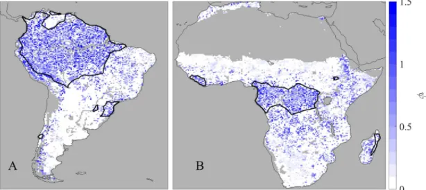
presence of first-order scattering in which the first-order scattering pathways (Fig. 3) become a significant contribution to radiometer measured TBp.Fig. 4displays the spatial distribution of estimated ω1in

South America and Africa. Non-zero values of ω1follow the spatially

coherent patterns of forests across both continents (e.g., Amazon Basin, Araucaria Moist Forests, Congo Basin, Guinean Forests of West Africa, etc.). Based on the dominant IGBP landcover classes in South America and Africa, forested pixels are predominantly characterized by the presence of first-order scattering contributions to the total emission. Specifically, 74% of forest pixels have non-zero ω1with a median value

of 0.06. Non-forest biome types in this region are predominantly characterized by an absence of first-order contributions. Specifically, 37% of lightly vegetated pixels (not including forests) have non-zero ω1

and accordingly the median ω1for pixels in each of these biomes is

zero. As one might expect, there is a tendency for taller vegetation to have higher ω1 though the correlation between variables is weak

(Pearson correlation coefficient between lidar height and ω1of 0.04,

p < 0.01).

ω retrievals from the zeroth and first-order implementations over

South America and Africa are shown inTable 1in comparison with available global empirical estimations and retrievals. The zeroth-order retrievals of ω are larger than empirically determined ω used in SMAP and SMOS baseline algorithms consistent with the SMOS-IC (Fernandez-Moran et al., 2017) and initial MT-DCA SMAP (Konings et al., 2017) ω retrievals. Since we have explicitly partitioned between single-scattering albedo and multiple-scattering effects, the results of increased ω in the first-order implementation with respect to ω in zeroth-order implementation are as one would expect, given theoretical single-scattering albedos are greater than effective scattering albedos (Ferrazzoli et al., 2002;Kurum, 2013). In other words, partitioning out the effects of multiple-scattering from ω in the proposed first-order RT model here results in retrieved ω closer to theoretical single-scattering albedos. The ω obtained from the zeroth-order implementation are in-herently lower as they effectively account for multiple-scattering. It is hypothesized that first-order scattering terms with closer representation to Kurum et al. (2011) terms would result in higher retrieved ω. Nonetheless, the addition of first-order scattering terms causes a ten-dency to increase ω estimations (see further discussion below and in Section 4.1).

ω1has a greater correspondence with lidar vegetation height when

normalized by ω (Pearson correlation coefficient of 0.39, p < 0.01), in a quantity we introduce here as ψ (ψ = ω1/ ω). ψ is shown inFig. 5and

assesses the ratio of first-order scattering magnitude to overall single-scattering properties within the homogenous medium. Due to evidence for a relationship with vegetation height and the representation of ω1

and ω, a higher ψ may be indicative of a denser vegetation structure present.

A non-zero ω1estimate suggests presence of first-order scattering

within the pixel and “activation” of first-order scattering terms in Eq. (6). We demonstrate that this also results in a better model-data fit between SMAP observed TBpand the first-order RT model than with the

zeroth-order RT model. Specifically, J1must be less than J0in order for

a non-zero ω1to be selected within the optimization. Here, J0is the

zeroth-order implementation cost function (where Eq.(11)is modified to minimize J1where ω1is zero; seeSection 2.3). For those pixels with

an estimated non-zero ω1, the median enhancement of model-data fit

(evaluated here as a percent reduction in residual: (J0− J1) / J1) is

typically small or about 2.5%. Since rp, γ, and ω appear in both zeroth

and first-order terms, it is unlikely that the first-order scattering terms act as free parameters to unphysically improve fit to TBpObs. Instead, we

postulate that the fit is improved due to the fact that the first-order terms are time-varying. While we acknowledge that ω1by itself can be

artificially adjusted in the optimization, the fact that ω1 magnitude

follows spatial patterns of forests inFig. 4suggests that this is largely capturing a physical phenomenon. Nonetheless, this does not mean that this improvement in model fit results in more reliable or accurate re-trievals.

ω1provides a quantitative basis to evaluate the first-order scattering

impact on radiometer measured TBp.Fig. 6displays the time averaged

TBH1stwhich typically ranges from 0 to 20 K with a median of 18 K (7%

of a given SMAP TBpmeasurement) for non-zero first-order emission

across all biomes. With ω1as a multiplicative factor of all first-order

scattering terms, it is no surprise that the spatial pattern compares closely withFig. 4. Since lightly vegetated biomes have a median ω1of

zero, their spatial median TBH1stis also zero. Thus, forest dominated

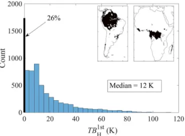
pixels greatly influence these estimates.Fig. 7displays the spatial his-togram of the time averaged first-order emission terms (TBH1st) for only

evergreen broadleaf forests in Africa and South America. 74% of forested pixels have non-zero first-order scattering with a median value of TBH1stequal to 12 K. This is 4.3% of a given SMAP TBpmeasurement.

This median percentage is determined from the time averaged ratio of

TBH1st to TBHTotalfor each forest pixel. Nearly identical values are

Fig. 4. Estimated ω1in South America (4A) and Africa (4B). Bold black outlines denote boundaries of evergreen broadleaf forests. Darker colored pixels suggest

greater first-order scattering which primarily occurs in regions with woody vegetation. Gray colored pixels represent no data due to static water body fraction > 5%, bare surface land cover, or land outside of the study region. (For interpretation of the references to color in this figure legend, the reader is referred to the web version of this article.)

Table 1

MT-DCA median effective ω estimates obtained here from zeroth and first-order implementations over South America and Africa compared with ω empirically determined for use in SMAP and SMOS baseline algorithms and estimated over the globe from SMOS-IC algorithm (Fernandez-Moran et al., 2017) and initial MT-DCA SMAP implementation (Konings et al., 2017). IGBP land cover classifications which comprise < 1% of the study region (Africa and South America) are not included due to low sample size.

Land cover classification SMAP baseline algorithm ω SMOS baseline algorithm ω SMOS-IC ω MT-DCA ω (Konings et al., 2017) MT-DCA0ω MT-DCA1ω

Evergreen needleleaf forest 0.05 0.06 or 0.08 0.06 0.09 – –

Evergreen broadleaf forest 0.05 0.06 or 0.08 0.06 0.09 0.08 0.11

Deciduous needleleaf forest 0.05 0.06 or 0.08 0.06 0.06 – –

Deciduous broadleaf forest 0.05 0.06 or 0.08 0.06 0.09 – –

Mixed forests 0.05 0.06 or 0.08 0.06 0.09 – – Closed shrublands 0.05 0.00 0.10 0.09 – – Open shrublands 0.05 0.00 0.08 0.08 0.10 0.13 Woody savannas 0.05 0.00 0.06 0.09 0.11 0.12 Savannas 0.08 0.00 0.10 0.08 0.10 0.12 Grasslands 0.05 0.00 0.10 0.08 0.11 0.19 Wetlands – 0.00 0.10 0.21 – – Croplands 0.05 0.00 0.12 0.11 0.14 0.19 Urban 0.03 0.00 0.10 0.12 – – Mosaic 0.07 0.00 0.12 0.11 0.11 0.16 Frozen 0.00 0.00 0.10 0.19 – – Bare 0.00 0.00 0.12 0.04 – –

obtained for vertical polarization (not shown). The median first-order emissivity is accordingly 0.04 which is less than the 0.15 to 0.25 first-order emissivity deciduous Paulownia trees determined inKurum et al. (2011). Figs. 6 and 7 provide quantitative evidence that multiple-scattering is contributing to the forest microwave signal at the SMAP radiometer footprint scale, information which could not be retrieved via implementation of the zeroth-order RT model with a constant ef-fective scattering albedo. Surprisingly, multiple-scattering appears to exist in pixels outside of evergreen broadleaf forests not flagged by SMAP as shown with 37% of pixels dominated by lightly vegetated regions exhibiting first-order scattering. The median TBH1stof these

pixels is 30 K. This can be attributed to the presence of large vegetation structures distributed amongst a pixel dominated by a lighter vegeta-tion cover.

SM and τ retrievals only change between zeroth-order and

first-order implementations when ω1 is non-zero. Therefore, white areas

(i.e., ω1= 0) inFig. 4have the same retrievals as with the zeroth-order

RT model in Eq.(1). This suggests negligible error in retrievals due to multiple-scattering if the zeroth-order RT model is used.Fig. 8shows

the difference in time averaged SM and τ retrievals between zeroth-order and first-zeroth-order implementations binned as a function of lidar vegetation height. Generally, accounting for first-order scattering in regions with taller vegetation (> 15 m) results in mean increases in both SM and τ on the order of 0.02 m3_/m3_{and 0.1, respectively. It is}

worth noting that SMAP baseline SM retrievals over core calibration/ validation sites have a dry bias on this order of magnitude though this may not be attributed to higher-order scattering as these sites are pri-marily lightly vegetated (Chan et al., 2016b). However, even if core calibration/validation in-situ forest sites existed, the “ground truth” provided by these measurements may be questionable with un-certainties in comparison statistics given spatial heterogeneity of SM and the presence of leaf litter.

Also, results inFig. 8suggest that Eq.(1)will result in negligible retrieval errors from multiple-scattering when lidar vegetation height is less than approximately 15 m at least in the case of SM. Vegetation between 5 m and 15 m should still exhibit presence of a scattering media. Based on the IGBP land cover classification, savannas and woody savannas correspond to the 5–15 m lidar vegetation height.

Fig. 5. ψ = ω1/ω in South America (5A) and Africa (5B). Bold black outlines denote boundaries of evergreen broadleaf forests. Darker colored pixels suggest greater

influence of first-order scattering magnitude with respect to single-scattering properties that takes place within the homogenous vegetation medium which primarily occurs in regions with woody vegetation. Gray colored pixels represent no data due to static water body fraction > 5%, bare surface land cover, or land outside of the study region. (For interpretation of the references to color in this figure legend, the reader is referred to the web version of this article.)

Fig. 6. Time averaged first-order scattering signal (TBH1st) over South America (6A) and Africa (6B). Bold black outlines denote boundaries of evergreen broadleaf

forests. These values are almost identical at vertical polarization and are not shown. Gray colored pixels represent no data due to static water body fraction > 5%, bare surface land cover, or land outside of the study region.

These regions are typically less dense than forests and are characterized by mixed clusters of trees and grassland. Therefore, it is possible that SMAP observed TBptypically (or 63% of the time) detects a mixture of

vegetation which does not produce significant volume, or first-order scattering effects.

4. Discussion

4.1. First-order scattering retrieval robustness

No other known study retrieved partitioned multiple-scattering parameters such as ω1from direct implementation of a higher-order RT

model at the satellite scale creating a challenge in comparing results. Over a deciduous Paulownia forest stand,Kurum et al. (2011)found first-order emissivity of approximately 0.15 to 0.25 which is larger than the median 0.04 emissivity determined here over tropical evergreen forests. This emissivity value was computed using effective physical temperature values noted inSection 2.4. Simulations of Eq.(6)under nominal conditions in forests determined first-order emissivities on the order of 0.1. Therefore, the approximate formulation of the first-order

RT model may inherently have a lower first-order emissivity than the-oretically developed first-order RT equations inKurum et al. (2011). This disconnect may be due in part to assumption (c) where first-order vegetation emission originates from the upper and lower canopy boundaries in Eq.(7)which can consequently overestimate fractional attenuation for each first-order scattering term. Additionally, differ-ences in satellite and tower radiometer footprints as well as tree types may prevent direct comparison between these results. The formulation presented here nevertheless likely provides an underestimate for the magnitude of first-order scattering at the SMAP radiometer scale. De-spite this, the magnitude of first-order scattering retrieved here can still significantly impact SM and τ retrievals as shown inFig. 8.

Since both zeroth and first-order RT models were applied within a retrieval algorithm, scattering properties can be compared. In areas where ω1retrievals are non-zero, the first-order implementation tended

to increase ω. While this positive relationship between ω and ω1could

result from their possible correlation within the first-order optimiza-tion, this phenomena is also physically expected since partitioning be-tween zeroth and first-order scattering terms should result in ω closer to theoretical single-scattering albedos which can exceed 0.5 for forests (Ferrazzoli et al., 2002). Since the zeroth-order implementation cali-brates an effective ω, it is including multiple-scattering effects which consequently reduces ω (Kurum, 2013). This gives some credence to our retrievals of scattering parameters in relation to theory. First-order implementation ω retrievals displayed inTable 1are still lower than theoretical single-scattering albedos, at least in the case of forests (which can be > 0.5). This is likely due to the first-order scattering terms in Eq. (7) having a lower emission magnitude than those in Kurum et al. (2011). Thus, improving correspondence between the simplified first-order RT terms in Eq.(7)and those developed inKurum et al. (2011)are expected to further increase both ω and ω1retrievals.

As expected, ω1and consequently first-order scattering are greatest

in the forested regions of South America and Africa. Additionally, ψ generally approaches and exceeds one in forested regions (seeFig. 5) suggesting that first-order scattering and single-scattering scattering properties within the homogenous vegetation medium are of similar importance. This approximated first-order RT model implemented within the MT-DCA is thus capturing at least the coarse scale upwelling emission that is scattered by the vegetation canopy. However, the ω1

estimated map inFig. 4and consequently derived figures that follow may be subject to noisy retrievals. Specifically, almost all primarily forested pixels should have at least non-zero ω1for all pixels, not only

74%. Conversely, one would expect that lightly vegetated biomes should almost all have zero ω1for all pixels, not only 63%. This is

within the context that scattering media which cause first-order

Fig. 7. Histogram of time averaged TBH1stover only forest-dominated pixels in

South America and Africa. 74% of forest-dominated pixels have a median TBH1st

of 12 K. The other 26% exhibit no first-order scattering at horizontal polar-ization. Insets show the location of evergreen broadleaf forests based on IGBP land cover classification. These values are almost identical at vertical polar-ization (not shown).

Fig. 8. Temporal mean difference between first and

zeroth-order SM (8A) and τ (8B) binned as a function of lidar vegetation height. Subscripts 0 and 1 represent zeroth and first-order implementation retrievals, respec-tively. All bins have an equal count of approximately 2500 pixels. The most predominant IGBP land cover classification for each bin is listed adjacent to each box in 8A and applies to 8B as well. Pixels dominated by sa-vanna and woody sasa-vanna have a zero median ω1

re-sulting in typically no change in SM and τ. Note that evergreen broadleaf forest is the dominant land cover for pixels in vegetation height bins > 17 m.

scattering (e.g., larger vegetation structures) are more prevalent in forests. Thus, these non-zero ω1in non-forested biomes may be due to

retrieval noise or the SMAP radiometer detecting large canopy struc-tures within the grassland/shrubland dominated pixels. The fact that the magnitude of ω1does not exhibit some finer scale spatial coherence

where adjacent pixels have relatively similar ω1values makes it likely

that non-zero ω1here is due to noise rather than a physical

phenom-enon (e.g., unexpected larger vegetation structures within a grassland pixel). However, the possibility of multiple-scattering in portions of biomes other than forests is still apparent as suggested by these results. We acknowledge some optimization instability of retrieving multiple parameters where correlations between retrieved ω1, ω, and τ are

pre-sent. This may be the case especially in forest-dominated pixels where a greater correlation between horizontally and vertically polarized TBp

measurements result in reduced DOI. However, an evergreen broadleaf forest pixel (located at latitude/longitude: 2.1°N/15.9°E) was tested for retrieval stability of ω1and ω adding mean noise under different

sce-narios from 0.1 K to 3.5 K to TBpmeasurements. It was determined that

even large amounts of noise (> 2 K) only changed ω1and ω retrievals

marginally (~0.01) thus exhibiting some robustness. Nonetheless, the fact that the majority of forested EASE-2 pixels yield a non-zero ω1

while less vegetated biomes are dominated by pixels with zero ω1

suggests that the first-order RT model and SMAP measurements exhibit some sensitivity to multiple-scattering from the dense vegetation structure. Retrievals within specific pixels should ultimately be inter-preted with caution.

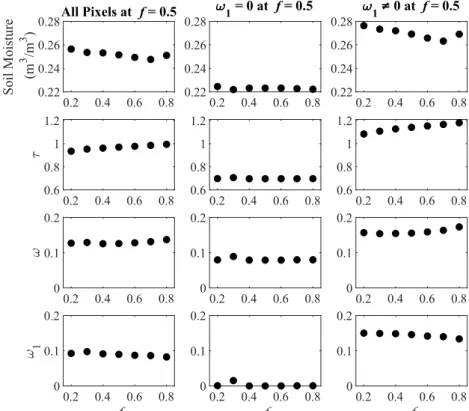
It is worth noting that retrievals are somewhat sensitive to the parameterization of f. 100 evergreen broadleaf forest pixels are eval-uated for their retrieval sensitivity to f varying f between 0.2 and 0.8 (where f is assumed to be a Dirac delta function at the first-order scattering centroid or concentrated at one height) as shown inFig. 9. In the cases when ω1is zero at f equal to 0.5 (where no first-order

scat-tering was detected in this study; 39% of the pixels in this region), it remained zero at other values of f with no corresponding changes in ω, mean τ, and mean SM. Thus, selection of f is unlikely to change whether or not first-order scattering is detected based on SMAP TBp

measurements. When ω1is non-zero at f equal to 0.5 (where first-order

scattering was detected in this study; 61% of the pixels in this region),

ω1, ω, mean τ, and mean SM vary, albeit marginally, when f is varied

between 0.2 and 0.8. Parameterization of f is thus a possible means to obtain a finer accuracy of the canopy representation, but may not alter the spatial pattern of retrieved variables.

Finally, the simultaneous retrieval of ω1and ω would not be

pos-sible without the polarization independence assumption. This assump-tion is relatively robust at a 40 km scale especially in forests due to random orientation of trees, but may break down under anisotropic alignment of vegetation (e.g., cropland).

4.2. Retrieval comparison with independent datasets

Retrieval comparisons with independent datasets are discussed where possible. SM retrievals were obtained using zeroth and first-order implementations on a 9 km EASE-2 grid using SMAP L1C TBpenhanced

product (Chaubell et al., 2016) over SMAP core calibration/validation sites listed inColliander (2017). However, these sites are located in croplands and grasslands which do not exhibit significant first-order scattering (< 40% of pixels with these land classifications are asso-ciated with a non-zero ω1 estimate). Specifically, a non-zero ω1

oc-curred in only 31% of cases with marginal changes in SM retrievals. Thus, SM in-situ comparisons are not discussed and forested in-situ sites would be required for more valuable comparisons. Additionally, other

SM in-situ measurement networks such as the Soil Climate Analysis

Network (SCAN) are too sparse to reliably compare with a 36 km re-solution SM retrieval.

No known in-situ VWC measurements over the temporal and spatial scale of the SMAP mission exist to compare with time varying τ. However, above ground biomass (AGB) estimates fromAvitabile et al. (2016)which combines the commonly usedBaccini et al. (2012)and Saatchi et al. (2011)estimates were gridded on 36 km EASE-2 grid and compared with τ retrievals from both zeroth and first-order plementations. Temporal mean τ from zeroth and first-order im-plementations were both highly correlated with AGB (Pearson's

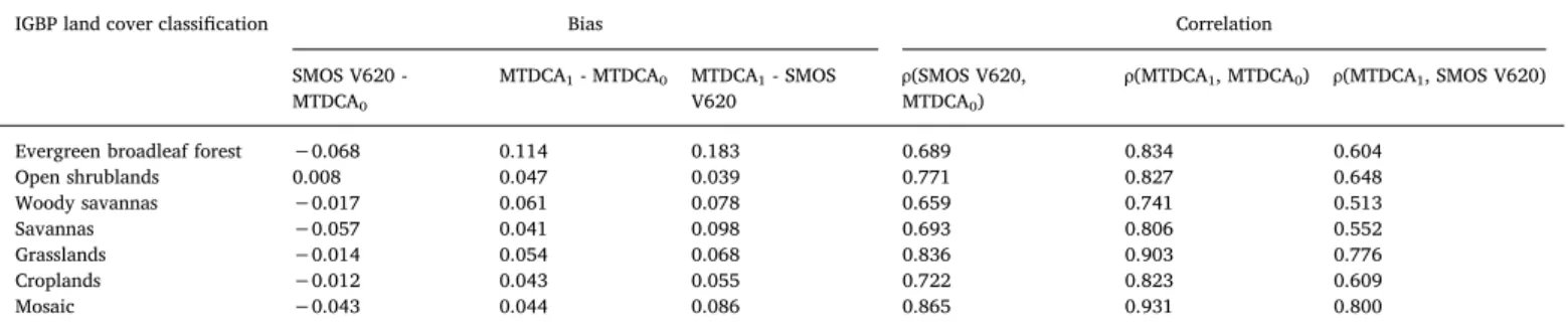
correlation coefficients of 0.87 and 0.85, respectively, p < 0.01) and lidar vegetation height (Pearson's correlation coefficients of 0.90 and 0.87, respectively, p < 0.01) across Africa and South America.Table 2 shows a comparison of time averaged τ retrievals between SMOS V620 product and MT-DCA zeroth and first-order implementations. Gen-erally, the MT-DCA first-order implementation τ is greatest and SMOS V620 τ is lowest. The higher mean τ biases between zeroth-order and first-order implementations in Table 2 is greater than what is re-presented inFig. 8B due to outliers contributing greatly to the mean bias. The spatial correlations are moderate to strong between all three datasets and strongest between MT-DCA zeroth and first-order im-plementations. The correlations are lowest between MT-DCA first-order retrieved and SMOS V620 τ especially in evergreen broadleaf forests, despite effective calibration of scattering over forest pixels in the SMOS L2 algorithm (Rahmoune et al., 2013). Similar τ temporal dynamics between zeroth-order SMAP MT-DCA and SMOS retrievals were es-tablished previously though they compare less closely for dense tropical forests (Konings et al., 2017). These two independent satellite radio-meters and algorithm retrieval approaches at L-band nevertheless provide similar estimates of τ.

ω retrievals do not necessarily have an independent equivalent

variable for comparison. However, values retrieved for the zeroth-order implementation here are comparable to initial SMAP and SMOS-IC re-trievals and generally higher than empirically determined values in the SMAP and SMOS baseline algorithms (Table 1). The fact that the first-order implementation ω retrievals are generally higher than the zeroth-order implementation ω retrievals is consistent with Kurum (2013) findings. This is because including first-order scattering terms partitions out multiple-scattering effects originally absorbed into the zeroth-order

retrieval of ω which is expected to increase ω closer to its single-scat-tering albedo definition. Estimates of first-order emissivity using ω1in

forests is 0.04, less than that determined byKurum et al. (2011)over a forest plot. Thus, the first-order scattering terms in Eq.(7)and thus ω and ω1may be underestimates of theoretically determined terms.

Without adequate validation, retrievals presented here should not be interpreted as enhancements to baseline SMAP and SMOS retrievals. This was not directly the goal of this study under the outlined research questions. A comprehensive forest monitoring campaign can create a basis for a reliable retrieval comparison. We hypothesize that the re-trievals may be more robust if this first-order RT model is implemented using SMOS TBp measurements as inputs due to simultaneous

mea-surements at multiple incidence angles. An additional basis for retrieval comparison is between the first-order RT model developed here and the two-stream RT model derived from MEMLS (Wiesmann and Mätzler, 1999) implemented recently for snowpacks (Naderpour et al., 2017; Schwank et al., 2015).

4.3. Effective scattering parameters and higher-order models

Fortunately, higher-order terms can be aggregated with zeroth-order RT terms in Eq.(1)to create effective parameters which account for multiple-scattering (Ferrazzoli et al., 2002; Kurum, 2013). This technique is currently in use in the SMOS V620 product over forests and is computationally efficient (Rahmoune et al., 2014, 2013; Vittucci et al., 2016). However, in this study, our purpose was to distinguish between areas where a transition between zeroth and first-order RT models may be important and consequently estimate the partitioned magnitude of first-order scattering. This requires a higher-order model

Table 2

Comparison of time averaged τ from SMOS V620, MT-DCA zeroth-order implementation, and MT-DCA first-order implementation over the study region. Bias and correlation statistics are computed spatially with all significant correlation coefficients (p < 0.05). There are > 1100 pixels for each IGBP class in each comparison. IGBP land cover classifications which comprise < 1% of the study region are not included due to low sample size.

IGBP land cover classification Bias Correlation

SMOS V620 -MTDCA0

MTDCA1- MTDCA0 MTDCA1- SMOS

V620 ρ(SMOS V620,MTDCA0)

ρ(MTDCA1, MTDCA0) ρ(MTDCA1, SMOS V620)

Evergreen broadleaf forest −0.068 0.114 0.183 0.689 0.834 0.604

Open shrublands 0.008 0.047 0.039 0.771 0.827 0.648 Woody savannas −0.017 0.061 0.078 0.659 0.741 0.513 Savannas −0.057 0.041 0.098 0.693 0.806 0.552 Grasslands −0.014 0.054 0.068 0.836 0.903 0.776 Croplands −0.012 0.043 0.055 0.722 0.823 0.609 Mosaic −0.043 0.044 0.086 0.865 0.931 0.800

Fig. 10. Comparison of emission behavior between zeroth and first-order RT models. A first-order model with ω1= 0.05 and ω = 0.12 (shown as solid curve) cannot

be accurately represented using a zeroth-order model (shown as dashed lines) with effective parameters. Other combinations of ω1and ω do not match zeroth-order

to contrast with the zeroth-order RT model. InFig. 10, we show that the functional form of the first-order RT model cannot be replicated simply by adjusting τ and ω in the zeroth-order RT model with a temporally constant ω in Eq.(1). This is because the first-order RT model explicitly represents approximated first-order scattering physics with the addition of first-order terms and factor, ω1. Due to additional computational load

in estimating ω1globally, it is conceivable that one could instead

esti-mate ω1and ω over in-situ sites with dense vegetation using Eq.(6)and

translate these values for global use in retrievals in forests in develop-ment of a SM product. This is left for future work and those attempting this or generally using Eq.(6)for SM retrievals are cautioned to all assumptions outlined in Section 2.2 in approximately representing multiple-scattering. Another approach for future retrieval investigation is a time-varying effective ω. This can be accomplished through esti-mation in the MT-DCA framework as suggested by Konings et al. (2017). Alternatively, a SM dependent time-varying ω can be computed using this first-order RT framework. The first-order RT model in this case can be simplified into the same form as the zeroth-order RT model as inKurum (2013)under the same assumptions for Eq.(7):

epTotal=(1 rp 2) (1+rp )(1 ) (12) e e e ( 2 ) (1 ) a b c 1 = + + (13) Maps and time-series of the time-varying effective scattering albedo may be produced using Eq.(13), but their inclusion is beyond the scope of this initial study.

A drawback of the proposed first-order RT model in Eq.(6)is the introduction of an effective rather than theoretical term, ω1. This

pre-vents direct comparison with parameters of other higher-order models, especially the “two-stream” RT model, MEMLS, developed inWiesmann and Mätzler (1999). However, investigations can be carried out in evaluating and comparing behavior of effective higher-order retrieved parameters with respect to other retrieved and ancillary parameters.

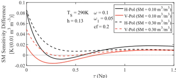
4.4. RT model sensitivity to soil moisture

If the proposed first-order RT model in Eq.(6)is used for SM or τ estimation, there is a potential benefit in increased SM sensitivity. The form of the zeroth and first-order RT models are compared here with respect to their sensitivity to SM. Since the first-order RT model in-cludes additional terms (i.e., first-order scattering terms) that contain more interactions with the surface (i.e., additional rpterms), we

pos-tulate here that this results in a greater sensitivity to SM under certain conditions. In order to comparatively evaluate the sensitivity of the zeroth and first-order RT models to SM, the SM sensitivity is computed for each model under nominal conditions through:

SM Sensitivity Difference TB SM TB SM p p 1st 0th = (14) where the subscript refers to the RT model order (i.e., subscript 1st uses Eq.(6)and 0th uses Eq.(1)). Simply, a more SM sensitive model is one that responds with a larger change in TBpmagnitude with a unit change

of SM. Each partial derivative is computed numerically by applying a ± 0.005 m3_/m3_{perturbation around a nominal SM value at nominal}

values of cf, TS, h, ω, ω1, and τ to determine the change in TBp.Fig. 11

plots the SM sensitivity difference by changing nominal values of τ under typical conditions for pixels in Africa and South America. This is repeated for two different values of SM (0.1 m3_/m3_{and 0.3 m}3_/m3_{) for}

both polarizations. Generally, the first-order RT model is more sensi-tive, albeit marginally, to SM at higher values of τ and SM which are typical conditions in the tropical forests in these study regions. This however may not necessarily result in improved SM retrievals.

The extra sensitivity to SM can be explained by the fact that the first-order terms in Eq.(7)include more interactions with the surface

(i.e., more emission terms with factor rp). This is quantified using

first-order implementation retrievals with a metric introduced here called the fractional surface contribution (in the case of f = 0.5):

Fractional urface Contribution T r e e r e

TB S [(1 p)(a b) 2 p c] p 1 s 2 1st = + + + (15) where the six first-order terms inFig. 3that include rpare normalized

by TBp1st. This is the fraction of first-order emission that interacts with

the rough soil surface. This is computed over each pixel with temporal mean values of rpand γ as displayed inFig. 12for horizontal

polar-ization (vertical polarpolar-ization is nearly identical and is not shown). Since any emission pathways that interact with the surface are largely atte-nuated in forests, the fractional surface contribution is inherently lower (~30 to 40%). However, this contribution is non-trivial and may pro-vide additional SM sensitivity. Also, since the first-order terms propro-vide extra surface interactions whenever first-order scattering is detected, it is unclear why SM sensitivity difference may decrease at low to mod-erate SM and τ values suggested byFig. 11. One can postulate that expanding to second-order RT terms in Eq.(7)would add extra surface interactions. However, this was not attempted as this is not practically possible due to computation load in iteratively solving the RT equations to the second order.

5. Summary and conclusions

In this study, our focus was to quantify the degree to which mul-tiple-scattering of microwave emission is important across a range of land cover classifications from grasslands to forests. This is ultimately of interest to those attempting to improve forest retrievals of SM at the satellite scale, a current challenge within the passive microwave remote sensing community due in part to the existence of multiple-scattering. In order to quantify higher-order scattering, a first-order RT model which explicitly partitions first-order scattering terms from zeroth-order emission terms was developed using a ray tracing method of single microwave interactions with the vegetation layer. It is an ap-proximated form of established first-order RT models which con-veniently includes the same variables as the zeroth-order RT model, commonly known as the tau-omega model. Though this introduces an additional variable, ω1which represents first-order microwave

inter-actions with the canopy, it provides an opportunity to retrieve parti-tioned single and multiple-scattering information across different biomes. We demonstrate that this RT model can be integrated within the MT-DCA framework to simultaneously retrieve time invariant ω and

ω1as well as time varying SM and τ without ancillary vegetation

in-formation. The algorithm was applied over Africa and South America,

0 0.5 1 1.5 (Np) -0.02 0 0.02 0.04 0.06 0.08 0.1 S M S en si tivit y D if fe rence [K /( 0 .0 1 m 3 m -3 )] H-Pol (SM = 0.10 m3/m3) V-Pol (SM = 0.10 m3/m3) H-Pol (SM = 0.30 m3/m3) V-Pol (SM = 0.30 m3/m3) T S = 290K h = 0.13 = 0.1 1 = 0.05 cf = 0.2

Fig. 11. SM sensitivity difference between zeroth and first-order RT models

with respect to τ. Vertical axis units are with respect to a 0.01 m3_/m3_{change in}

SM. Solid and dashed lines are SM sensitivity differences at SM = 0.1 m3_/m3

and SM = 0.3 m3_/m3_{, respectively. A SM sensitivity difference greater than zero}

means the first-order RT model is more sensitive to SM than the zeroth-order RT model. The dotted line is a reference for when the RT models have the same SM sensitivity.