The Character of Expiratory
Flow in the Lung
by
.John M. Co 11 ins
B.5., Rensselaer Polytechnic Institute
(1980)M.S., Massachusetts Institute of Technology
<1982)Submitted in Partial Fulfillment
of the Requirements for the
Degree of Doctor of Philosophy
in Mechanical Engineering
at the
Massachusetts Institute of Technology
January
21, 1988©
Massachusetts Institute of Technology,
1988Signature of Author
Certified by
Accepted by
Signature redacted
Signature redacted
' {
Roger
D.
Kamm
Thesis Supervisor
Signature redacted
Ain A. Sonin
Chairman, Department Graduate Committee
~HUIE
MAR 18 1988
The Character of Expiratory Flow in the Lung
by
John Mulloy Collins
Submitted to the Department of Mechanical engineering in January, 1988, in partial fulfillment of the requirements for
the degree of Doctor of Philosophy.
ABSTRACT
The primary objective of this study is to predict the expiratory pressure-flow relationship in a human lung.
Experiments and analysis of the flow in a single bifurcation provides a means to numerically synthesize the pressure-flow character for a complete lung, as well as providing insight
to the fluid dynamic character of expiratory flow.
A novel experimental technique was developed to measure the pressure drop across a single bifurcation within a multi-generation airway model. Energy considerations allowed the
pressure drop to be separated into components owing to kinetic energy fluxes and viscous energy dissipation.
Experiments were first conducted in an idealized symmetric, planar airway spanning the physiologically important Reynolds
number range from 50 to 8000. Sensitivity of the results was determined for typical pulmonary conditions;
- Non-planar geometries - L/D ratio variations
- Non-circular airway shape
- Asymmetric flow conditions
- Turbulent/Laminar flow regimes.
The numerical simulations of the human lung generated excellent agreement with available physiological data. Different morphometric models were investigated,
demonstrating the importance of the asymmetric geometry of the lung.
Thesis Supervisor: Dr. Roger D. Kamm
Table of Contents Page Abstract 2 Lift Vurr .f Fi 5 I. Introduction 1.1 Objective 1.2 Motivation 1.3 Approach II. Background 2.1 Forced Expiration 2.2 Flow Limitation 2.3 Work To-date III. Conceptual Framework
3.1 Bifurcation Flow Characteristics
3.2 Fully Developed Laminar Straight Tube F
3.3 Fully Developed Turbulent Pipe Flow 3.4 Steady Entrance Flow
3.5 Steady Flow in a Convergent 2-D Channel
3.6 Flow in a Curved Tube
3.7 Kinetic Energy Dissipation
3.8 Definition of Pressure Drop
3.9 Summary of Pressure Loss Correlations
IV. Experimental Methods
4.1 Subtraction Method
4.2 Downstream Boundary Conditions 4.3 Subtraction Method Analysis 4.4 Quasi-steady Test Apparatus
4.5 Experimental Scaling
4.6 Data Collection 4.7 Data Reduction
4.8 Technique Verification 4.9 Airway Models
V. Estimation of Correction Factors 5.1 Axial Velocity Profile Factor
5.2 Secondary Velocity Correction Factor
5.3 Pressure Correction
5.4 Correction Factor Implementation
11 16 23 low 52 78
Table of Contents
(Continued)
Page
VI. Symmetric Airway Results 93
6.1 Planar System Results
6.2 Embedded Bifurcation Assumption
6.3 Effect of Upstream Airway Orientation 6.4 Effect of Additional Parent Tube Length
6.5 Comparison of Results
6.6 Transition to Turbulence
6.7 Effect of Airway Collapse
VII. Flow Partition Experiments 113
7.1 Background
7.2 Experimental Procedure
7.3 Data Reduction 7.4 Results
VIII.Implications for Pulmonary Flows 125
8.1
Introduction8.2 Pressure Drop Correlations
8.3 Prediction of Model Experiments
8.4 Prediction of Physiological Model Experiments 8.5 Lung Simulations
8.6 Physiological Data
IX. Conclusions 148
References 151
List of Figures
Figure 1.3-1 Idealized dimensions of a pulmonary bifurcation, after Pedley (1971)
Figure 2.1-1 A typical maximal expiratory flow volume (MEFV) curve, and the effect of expiratory effort, after Bates et al (1971)
Figure 2.3-1 Comparison of published frictional pressure losses for the idealized bifurcation.
Figure 3.1-1 Typical four cell secondary flow pattern in the parent branch downstream of a bifurcation.
Figure 3.2-1 Velocity profile in a fully developed laminar tube flow, and the resulting force balance acting on a section of the tube.
Figure 3.3-1 Velocity profile in fully developed turbulent pipe flow.
Figure 3.4-1 Stepwise contracted tube pulmonary model, with constant L/D ratio's of 3.5, and area ratio's of 1.2.
Figure 3.5-1 Representation of laminar flow in a 2-Dimensional convergent channel.
Figure 3.5-2 Computed velocity profiles in a 2-D convergent channel flow for a range of flow conditions.
Figure 3.6-1 Secondary flow pattern in fully developed curved tube flow.
Figure 3.6-2 Generation of the four cell secondary flow pattern typical of expiratory flows from modeling a
bifurcation as two curved tubes oriented back to back.
Figure 3.6-3 Toroidal coordinate system used to analyze curved tube flow.
Figure 3.6-4 Prediction of the pressure loss in a curved tube, normalized by the Poiseuille loss at the same flow rate from the theory of Dean (1927).
Figure 3.6-5 Experimental results for the pressure loss in a curved tube, normalized by the Poiseuille loss that
would occur at the same flow rate, after Berger et al (1983)
Figure 3.9-1 Pressure loss correlations for curved tubes, entrance flow, 2-D convergent channel flow, and turbulent flows in straight and curved tubes.
Figure 4.1-1 Schematic representation of the subtraction method for symmetric flow conditions.
Figure 4.1-2 Pressure distributions owing to a 900 pipe bend between two long straight tube, after Ito (1960)
Figure 4.4-1 Schematic of the quasi-steady experimental test apparatus and pressure measurement locations.
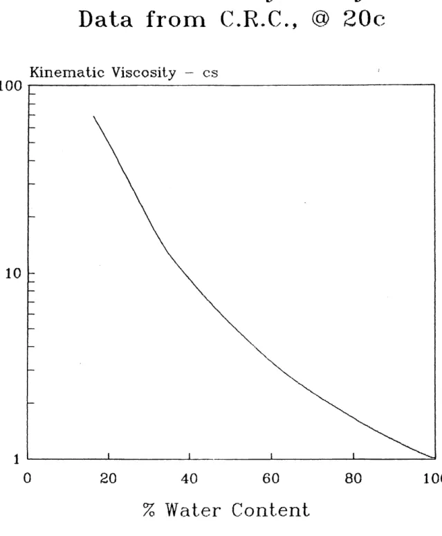
Figure 4.5-1 Kinematic viscosity of water-glycerin mixtures as a percentage of water content, from C.R.C.
Figure 4.6-1 Measured kinimatic viscosity for a 21% by
water glycerin-water mixture as a function of temperature
using Haake viscometer, and C.R.C. value.
Figure 4.6-2 Typical errors between tank level
calibration manometer readings and predicted levels based on the curve fits and output voltages.
Figure 4.8-1 Entrance test experimental bellmouth and straight tube geometry.
Figure 4.8-2 Tank level vs time measurements for the short entrance test (L/D = 6.3) at kinematic viscosities of
0.475 and 0.125 cm2/sec
Figure 4.8-3 Asymptotic region of the differential
pressure signal, showing a small offset error on the order of the digitation errors.
Figure 4.8-4 Error between the curve fit and the actual measured tank level, note that the magnitude of the error are
typically around the digitation level, and not systematic.
Figure 4.8-5 Calculated Reynolds numbers vs time for the short tube entrance test with kinematic viscosities of
0.125 and 0.475 cm2/sec.
Figure 4.8-6 Combined dimensionless pressure vs
Reynolds number for both entrance tests and the subtraction of the two, and theoretical predictions.
Figure 4.8-7 Results for the loss in the additional
length of tubing and theory.
Figure 4.9-1 Cross-section of a typical bifurcation showing the cast section and aluminum coupling collars.
Figure 5.1-1 Momentum analysis of an exiting jet impinging on a flat plat and turning 900.
Figure 5.1-2 Axial velocity profiles used to calculate the axial correction factor fa.
A)
Jan, Re=200 ;B) Chang & Menon, Re= 1060; C) Chang & Menon, Re=5712; D) Chang & Menon,Re=6000; E) Chang & Menon, Re=6811; F) Hardin & Yu, Re=2760; G) D.B. Reynolds, Re= 2260, Re=8000 and Re=12200
Figure 5.1-3 Cross plot of fa and a as calculated from the numerical integrals of published velocity profiles, and approximate relation.
Figure 5.1-4 - Results of the numerical integrals of fa
vs tracheal Reynolds number, and curve fit.
Figure 5.1-5 Approximate flow profile used to estimate the mean flow rate and fa factor based on boundary layer thickness.
Figure 5.1-6 Prediction of fa based on the boundary
layer approximation for an entrance prediction, at L/D=1.75
and 3.5, curved tube flow,
Sr=1/7,
and 2-D convergent channel flow, a=.05.Figure 5.2-1 Secondary velocity profiles used to numerically evaluate the secondary velocity correction factor, fs; A) Chang & Menon Re=1060,
@station
3, B)Chang & Menon Re=1060 @station 2s, C)Jan Re=200.Figure 5.3-1 Normalized pressure difference measured
between the top and side of bifurcation leg during expiration
vs local Reynolds number.
Figure 6.1-1 Experimental results for the reservoir level vs time for the experiments, Gen's 4-2, Nu=.475; Gen's 4-2, Nu=.125; Gen's 4-1, Nu=.475; Gen's 4-1, Nu=.125.
Figure 6.1-2 Subtraction of the three generation "upstream" airways from the four generation airway to give the normalized static pressure loss in the test bifurcation.
Figure 6.1-3 Decomposition of the total static
pressure loss across a bifurcation into a kinetic energy and frictional component normalized to '4P*Re2.
Figure 6.1-4 Frictional pressure loss across a single bifurcation normalized to the Poiseuille loss for the
symmetric flow experiments.
Figure 6.3-1 Configurations for the nonplanar symmetric flow experiments.
Figure 6.4-1 Subtraction of the three generation
"upstream" airways from the three generation airway with the additional tracheal length of L/D =3.5.
Figure 6.4-2 Frictional pressure loss in a straight tube, L/D =3.5, downstream of a bifurcation, normalized to the Poiseuille loss in the equivalent length of tubing.
Figure 6.5-1 Comparison of curved tube, entrance theory and 2-D convergent channel flow to the band of symmetric flow results.
Figure 6.6-1 Photographs of the oscilloscope traces from the hot wire probe, not transition to turbulence appears to occur near Re=1000.
Figure 6.7-1 Schematic representation of the bronchial support structure and pressure forces, after Hughes (1974)
Figure 6.7-2 Stereoscopic measurements of bronchial cross-sections at various transmural pressures, and two lung
inflations.
Figure 6.7-3 Normalized frictional loss in the semi-circular test bifurcation compared to curved tube theory
(note Reynolds number based on hydraulic diameter)
Figure 7.1-3 Most typical asymmetric bifurcation model in the middle airways, after Olson (1971)
Figure 7.2-1 Experimental apparatus for the flow partition experiments. Note separate fluid circuits.
Figure 7.3-1 Control volume selected to analyze the pressure loss in a bifurcation with asymmetric flow
conditions.
Figure 7.4-1 Results for the static pressure loss across the variable flow leg of a bifurcation, for six
different fixed flow rates in the other leg vs flow ratio, F.
Figure 7.4-2 Decomposition of the static pressure loss across a bifurcation into a kinetic energy component vs
tracheal Reynolds number. (fixed daughter Reynolds # of 1506)
Figure 7.4-3 Results for the excess pressure loss due to
the mixing of two streams vs F (flow ratio)
Figure 7.4-4 Momentum analysis of the maximum pressure recovery due to the unification of two unequal flows.
Figure 8.1-1 Comparison of the results for the friction pressure loss in an idealized bifurcation for this and
previous investigations.
Figure 8.2-1 Geometry of a typical asymmetric bifurcation used for analysis.
Figure 8.3-1 Comparison of numerical prediction, and experimental results of Hardin & YU, for the static pressure drop across an idealized three generation pulmonary model.
Figure 8.3-2 Comparison of numerical prediction, and experimental results of D.B Reynolds, for the static pressure drop across three generations of rigid "Y" connectors.
Figure 8.4-1 Depiction of the Zavala lung model, courtesy of Medi-tech, Watertown Ma.
Figure 8.4-2 Dichotomous branching pattern approximation for the Zavala lung model.
Figure
8.4-3
Comparison of numerical prediction, and experimental results of Isabey and Chang, for the static pressure drop across the Zavala lung model.Figure 8.4-4 Pressure drop components which comprise the calculated static pressure drop across the Zavala lung model for uniform pressure upstream boundary conditions.
Figure 8.4-5 Calculated Resistance matrix for the Zavala lung model.
Figure 8.4-6 A comparison of the flow distributions for the Zavala lung model.
Figure
8.4-7
Asymmetric branching pattern for the lung according to the Horsfeild et al (1971) lung Model 2.Figure 8.4-8 Comparison of numerical prediction, and experimental results of Reynolds and Lee, for the static pressure drop across a pulmonary cast below the right intermediate bronchus.
Figure
8.5-1
Comparison of the overall pressure-flow characteristics for the Weibel and Horsfield lung models.Figure
8.5-2
Pressure drop components which comprise the calculated static pressure drop across the Horsfield lungFigure 8.5-3 Percentage of "long" and "short" paths terminating at a given number of bifurcations into the lung.
Figure 8.5-4 Static pressure vs generation into the lung for both the Weibel and Horsfield lung models for several flow rates.
Figure 8.5-5 Normalized viscous pressure drop vs generation into the lung for both the Weibel and Horsfield
Figure 8.5-6 The variation of normalized viscous
pressure drop vs generation into the lung for Horsfield lung models for several flow rates.
Figure 8.5-7 Normalized viscous pressure drop vs average airway diameter for the Horsfield lung model at several flow rates.
Figure 8.5-8 Average and variation of the diameter and L/D ratio vs generations into the lung for both the Weibel and HOrsfiels lung models.
Figure 8.5-9 High and low Reynolds numbers Ratio factors vs generation for the horsfield et al lung model.
Figure
8.5-10
Comparison of the effect of flow types;inspiration, expiration and Poiseuille flows.
Figure 8.6-1 Comparison of the numerical prediction for pulmonary resistance based on the horsfield lung model and
the experiements of Blide et al, and Vincent et al.
Figure 8.6-2 Comparison of the numerical prediction for pulmonary resistance based on the horsfield lung model and
the experiements of Hyatt and Wilcox.
Figure 8.6-3 Comparison of the numerical prediction for pulmonary resistance based on the horsfield lung model and
1. Introduction
1.1 Objective
The primary objective of this work is to obtain a relationship between pressure drop and flow rate for expiratory flow from a human lung. Specifically, a
relationship is sought which describes the pressure drop across a single bifurcation which can be considered to be imbedded inside the airway network. A related objective is to gain
insight to the nature and character of expiratory pulmonary fluid dynamics.
The results of this study are intended to make it possible to synthesize the flow resistance of an entire airway system based on predictions for each of the individual bifurcations within the system. Accurate predictions require that the relationship be sufficiently general to allow for the
"non-ideal" characteristics of a real human lung. Pulmonary
parameters are known to change with position in the lung and with the evolving state of lung inflation during expiration. The number of potential combinations of these parameters which are encountered in the lung make it impractical to
experimentally investigate each one. A dimensional analysis of pulmonary flows to describe steady flow across a bifurcation
(Jaffrin and Kessic, 1972) identified the relevant
dimensionless groupings as the Reynolds number in each branch, and the geometric scaling parameters. This study will attempt only to establish a relationship for a typical bifurcation
within the lung over the of range Reynolds numbers in the
parent or tracheal branch from 100 to 10,000. The sensitivity of that relationship to the expected range of "non-ideal"
geometry and deviations from symmetry will also be examined.
1.2 MOTIVATION
The major motivation to study the expiratory pressure-flow relationship of a bifurcation is the desire to improve the diagnostic utility of the maximal expiratory flow volume
(MEFV) pulmonary function test. Computer models exist to predict the results of the MEFV as a diagnostic aid (Elad et al, 1987, Lambert et al, 1982), but these suffer from the lack of accurate pulmonary pressure-flow relationships.
The few correlations for expiratory flow resistance found in the literature (Reynolds, 1980, Reynolds and Lee, 1979, Reynolds, 1982, Hardin and Yu 1980) agree only to a factor of about three. While this variability could result from real
intra-study differences in the system geometry, the range is surprisingly large especially in view of the statistical
averaging that would result from multiple-generation networks. Further skepticism is based on the seemingly unrealistic limits approached by the correlations at both high and low Reynolds numbers.
A second, but equally compelling motivation to investigate the expiratory pressure-flow relationships is the profound lack of fundamental understanding of expiratory flows, even during
resistance exist (Pedley et al 1971, Pedley et al 1970a and b, Jaffrin and Kessic 1972), no equivalent extensive study of expiratory flow resistance has been conducted. Similarities are expected between inspiration and expiration, but
differences between the two flows, as discussed below, preclude a direct comparison.
1.3 Approach
The approach used in this study is primarily experimental. Analytical treatments of the problem are limited by the
complexity associated with a fully three dimensional flow
extending from low ('10) to moderately high ('10,000) Reynolds numbers. Some progress can be made, however, in the use of simple analogous flows. These are included to serve as both theoretical support for the results, and to aid in developing physical insight.
A novel experimental approach, called the subtraction
technique, was developed to provide the pressure difference across a bifurcation. This new method avoids the restrictive assumption made by most previous investigators that the form for the loss in a single bifurcation is the same for that found for the airway as a whole. It also avoids the substantial
errors involved in the direct measurement of the pressure drop across a single generation due to the considerable variation in pressure over the cross-section. A series of "companion"
experiments, including flow visualization and hot wire
turbulent flow.
Experiments were conducted on a network of bifurcations modeled after an "idealized bifurcation" presented by Pedley
(1977). The network from which casts were made was designed and fabricated in two pieces on a numerically controlled
milling machine by Drs J. Hammersley and D.E. Olson. (Univ. of Mich.) Figure 1.3-1 presents the dimensions of the idealized bronchial bifurcation, which can be further characterized as having;
w An ratio of the total daughter tube area to parent tube
area of about 1.2, based on a mean diameter ratio of .75
v A variable ratio of the radius of curvature of the tube center-line to the tube radius, with a mean of about
1/7. The tube curvature is greatest in the daughter tube at the bifurcation, and gradually straightens once the branching angle is reached.
a A changing cross-sectional shape which is circular in the parent and daughter tubes, blended with
progressively elliptical to dumbell shapes in the junction of the bifurcation.
a A branching angle, with a sharp flow divider, which varies from '640 in the large airways to 1000 in the smaller airways with a average value of about 700.
m Tube length/diameter ratio of 3.5 between bifurcations. x Smooth walls as a result of a thin mucas layer.
The idealized bifurcation was chosen rather than a cast from a real lung to maximize experimental control, and to
minimize the number of unknowns. Effort was directed first to understanding the most simple planar symmetric flow conditions and then extended to determine the sensitivity of the results to typical variations in upstream boundary conditions, flow
asymmetries and changes in bifurcation geometry.
Applicability of the results found in the constructed idealized models is investigated by comparing predicted and measured values of the pressure-flow relationships in rigid human lung casts.
2. Background
2.1 Forced Expiration
Despite the present lack of detailed understanding,
forced expiration has long been recognized as a valuable tool in assessing pulmonary function. Hutchinson (1846) recognized the technique as indicator of pulmonary vital capacity and pulmonary dysfunction over a century ago. It was not until the
insightful work of Hyatt et al, in 1958, however, that forced expiration results were described in the more useful form of maximum expiratory flow vs. lung inflation. Forced expiration
tests are currently used (Hyatt) to indicate the advent and progression of such important pulmonary disorders as:
a Emphysema v Bronchitis
v Cystic Fibrosis a Asthma
The utility of the MEFV function test is further enhanced because it can be generated from a relatively simple clinical evaluation (Hyatt 1983). The MEFV curves are generated from the flow vs. time traces obtained from a forced vital capacity, FVC, maneuver.
To obtain the FVC traces, a subject inhales maximally ( to total lung capacity ) and then exhales into a flow meter as forcefully and completely as possible to residual volume. The
total expired volume (total lung volume minus residual volume) is the expired lung vital capacity. Typically a Spirometer with an attached recording device is used to record the flow rate verses time. The FVC curves are integrated and
re-plotting as flow vs. expired lung volume to obtain the Maximal Expiratory Flow Volume (MEFV) forced expiration curve.
The MEFV curve, see Figure 2.1-1 (Hyatt, 1983), consists of two characteristic regions; one which is effort dependent and another which is effort independent. The effort dependent region occurs during the initial rapid increase in flow,
lasting until about 80% of vital capacity. The effort
independent region, or flow limited region, occurs with the decay in flow rate below approximately 75% of vital capacity. Curves corresponding to various degrees of effort are also shown in Figure 2.1-1, clearly demonstrating the effect of effort.
The utility of the MEFV curves in detecting pulmonary dysfunction is primarily a result of the flow limited portion
of expiration. During flow limitation for a given gas, the flow is only a function of the mechanical properties of the lung and the geometry of the lung.
2.2 Flow Limitation
The flow limiting nature of expiratory flow has been described by analogy to the flow limitation which occurs in thin walled collapsible tubes. Shapiro (1977a), in a summary of the physiological and medical aspects of flow in collapsible
tubes, describes the effect this way, " The (extremely
compliant) airways are easily collapsed by an in-wardly acting transmural pressure; the resulting decreased cross-sectional area makes for increased air speeds; this in turn produces an
increased pressure drop associated with the Bernoulli dynamic pressure and with frictional resistance"
Efforts to model forced expiration have proven extremely difficult because of the coupled effects of the airway
structure and fluid dynamics. Additionally, information on the mechanical properties of the airways and the detailed flow
behavior in a bifurcation is lacking.
To understand how these interactions and the effect of friction within the lung affects flow limitation, it is useful
to examine the equations for the thin-walled compliant tubes. A one dimensional model has been developed by Shapiro (1977b) to predict the structural/fluid dynamic interactions in a thin walled, massless straight compliant tube with varying wall
properties and rest area. The interactions are shown to depend on the following:
" The nature of the vessel structure in the form of
a " tube law " which describes the vessel area as a function of transmural pressure ( internal-external pressure ) and vessel stiffness, Kp.
" The external pressure acting on the vessel, and
both the end pressure boundary conditions.
" Frictional dissipation within the flow. " Changes in rest area along the vessel.
differential equation below; 2.2.1
dU -dAo d(P+gg2) 2S2f 1 dKp dp'
(1- 2) = - + + dx + - p' + Kp- dx
U Ao gC2 Dh C2 dx dx
where U is the mean flow speed, S is the ratio of U to C, the local tube wave speed, P is the static pressure, p' is the transmural pressure normalized to the the tube stiffness, Kp,
Ao is the local rest area, g is the fluid density, g is
gravitaional acceleration, Z is elevation, f is some friction factor which can depend on the local Reynolds number and
geometry, Dh is the hydraulic diameter defined as
4*area/perimeter, and x is the distance down the tube. Flow limitation occurs when the axial velocity of the fluid matches the local wave speed of the tube. When flow
limitation, or "choking" occurs, the flow will not be
increased by reductions in downstream pressure. This phenomena is exactally the same as that which is found in trans-sonic compressible gas flow and in the flow over a weir or "waterfall".
Much work remains before equation 2.2.1 can be applied with more confidence to expiratory flow. At best, only estimates can now be applied to each of the terms in the
equation. This work will concentrate
on
the frictional losses alone, and not attempt to describe the remaining terms.The effect of frictional dissipation on flow limitation can be seen from equation 2.2.1 to be unique. Friction which
toward a "choked" condition, increasing/decreasing the flow
speed to meet the local tube wave speed. For sub-critical
flows, S<1, the decrease in transmural pressure caused by
friction reduces the tube area, which, in turn, accelerates the flow toward the tube wave speed. In super-critical flows, the decrease in transmural pressure results in the opposite effect, a decrease in the flow speed toward the wave speed. It is
expected then that friction will play an important role in determining not only the required expiratory effort but also
the location of the flow limiting or "choked" point.
2.3 Work To-date
Relatively few studies have examined the frictional dissipation in an airway network during expiratory flow.
Pedley (1977) has made the the observation that "it is as if
everyone doing a model experiment on inspiration ran out of time or energy when it came time to repeating the measurements for expiration".
The few studies which are available consist mainly of
experimental model studies in airway networks which are either idealized planar geometric models or pulmonary cast models. Scherer (1972) developed a theoretical model to describe
expiratory flow through a single bifurcation. The assumptions required by Scherer's analysis, such as restricting the flow to a two dimensional form limits the utility of the model.
The comparison of available experimental studies (Reynolds
shows high variability in both the form and magnitude of results. Figure 2.3-1 graphically presents the inferred results for the frictional pressure loss in a standardized
bifurcation based on the correlations published for the results of the 4 different model studies. The standardized bifurcation chosen as the basis of comparison is a typical pulmonary
bifurcation as put forth by Pedley (1977), and graphically
depicted in Figure 1.3-1. The results for the pressure loss are normalized by the corresponding fully developed Poiseuille flow pressure loss through an equivalent length tube.
The magnitude of the results do not agree to better than within a factor of about 3. The nature of these results have
some puzzling attributes which appear to be inconsistent with intuition. First, at low Reynolds number the results are 1.5
to 3.5 higher than would be expected based on asymptotic limits
of fully developed Poiseuille flow. Second, with the exception of results of Hardin (1982), little similarity exists with the form of the pressure losses found in flows which are expected to be generally similar. These similarities tend to indicate that a Re'.5 dependence is likely to occur, and will be
discussed in more detail in the conceptual framework section. The inadequacy of these relationships is also seen when the pressure flow relationship found by D.B. Reynolds (1980) is
incorporated into expiration models (Elad et al 1985, Lambert & Wilson 1982). Elad et al (1985) found that the dependence of maximal flow on viscosity, especially at low lung volumes,
data from experiments conducted by Schilder et al (1963), Staats et al (1980), and Wood and Bryan (1969). The Lambert & Wilson model was able to produce a better viscosity dependence agreement with experiments, but required that the pressure losses be 3.5 times the corresponding laminar flow losses at very low Reynolds numbers.
A possible reason for these discrepancies may lie in the method used in previous studies for extracting local pressure-flow relations from global measurements. In all previous
experiments, the form of the pressure drop across a single bifurcation was assumed to be that found for the model as whole. Curve fitting was then used to determine the
coefficients for a single bifurcation. Imposition of this form for the relationship, which is actually a weighted average over the entire network, may mask the true form of the relation for a single bifurcation.
3. Conceptual Framework
3.1 Bifurcation Flow Characteristics
The complexity of the expiratory flow within a bifurcation is currently beyond the capabilities of theoretical analysis. The form of the Navier-Stokes equation which describes the flow cannot be solved analytically, and numerical treatments of the full three dimensional flow are beyond the practical limits of current computers. Current computational capabilities are
typified by the work of Wille (1984), which consumed about 2 months of processor time to solve the similar steady
inspiratory flow problem at a Reynolds number of only 10.
The remaining alternative to understand the flow is to use the results of model experiments in bifurcations to develop an understanding of the nature and character of the flow.
Similarities can then be drawn with the flow characteristics in similar, but less complicated flows. Generally, the less complicated flows are better understood, and the proper
analogies taken together can form a conceptual framework in which to interpret expiratory flows.
Flow visualization and hot-wire velocity mapping studies performed in airway models and in single bifurcations (West and Hugh-Jones 1959, Schroter and Sudlow 1969, Patra and Afify
1983, Chang and Menon 1985, Jan 1986 ) have lead to a number
of consistent observations on expiratory flows;
a The most notable is that a four cell secondary flow pattern occurs downstream of the junction for tracheal
Reynolds numbers from 50 to several thousand. This flow pattern is shown schematically in Figure 3.1-1.
a The secondary flow pattern is developed either within
the junction or just downstream of it.
a Flow patterns are qualitatively similar for the range of
inlet conditions tested; fully developed parabolic inlet flows, blunt inlet flows, and flows with secondary flows similar to those found in the outlet.
a The magnitude of the secondary flow velocity is between
approximately 1/5 and 1/2 of that in the bulk axial flow.
n Axial velocity profiles just downstream of the junction
contain a dip which is rapidly transformed into a peak in the plane of the bifurcation, but remains flat in the plane normal to the bifurcation.
m Distances greater than about one diameter downstream of
the junction, the axial velocities are "blunt", and are
characterized by a relatively thin boundary layer.
a For the case of a long straight parent branch, the
secondary flows generated in the bifurcation are convected downstream through the equivalent of many branch lengths.
Inspection of these flow characteristics, and the geometry of a bifurcation lead to the consideration of several flow
types as possible analogies to steady expiratory flow. The following are the flow problems for which possible analogies
apply, and are well understood based on experimental and theoretical investigations.
a Fully developed steady laminar flow in a straight tube. a Fully developed steady turbulent flow in a straight
tube.
a Steady entry flow in a straight tube. a Steady flow in a convergent 2-D channel.
s Fully developed steady flow in a curved tube.
3.2 Fully Developed Laminar Straight Tube Flow
Fully developed straight tube flow was one of the earliest analogies drawn to describe pulmonary flows (Rohrer 1915). The analogy stems from geometric similarities given that airways, in the most elementary form, can be considered a
series of straight tubes. The analogy neglects the effects of curvature on the secondary flows and that each tube section is typically too short for a fully.developed flow to develop. Schlichting (1979) gives the entrance length required to
establish a fully developed Poiseuille profile to be;
3.2.1 Le=0.03*Re*Dia
A fully developed flow will therefore not evolve within a bifurcation which has a typical length of 3.5*Dia. (Pedley
1977) until the Reynolds number drops below about 100. For
Reynolds numbers significantly below 100, though, an increasing length of the tube will be fully developed. The frictional dissipation in a fully developed straight tube flow therefore serves as a low asymptotic limit for the flow in a bifurcation.
Derivation of the fully developed pipe flow equations can be found in most text books
on
fluid mechanics. The problem represents the Navier-Stokes equation in its most simple form;dP du2
3.2.2 - =
-dx dr 2
axial position, p the pressure, and p is the fluid viscosity.
Solving 3.2.2 for the pressure drop across a tube of
length L gives;
3.2.3 Del P = 32pLU/D2
where U is the bulk averaged velocity defined as the flow rate divided by area, and D is the tube diameter. Equation 3.2.3 can be written in another form which introduces a
characteristic pressure P*, and the Reynolds number
3.2.4 Del P =32 L/D P* Re
where p* is given by;
* y 2 ;Nu
2
3.2.5 P = =
gD2 D2
where Nu is the kinematic viscosity.
A scaling argument which provides more insight to the nature of the pressure drop can be used to arrive at the same result to within a constant factor. While this is not
necessary due to the susceptibility of the problem to rigorous analysis, it helps to establish a comparison for other more complicated effects.
From a force balance on a section of tube with a length L, shown in Figure 3.2-1, the pressure force acting on the tube cross-sectional area, can be seen to be balanced by the wall shear stress acting on the wall;
3.2.6 (P1-P2)nD2 = TW(rDL)
where
Tw
is the wall shear stress, and for a Newtonian fluid is given by;du
3.2.7 Tw =
A-dr wall
which can be approximated by representing the velocity gradient at the wall as the ratio of a characteristic
velocity, the bulk velocity, by a characteristic length, the tube diameter. Combining the approximation with equations
3.2.7 and 3.2.6 gives the pressure drop as;
3.2.8 Del P =P - P = Const.*PLU/D2 1 2
Comparing equation 3.2.8 and 3.2.3 shows that the two
forms agree if the unknown constant in equation 3.2.8 is taken to be 32.
3.3 Fully Developed Turbulent Pipe Flow
Laminar flow in a smooth straight tube will remain despite the presence of slight vibrations and other perturbations
encountered in "real world flows" for as long as the flow is stable. Instabilities occur in steady flows when the inertial effects dominate the viscous effects. Stability is typically characterized by the ratio of these two effects in the form of
the Reynolds number. A Reynolds number near 2300 for steady pipe flows is the value at which the flow becomes unstable, and therefore subject to turbulence.
Turbulent flows are expected to exist in expiration both because of the high Reynolds numbers encountered, and the significant flow disturbances which are present. As will be discussed later, the conditions for transition are complicated
by spatial accelerations and secondary flows, both of which are
expected to delay transition to higher Reynolds numbers. No theory based on first principles is yet available to describe turbulent flows, and, the small scale of turbulence renders computer models impractical for a complete solution of all but the simplest of flows. Experimental results have, though, lead to a detailed understanding of structure of turbulence.
The pressure loss in turbulent smooth-walled pipe flows has been well documented (Schlichting 1979), and can be explained with the scaling arguments outlined above for laminar flows. Referring to Figure 3.3-1, unlike laminar flows, turbulent flows are characterized by a relatively blunt velocity profile with a thin boundary layer. The small scale eddies efficiently
transfer momentum radially to smooth the velocity in the core. Imposition of a no-slip boundary at the wall, generates a
region of laminar flow with high shear close to the wall. Estimation of the shear stress in the laminar sublayer which acts on the wall is then given by;
du u(S)
3.3.1 -w = )4 - 0
dr wall 8
velocity at the boundary layer edge, and are given by;
3.3.2 8 a P/v*
3.3.3 u(S) a V*
where v* is the characteristic velocity for turbulent flows;
3.3.4 v * / ( (Tw / g)
Experimental measurements of velocity distributions and wall (see Schlichting) shear stress give v* to be;
3.3.5 v* = .1823
[U
/r 1/8combining 3.2.4 and 3.3.1-3.3.5 gives the familiar Blasius friction relation for smooth walled turbulent pipe flows;
'4
3.3.6 Del P = 0.3146(4gU2)(L/D)/Re
where Re is the tube Reynolds number Re = Up/gD. Using the p* notation, equation 3.3.6 can be written more concisely as;
* 1.75
3.3.7 Del P = 0.157 P (L/D) Re
For the case where surface roughness extends into the flow past the laminar sublayer, this relation no longer holds. A
transitional region exists when the mean roughness height, Ks, is between the laminar sublayer , yv*/nu=5 to about yv*/nu =70. For Ks above yv*/nu=70 the flow is considered fully rough, and the increased velocity gradient at the wall generates the
pressure drop given by the expression;
3.3.8 Del P= '4P L/D Re2 2Log(r/Ks) + 1.74
Schroter and Sudlow (1969) have noted that bronchial walls are coated with a liquid mucus layer which is "microsopically"
thin, and therfore hydraulically smooth. Macroscopic
corrugations in the trachea and main bronchi are present due to cartilidge rings. The effective Ks generated by these
corrugations is relatively low due to their wide spacing. These corrugations are therefore unlikely to generate fully
rough flow. Consequently it is more probable that 3.3.7 will apply in the lung, rather than 3.3.8.
3.4 Steady Entrance Flow
The entrance type phenomena expected in a bifurcation are similar to those for the steady entrance flow problem in a straight tube, but more complicated. The entrance phenomena are a result of the effects of viscosity diffusing in-ward from the wall to adjust the inlet velocity profile to its fully
developed final form. The extent of the difference between the inlet profile and the fully developed profile will therefore determine the magnitude of entrance effects on the flow.
The entrance analogy in expiratory flows can be seen by considering a lung as being roughly modelled by the geometry
flow proceeds toward the "trachea" can be approximated as a series of straight tube sections, L/D = 3.5, with a constant
area ratio contraction, An/An+1=1.2, joining the tubes. The viscous effects start to propagate in from the wall as the flow proceeds in each straight section. In the contraction section, the flow accelerates, and the viscous boundary layer thins to maintain continuity. Once in the straight section, the boundary layer continues to grow, but starts from a non-zero value.
Rivas and Shapiro (1956) in an analysis of ASME test nozzles accounted for the non-zero initial boundary layer thickness in the straight tube section downstream of a
bellmouth entrance with an "equivalent length" concept. The equivalent length, Leq, is the length of straight tubing required to develop a boundary layer thickness equivalent to
that found in the inlet of the straight section downstream of the bellmouth. In general, the equivalent length is dependent on the flow rate, and bellmouth geometry. The loss downstream of the entrance can then be calculated as the difference in a
tube of the actual length plus Leq, and a tube of length Leq. Applying entrance flow theory with the added correction of an equivalent length to expiratory flow is difficult. The difficulty arises due to the presence of secondary flows, nonuniform inlet velocity profiles, and the flow details required to calculate Leq. Despite these problems, entrance
flow analogies have been applied with some success (Pedley
provide some understanding of expiratory flows.
A sizeable amount of literature has been devoted to the study of flow in the entrance of a circular pipe. Boussinesq
is the first to be cited as having made a theoretical
investigation of the problem in 1891. Since that time many experimental studies have been done, and correspond well to
theoretical predictions. Most current analyses of the problem are numerical, but the more simple boundary layer analysis of Boussinesq provides insight to the flow character for large Reynolds numbers.
Investigations (Shapiro et al 1954) have shown that for the thin boundary layers near the entrance, the falling
pressure gradient has negligible effect on the boundary layer development. Flat plate, Blasius type, boundary layer growth therefore occurs, which gives the boundary layer thickness as;
3.4.1 S(x)=1.72DV(x/DRe)
where D is the tube diameter, x the distance along the tube axis, and Re is the tube Reynolds number. In the first
approximation, the core velocity can be taken to be constant, which allows the wall shear rate to be written as;
du U Re
3.4.2 Tw(x) = - - = JU
dr wall S(x) xD
A2 R3 4 3.4.3 Del P const. Re L/D
where the published experiments place the constant as 4.87. Note that the typically reported value is 6.87, which is higher because it includes the effects of the changing velocity
profile. Incorporating the equivalent entrance length and P* into equation 3.4.3 gives;
3.4.4 Del P = 4.87 P *
[
(L/D + Leq/D) - Leq/D] Re The validity of this expression for straight tubes isconfined to intermediate values of Reynolds number. On the low end of the range, the thin boundary layer approximation fails as the entrance length approaches the tube length, and
Poiseuille flow results. For cases in which the product of the Reynolds number and L/D ratio exceeds about 10E5, turbulence is present in the boundary layer and the growth pattern of the boundary layer is altered.
This boundary layer transition to turbulence may arise in expiratory flows. Assuming an Leq near 1, with an L/D ratio
of 3.5, the transition would occur on the order Re'10,000.
3.5 Steady flow in a convergent 2-D channel.
Another geometry that can be used to model both a single bifurcation and the entire airway is a convergent channel. This representation is not very accurate, but provides a means
boundary layer growth and thinning. The growth of the boundary layer results from the diffusion of viscosity as the fluid
passes through the network, while the boundary layer thinning results from the increasing velocities imposed by the
progessively smaller flow area.
Schlichting (1979) has summarized the exact solution to Navier-Stokes equation for the 2-D channel. The equations can be considerably simplified for this case in which the flow is everywhere radial, and the flow profile depends only on the azimuthal angle, 0. The geometry is shown in Figure 3.5-1. Defining a local Reynolds number as;
Uo h
3.5.1 Re =
Nu
where Uo is the local centerline velocity, and h is the local channel height. Normalizing the velocity by Uo, and the radial distance by h, allows the N-S equations to be written in terms of a single non-linear differential equation;
Re 2 62u- -K 2a
3.5.2 -- + 4 U +
2o 802 Re
with the boundary condition;
3.5.3 G( a ) = 0 .... No slip at the walls.
3.5.4 S&( 0 )
= 0 ... Centerline symmetry
with the definitions;
-1
3.5.6 a = Tan ( '4h/r ) z
uh/r
The convergence angle, a, which is appropriate for use in the lung is difficult to define because of the difficulty in converting from a three-dimensional to a two-dimensional
geometry. One approach to define an appropriate value of
a
for the lung is to write the area of the lung in the exponential form;3.5.7 A = A exp
[0-=
L
]
which can be linearized about a typical bifurcation with an L/D of 3.5 and an area ratio of 1.2, giving o as approximately
0.052 (representing an included divergence angle of about 60).
The constant K in equation 3.5.2 is the imposed wall pressure gradient, in the form;
3
r SP
3.5.8 K =
-g Nu2 Sr wall
Equation 3.5.2 can be solved numerically, or analytically for the extremes in Reynolds numbers. The numerical solution to 3.5.2 is presented in Figure 3.5-2 for the dimensionless velocity profile for a range of Reynolds numbers and the
typical pulmonary value of a. The profile is seen to progress from a Poiseuille type profile at low Reynolds numbers to a profile characterized by a blunt core and thin boundary layer at higher Reynolds numbers.
follow the same progression from a Poiseuille form to a
boundary layer form. The boundary layer form can be seen most easily by solving 3.5.2 for the high Reynolds number case and evaluating the wall friction. The high Reynolds number limit solution to 3.5.2 is;
-1
3.5.9 u = 3Tanh2 (Re a/2) (1 - O/a) + Tanh V(2/3)
which generates a shear stress at the wall corresponding to the pressure drop;
Del P 2
3.5.10 = a cos( a Re
0(O)
Del P -/3 L
pois.
Using the value a = 0.052, corresponding to the lung, and
numerically evaluating 0(O) to be approximately 1.15, gives the asymptotic frictional relationship to be;
3.5.11 Del P Z Del P .06 -/Re Re
>>
1A relationship which can be applied to lower Reynolds numbers must be obtained from the direct solution to 3.5.2.
3.6 Flow in a Curved Tube
The generation of secondary flows downstream of a
bifurcation during expiration can also be described by analogy to curved tube flow. Figure 3.6-1 shows the secondary flow
pattern established by the centrifugal forces generated by the core flow as the flow proceeds around the bend in a curved tube. The resulting pressure gradient across the tube cross-section causes fluid in the core to move outward where the slowing moving fluid at the wall has insufficient axial
velocity to generate the same pressure gradient, and is driven inward to preserve continuity.
The four cell structure found in the parent tube of a bifurcation, shown in Figure 3.1-1, can be generated by approximating the bifurcation geometry as two curved tubes oriented back to back. This geometry is depicted in Figure
3.6-2, and shows that for symmetric flows a balanced four cell
pattern is expected.
A basic difference which must be noted between curved tube and flow in a bifurcation is that in a bifurcation both the geometry and area change as the flow proceeds along the bend. Despite these differences the analysis of the driving factors which influence curved tube flow should provide insight as to
the nature of secondary flows in expiratory flow. This hypothesis is supported by the -work of Jan (1986) which
indicated similarities between the velocity profiles in quasi-steady oscillatory flow in a bifurcation those predicted with curved tube flow theory.
For curved tube flow the natural coordinate system is a toroidal one, as shown in Figure 3.6-3. The orthogonal unit vectors are in the r,
a,
and s directions where r is measured radially outward from the center of the cross-section,a
is theangle between the radius vector and the plane of symetery, and s is measured along the tube axis. In this coordinate system the steady non-dimensional Navier-Stokes equation take the form given in Equation 12 of Berger et al. The dimensional
parameters ( denoted with a ') are nondimensionalized by;
r = r'/a s = RcO/a p = p'/(gU2)
3.6.1
u = u'/U v = v'/U w = w'/U
Berger, Talbot and Yao (1983) outlined a simplification of these equations for the case of gradual curvature, Sr = r/Rc
<<
1, by neglecting all terms of order Sr' or higher. Thecentrifugal force terms which are necessary to drive the secondary motions were retained in the analysis by rescaling the axial velocity as;
3.6.2 u = u'/ [Udr I
and for convenience the axial distance is rescaled as
3.6.3 z = sr
Introducing the Dean number, Dn, which is the ratio of the square root of the inertia and centrifugal force product to the viscous force;
'4 3.6.4 Dn = Re Sr
the resulting equation, along with the continuity condition for fully developed flow is given in equation 13 of Berger et al. This equation was obtained by recognizing that the velocities
no longer vary with axial position. Inspection of this
equation indicates that the axial pressure gradient is linear. A stream function is introduced and, following
cross-differentiation to eliminate the pressure, equations 15 and 16 of Berger et al are obtained.
For small values of Dn the equations can be solved by expanding the solution in powers of Dn about the Poiseuille straight tube profile. The result, when expressed in terms of the axial pressure difference is given by Dean ( 1927,1928);
Del P 2 4
3.6.5
[
1 +.0306(K/576) -. 0110(K/576) + .Del Ppois.J
where Del Ppois. is the the Poiseuille pressure drop in a straight tube with the same flow rate, and K is the original form of the Dean number defined by Dean as;
a Wmax a 2
3.6.6
KE=
[
Rc L Nu2
where Wmax is the maximum velocity in a straight pipe of the same radius resulting from the same imposed pressure gradient. The relationship between Dn and K depends on the ratio of the flux in the straight tube at a specified pressure gradient, Qs, and the flux in the curved tube with the same imposed pressure gradient, Qc;
Qs '
3.6.7 Dn - E'/ K]
where the ratio Qc/Qs,is (Berger et al);
Qs 2 4 6
3.6.8 - = 1 -. 0306(K/576) +.0120(K/576) + O(K/576) Qc
Dean's series expansion solution is valid up to Kz576. Figure 3.6-4 presents the results of deans solution for the pressure loss in a curved tube normalized to that in a
Poiseuille flow with the same bulk flow rate verses Dn. The graph was generated by calculating the flow ratio based on a
value of K, and then the finding the Dn corresponding to K and the flow ratio. It is interesting to note that for Dn S 10, effects of curvature on the pressure gradient are almost
negligible. Even at the high limit of applicability for Dean's solution, the effects are small, generating only a 2% increase
in the flow resistance at K=576, corresponding to Dn-16.
The nature of the flow and the scaling of Dean's solution for the secondary flow can be understood by considering the forces acting on the fluid. The axial velocity establishes a pressure gradient which is balanced by the shear stress at the wall induced by the secondary flows. The resulting pressure
balance can be written as;
2
g;U Vsec
3.6.9 r - ^
Rc r
which gives the secondary velocity scaling found by Dean; Vsec
3.6.10 Sr Re
At higher values of Dean number, numerical studies have been utilized to solve equation 3.6.7. The most expansive of these numerical studies is by Collins and Dennis (1975) who were able to extend Dean's solution up to Dn=5000. The numerical studies suggest that the structure of the curved tube flow at high Dean numbers is that of an inviscid
rotational core surrounded by a thin boundary layer at the tube wall.
An understanding of the nature and flow characteristics which typify the high Dean number curved tube flow can be
gained by investigating the asymptotic limits of the governing equations. Pedley (1980) formed the asymptotic limits by
scaling equation 3.6.7 with the asymptotic form for the streamfunction, 0, Dean number, Dn, and boundary layer thickness, S;
3.6.11a Dn U /K
a
3.6.11b ' -1K /Dn
3.6.11c S K
Note; Pedley used a dean number, D, defined as
/K,
and normalized velocities by Nu/a rather than U. These differences in notation account for in the somewhat unusual notation presented in 3.6.14 to preserve the form of Pedley's analysis.For the core flow, the viscous effects are negligible, and the pressure gradient established by the centrifugal forces
are balanced by the inertial terms: equation 3.6.7a therefore gives;
1
= a + a
In the boundary layer, there is a balance between the inertia, viscous and the centrifugal force terms gives;
4T + a - 2a = 2(a - a) + 3T = T
Solving the three equations for the three unknowns gives;
a = T = *'a = 1/3
which can be inverted to give the parameters in terms of Dn;
3.6.15a 3.6. 15b 3.6.15c 1/cJ /K ' Dn 1.5 = Dn S 1/K /Dn = Dn 8 /K = Dn
The pressure drop is therefore seen to go as;
L L du Del P = Tw - = P - -D D dr wall U L 8 D *L SP - U Dn D
In contrast to the secondary velocity scaling at low Dean numbers, equation 3.6.15 allows the secondary velocity scaling to be written directly as;
3.6.12
3.6.13
3.6.14
U U Dn
3.6.17 Vsec U
Dn
giving the ratio of secondary velocity to that in the core as a constant, unlike the low dean case in which the ratio
increases with Dean number.
These asymptotic forms have been verified by numerous experimental and numerical studies and are summarized by
Berger et al (1983). Results of the experimental studies for the frictional losses are shown in Figure 3.6-5. The
experimental data is sden to be correlated well by the Hasson correlation below curvature dependent branch points which are identified as transitions to turbulence. The correlation is valid down to a Dn of about 20 where Dean's solution asymptote
to Poiseuille flow. The Hasson correlation is;
*L r
3.6.18 Del P = 32 P - Re 0.556 + 0.0969 Dn
D LJ
Ito (1959), experimentally documented the frictional loss in turbulent flows for a curved tube. The transition to
turbulence was found to be retarded by the action of the secondary flows. The exact reason for the postponement of transition is still not clear, but it is generally believed that the action of secondary flows to thin the boundary layer
is similar to the effect of a favorable pressure gradient. For the range of experiments 1/15 > Sr > 1/9000, Ito reports the critical Reynolds number to be;
0.32
3.6.19 (Re)crit = 2E4 Sr
The experiments were correlated by a Blasius type expression with an additional curvature effect;
* L r-3/8 -'4 2
3.6.20 Del P = 4 P - Sr 0.029 + 0.034 Sr Dn Re D L
validated over the experimental range;
1.5
300 > Dn Sr = Re Sr 2
> .034
1.5
For larger values of Dn Sr , the expression becomes;
1/5
L Sr 2
3.6.21 Del P = ' P - 0.316 Re
D Dn
While the typical curvature encountered in the lung, '1/7, is below the range of Ito's experiments, it can be used to estimate a critical reynolds number of about 10,000. This places the Re Sr2 product at 200 at transition, indicating that 3.6.20 is the most likely form applicable to pulmonary conditions.
3.7 Kinetic Energy Dissipation
The case of expiratory flow through a bifurcation which is embedded within an airway can be considered fully developed in the sense that the entering velocity profile will be similar to
the exiting velocity profile. This must be the case for a fully developed symmetric flow within a "large" airway system because the inlet of a bifurcation will be the outlet of
another bifurcation.
The most striking feature of this situation is that a total of eight vortices in the two inlet flows are converted within the bifurcation to only four in the outlet. The
mechanism for this conversion is not clear, although it can most likely be considered to fall between two extreme
alternatives:
a Each of the eight inlet vortices are dissipated
through viscous action, and four more are
generated through the conversion of potential to kinetic energy.
n The kinetic energy of the inlet vortices are
conserved by the enhancement of the two outer vortices of each daughter tube by the two inner vortices feeding them through the secondary flow.
The dissipation in the first case would be similar in nature to fully rough turbulent flows in which large eddies are generated and then dissipated due to viscous action. The generation and dissipation of the secondary flow vorticies will not occur randomly as in turbulent flow, but will occur once at each bifurcation. Another difference from turbulent flow is the orientation of the secondary velocities. In bifurcations, the vorticies are oriented along the axis of flow, which is not always the situation in turbulent flows
(Schlichting, 1979).