Calibration of the Demand Simulator in a
Dynamic Traffic Assignment System
by
Ramachandran Balakrishna
B.Tech in Civil Engineering (1999)
Indian Institute of Technology, Madras, India
Submitted to the Department of Civil and Environmental Engineering
in partial fulfillment of the requirements for the degree of
Master of Science in Transportation Systems
at the
MASSACHUSETTS INSTITUTE OF TECHNOLOGY
June 2002
c
° Massachusetts Institute of Technology 2002. All rights reserved.
Author . . . .
Department of Civil and Environmental Engineering
May 24, 2002
Certified by . . . .
Moshe E. Ben-Akiva
Edmund K. Turner Professor
Department of Civil and Environmental Engineering
Thesis Supervisor
Certified by . . . .
Haris N. Koutsopoulos
Operations Research Analyst
Volpe National Transportation Systems Center
Thesis Supervisor
Accepted by . . . .
Oral Buyukozturk
Chairman, Department Committee on Graduate Studies
Calibration of the Demand Simulator in a Dynamic Traffic
Assignment System
by
Ramachandran Balakrishna
Submitted to the Department of Civil and Environmental Engineering on May 24, 2002, in partial fulfillment of the
requirements for the degree of
Master of Science in Transportation Systems
Abstract
In this thesis, we present a methodology to jointly calibrate the O-D estimation and prediction and driver route choice models within a Dynamic Traffic Assignment (DTA) system using several days of traffic sensor data. The methodology for the cal-ibration of the O-D estimation module is based on an existing framework adapted to suit the sensor data usually collected from traffic networks. The parameters to be cal-ibrated include a database of time-varying historical O-D flows, variance-covariance matrices associated with measurement errors, a set of autoregressive matrices that capture the spatial and temporal inter-dependence of O-D flows, and the route choice model parameters. Issues involved in calibrating route choice models in the absence of disaggregate data are identified, and an iterative framework for jointly estimating the parameters of the O-D estimation and route choice models is proposed. The methodology is applied to a study network extracted from the Orange County re-gion in California. The feasibility and robustness of the approach are indicated by promising results from validation tests.
Thesis Supervisor: Moshe E. Ben-Akiva Title: Edmund K. Turner Professor
Department of Civil and Environmental Engineering Thesis Supervisor: Haris N. Koutsopoulos
Title: Operations Research Analyst
Acknowledgments
I would like to express my heartfelt gratitude to my thesis supervisors Professor Moshe Ben-Akiva and Doctor Haris Koutsopoulos for their constant support and guidance. I have learned so much from them. I am especially thankful to Haris, who selflessly committed his time and energy to helping me with the details of my research.
Several people have helped shape my thoughts through useful insights and enlight-ening discussions. I thank Dr Kalidas Ashok, Prof. Shlomo Bekhor, Prof. Michel Bierlaire, Prof. Denis Bolduc, Dr Jon Bottom, Dr John Bowman, fellow student Sarah Bush, Prof. Ennio Cascetta, Prof. Michael Florian, Prof. Eiji Hato, Prof. Ikki Kim, Prof. Frank Koppelman, Dr Scott Ramming, office-mate Tomer Toledo and Dr Joan Walker for their valuable inputs and suggestions.
I am grateful to my fellow people at the MIT ITS Program for their help, friendship and cameraderie at various stages. I thank Bruno and Didier for ensuring my smooth transition into the Lab; Manish, who put up with my early rising; Srini for his constant teasing and the cricket sessions; Tomer for lending a patient ear every time I felt like voicing my opinions; Patrick, who briefly relieved me of my sysad duties; Yosef and Constantinos, who helped me with much of my struggle with Unix; Angus, Akhil, Atul, Dan, Deepak, Jens, Kunal, Marge and Zhili for making the Lab a lively place to work in.
I also wish to thank my professors at IIT Madras: Prof. Kalyanaraman, who introduced me to the exciting world of research, and whose fine example and high standards I have always strived to emulate; Dr Dilip Veeraraghavan, whose discussions helped me find direction and balance in my life.
I thank the DTA project and the Federal Highway Administration for their fi-nancial support, Oak Ridge National Laboratories and the University of California, Irvine for their support and the data used in this research.
I cannot thank enough the administrative staff at both the Center for Transporta-tion Studies and the Department of Civil and Environmental Engineering, especially Sydney Miller, Leanne Russell, Julie Bernardi, Cynthia Stewart and James Riefstahl,
who cheerfully accommodated all my requests and questions.
My special thanks to the Pakodas, and apartment-mates Fr-OO-t, Paddu, Torpy, Umang, Manish, Sriram, Prahladh and Jeff, who were responsible for much of my life experiences; Lakshmi, Vinay, Arvind and PJ for their unending hospitality; Vinay for his invaluable violin lessons.
I express my indebtedness to my grandparents, parents and sister for their love, encouragement and inspiration, and for standing by me all through my life.
And finally, I give thanks to God for all my cherished memories, and for giving me the courage and strength to surmount the mountains, both big and small, that lay along the long road leading to this moment.
Contents
1 Introduction 15
1.1 Motivation for Demand Calibration . . . 16
1.2 Problem Definition and Thesis Objective . . . 18
1.3 Literature Review . . . 19
1.4 Thesis Outline . . . 25
2 Calibration Methodology 27 2.1 Iterative Approach to Demand Calibration . . . 30
2.1.1 Iterative schemes . . . 32
2.2 The Route Choice Model . . . 34
2.3 The Dynamic Network Loading Model . . . 35
2.4 The O-D Estimation Module . . . 35
2.4.1 Inputs and Outputs . . . 36
2.4.2 Preliminary Definitions . . . 36
2.4.3 Deviations . . . 39
2.4.4 Generalized Least Squares (GLS) Approach . . . 41
2.4.5 Kalman Filter Approach . . . 43
2.4.6 GLS vs the Kalman Filter . . . 45
2.5 Supply-Side Calibration . . . 46
2.6 Model Validation . . . 46
3 Creating a Historical Database 49
3.1 The O-D Estimation Module . . . 49
3.2 Generating a priori O-D flow estimates (xa h) . . . 50
3.3 Estimating Autoregressive Factors . . . 54
3.4 Estimating Error Covariance Matrices . . . 56
3.5 Updating the Historical Database . . . 60
3.6 Conclusion . . . 63
4 The DynaMIT System 65 4.1 Features and Functionality . . . 65
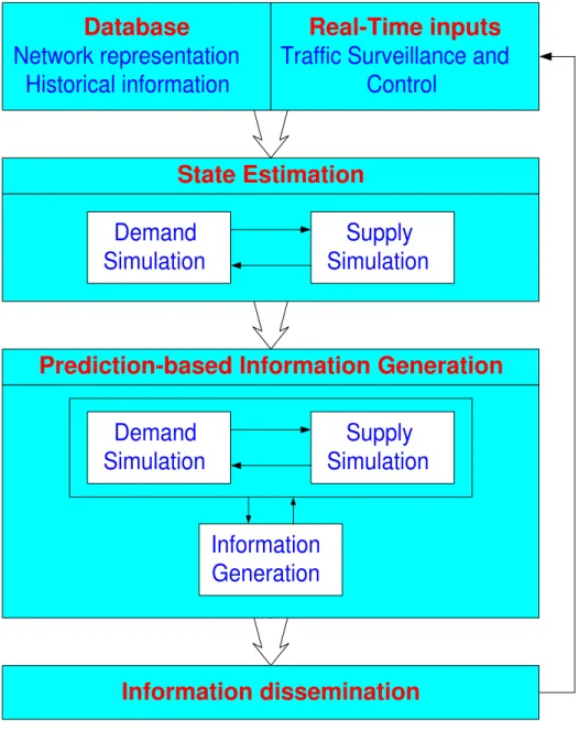
4.2 Overall Framework . . . 67
4.2.1 State Estimation . . . 71
4.2.2 Demand Simulation . . . 71
4.2.3 Supply Simulation . . . 74
4.2.4 Demand-Supply Interactions . . . 74
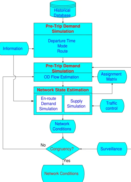
4.2.5 Prediction and Guidance Generation . . . 74
4.3 DynaMIT for Planning . . . 77
4.4 Calibration Variables . . . 83
4.4.1 Demand Simulator Parameters . . . 83
4.4.2 Supply Simulator Parameters . . . 86
4.5 Conclusion . . . 87
5 Case Studies 89 5.1 The Irvine Dataset . . . 89
5.1.1 Network Description . . . 90
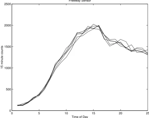
5.1.2 Data Description and Analysis . . . 91
5.1.3 DynaMIT Input Files . . . 94
5.2 Supply Side Calibration . . . 96
5.3 Demand Side Calibration . . . 96
5.3.1 Path Choice Set Generation . . . 97
5.3.3 Generating Seed O-D Flows . . . 98
5.3.4 Simplifying Assumptions . . . 100
5.3.5 Error Statistics . . . 100
5.3.6 Calibration Approach . . . 101
5.4 Validation of Calibration Results . . . 116
5.4.1 Validation of Estimation Capability . . . 116
5.4.2 Validation of Prediction Capability . . . 117
5.5 Summary and Conclusion . . . 119
6 Conclusion 121 6.1 Research Contribution . . . 121
6.2 Directions for Further Research . . . 122
6.2.1 Updating Model Parameter Estimates . . . 122
6.2.2 Simultaneous estimation . . . 123
6.2.3 Effect of number of sensors . . . 123
6.2.4 Handling incidents . . . 124
6.2.5 Driver behavior models . . . 124
6.3 Conclusion . . . 124
List of Figures
1-1 Dynamic Traffic Assignment . . . 17
1-2 The Calibration Problem . . . 18
2-1 General Calibration Framework . . . 28
2-2 The Fixed Point Problem . . . 31
2-3 Iterative Calibration Framework . . . 31
2-4 Overview of Inputs and Outputs . . . 37
2-5 O-D Flow Deviations . . . 40
3-1 Sequential O-D and Covariance Estimation . . . 58
3-2 Parameter Update Methodology . . . 61
4-1 The Rolling Horizon . . . 69
4-2 The DynaMIT Framework . . . 70
4-3 State Estimation in DynaMIT . . . 72
4-4 Prediction and Guidance Generation in DynaMIT . . . 76
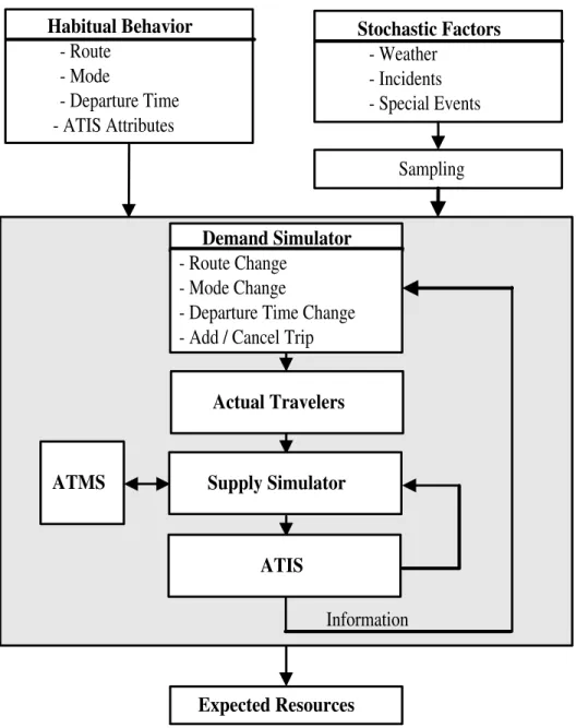
4-5 Framework for Travel Behavior . . . 78
4-6 Short-Term Dynamics . . . 81
4-7 Within-Day Dynamics . . . 82
5-1 The Irvine Network . . . 90
5-2 Primary O-D Pairs . . . 92
5-3 Primary O-D pairs . . . 92
5-4 Counts Variation Across Days: Freeway Sensor . . . 93
5-6 Subnetwork Calibration: Freeway Sensor . . . 97
5-7 Subnetwork Calibration: Ramp Sensor . . . 98
5-8 Subnetwork: Speed Comparison . . . 99
5-9 Route Choice Parameter Estimation . . . 103
5-10 Days 1, 2 and 4: Counts from 4:15 AM to 4:45 AM . . . 106
5-11 Days 1, 2 and 4: Counts from 4:45 AM to 5:15 AM . . . 107
5-12 Day 1: Counts from 5:15 AM to 5:45 AM . . . 108
5-13 Day 2: Counts from 5:45 AM to 6:15 AM . . . 109
5-14 Day 2: Counts from 6:15 AM to 6:45 AM . . . 110
5-15 Estimated Counts for 6:45 to 7:00 AM . . . 111
5-16 Estimated Counts for 7:00 to 7:15 AM . . . 111
5-17 Estimated Counts for 7:15 to 7:30 AM . . . 112
5-18 Estimated Counts for 7:30 to 7:45 AM . . . 112
5-19 Estimated Counts for 7:45 to 8:00 AM . . . 113
5-20 Estimated Counts for 8:00 to 8:15 AM . . . 113
5-21 Comparison of Time-Varying Freeway, Arterial and Ramp Sensor Counts114 5-22 Comparison of O-D Flows . . . 115
5-23 Predicted Counts for 7:30 AM to 8:00 AM . . . 118
List of Tables
5.1 Error in Fit to Counts for Varying Route Choice Parameters . . . 102
5.2 RMSN Errors from Four Estimations . . . 104
5.3 WRMSN Errors from Four Estimations . . . 104
5.4 Validation of Estimation Results . . . 116
5.5 Validation of Prediction Results . . . 117
A.1 Error Statistics for Day 1 Data (initialization) . . . 127
A.2 Error Statistics for Day 1 Data . . . 127
A.3 Error Statistics for Day 2 Data . . . 128
A.4 Error Statistics for Day 3 Data . . . 128
Chapter 1
Introduction
Physical and economic constraints are causing urban and suburban congestion re-lief solutions to move away from building more roads. Increasing attention is being focused on Advanced Traffic Management Systems (ATMS) and Intelligent Trans-portation Systems (ITS). Emerging Dynamic Traffic Management Systems (DTMS) attempt to optimize the utilization of existing system capacity by performing two basic functions. Firstly, such systems provide pre-trip and en-route information to drivers about anticipated network conditions for the duration of the proposed trip. In addition, the systems assist traffic control systems to adapt and adjust in real-time to dynamic traffic conditions.
A desirable feature of such systems is the ability to predict future traffic. Lack of knowledge about projected traffic conditions could render guidance or control initia-tives irrelevant or outdated by the time they take effect. Dynamic Traffic Assignment (DTA) is a critical component of such traffic prediction systems.
A DTA system models complex interactions between supply and demand in a transportation network. While the supply component captures traffic dynamics through the movement of packets on the road network according to aggregate traffic relation-ships, the demand component estimates and predicts point-to-point network demand and models driver behavior with respect to choice of departure time, mode and route. The demand simulator also models drivers’ response to information. The DTA sys-tem is designed to reside within a Traffic Management Center (TMC), and aid the
operator in locating congestion before it happens. This information will be valu-able in initiating preventive measures through a wide range of control strategies that include modifications to signal operations, diversion of traffic, and dissemination of route guidance information.
1.1
Motivation for Demand Calibration
Real-time applications of a Dynamic Traffic Assignment system typically utilize inputs from a traffic surveillance system to estimate and predict O-D flows (Figure 1-1). These predicted flows are then used as a basis to generate route guidance that may be disseminated to equipped drivers as traveler information. It is important to note that driver reaction to this guidance could merely cause spatial and temporal shifts in the predicted congestion, thereby invalidating the very prediction that influenced the guidance. The credibility of such systems therefore relies heavily on their ability to accurately estimate and predict traffic conditions under congested regimes, and to generate consistent route guidance. Consistency indicates that the predicted network state (in terms of congestion and travel times) matches that actually experienced by the drivers on the network.
Driver behavior and the underlying trip patterns are typically characteristic of the demographical and geographic section under study. Decisions regarding choice of route or departure time can depend on a host of observable variables (such as socio-economic characteristics, route attributes and value of time) and latent variables (like network knowledge and “aggressiveness”) that capture local conditions. The origin-destination flow patterns might be a function of the spatial distribution of residential and commercial zones. Accurate estimation and prediction of O-D flows and driver behavior therefore play key roles in the evaluation of driver response to guidance in the context of real-time traffic management. In order to ensure that the system reacts and behaves in a realistic manner when deployed at site, it is critical to calibrate these models against field data collected from the site of actual deployment. The calibration of the O-D estimation/prediction and route choice models is therefore critical to
Surveillance System Guidance and Control Generation Traffic Prediction O-D Estimation and Prediction Traffic Conditions Historical Data DTA System
establishing the credibility of the guidance system. Further, the close linkage between the route choice model and the O-D estimation and prediction model necessitates a joint calibration approach that will yield a consistent set of parameters across both models. This thesis focuses on the joint calibration of the demand simulator, comprised of the driver route choice and O-D estimation and prediction models.
1.2
Problem Definition and Thesis Objective
Figure 1-2 summarizes the input and output requirements of the calibration process. For the present, the calibration process can be visualized as a black box that uses available O-D flow estimates and several days of surveillance data as inputs. The outputs from the black box are the parameters in the route choice and O-D estimation and prediction models.
Offline Calibration a priori O-D Flows (From Surveys/Models) 'N' days of sensor data
Route Choice Parameters Time-Varying Historical O-D Flows
Error Covariance Matrices Autoregressive Factors
Figure 1-2: The Calibration Problem
Initial O-D flow estimates may be obtained through surveys, planning studies, or demand forecasting models. The quality of these estimates can vary significantly based on the methods used to generate them. Often, a good set of initial flow es-timates is not available, and has to be extracted from the surveillance data. The real-time data collected by the surveillance system can include time-dependent traf-fic counts, occupancies (a proxy for densities), speeds and queue lengths on links equipped with sensors. While the counts are typically used by the O-D estimation
and prediction model, the speeds, occupancies and queue lengths will be used to en-sure the accuracy of the supply-side model parameters that govern the movement of vehicles on the network.
The parameters in the route choice model are theoretically estimated from de-tailed disaggregate data obtained through travel surveys. Ideally, such surveys yield data pertaining to a host of attributes and socio-economic characteristics that might help explain individual route choice decisions. However, such a rich data set is seldom available. In most cases, we need to identify alternative methods of calibrating the route choice model parameters from available aggregate data. This data is often a manifestation of individual discrete choice decisions. The calibration approach should be able to accurately reproduce the observed aggregate data by adjusting the parame-ters in the individual driver behavior models. In this thesis, we propose a calibration methodology to jointly calibrate the parameters in the O-D estimation/prediction and route choice models using aggregate sensor data.
Each additional day of data contains valuable information about O-D flow patterns and driver behavior. The calibration framework takes advantage of the availability of several days of sensor data to generate the best parameter estimates. Various alternative approaches to using the available data are discussed. Demand patterns might also vary by day of the week, weather conditions, special events and incidents. Given data collected over an extended period of time, we would like to generate stratified O-D flow databases that cover such a wide range of demand conditions. Finally, recalling the real-time nature of the DTA system, we require a convenient means of updating the historical database as each additional day of observations are recorded.
1.3
Literature Review
Literature on the calibration of DTA systems is limited, and often relates to simple networks under uncongested traffic flow regimes. He, Miaou, Ran and Lan (1999) attempt to list the major sources of error in a DTA system, and lay out
frame-works for the offline and online calibration of the system. The proposed frameframe-works treat the calibration of the dynamic travel time, route choice, flow propagation and O-D estimation models sequentially. The authors consider a modified Greenshields model to explain dynamic travel time variations on freeway links, and split the travel times on arterials into a cruise time component and a delay component1. The
sug-gested calibration approach aims to minimize the “distance” between the analytically computed travel times and those measured by detectors. Further, the maximum like-lihood estimation procedure suggested for the calibration of the route choice model relies heavily on the availability of adequate survey or detector data about travelers’ route choices. This assumption would fail in several real cases, where only aggre-gate network performance measures (such as link counts) are available. A procedure similar to that adopted for the dynamic travel time models is applied for the flow propagation model, where link inflows and outflows are matched against detector data. While such a detailed level of model calibration might be preferred, the lack of such a rich disaggregate detector data set would often render the approach infeasible. In addition, the paper does not include the O-D estimation module, which constitutes a critical part of the demand simulator within a DTA system.
In a subsequent paper, He and Ran (2000) suggest a calibration and validation approach that focuses on the route choice and flow propagation components of a DTA system. This paper again assumes prior knowledge of time-dependent O-D matrices, and further simplifies the demand process by imposing the temporal independence of O-D flows between all O-D pairs. Also, the assumption of discrete data availability to allow a Maximum Likelihood Estimation of the route choice model is still a restriction on the practical applicability of the proposed approach. The two approaches reviewed thus far fail to address the overall problem of jointly calibrating the O-D estimation and route choice models.
An approach by Hawas (2000) uses an ad hoc ranking of DTA system components to determine the order in which these components must be calibrated. However, a linear relationship between components is inherently assumed, and cyclic data
change through feedback between components (as in the demand-supply interaction within a DTA system) is ignored. Further, the paper uses the components of a traffic simulator, and not a DTA system, as a case study.
The problem of O-D estimation itself has been the focus of several theoretical studies. Cascetta (1984) and Cascetta, Inaudi and Marquis (1993) extend a GLS-based static O-D estimation approach to the dynamic context2. The tests, however,
were performed on a linear network with no route choice. Also, no guidelines were provided for estimating the error covariance matrices that are critical estimation inputs.
Subsequent work by Ashok (1996), Ashok and Ben-Akiva (1993) and Ashok and Ben-Akiva (2000a) outlines a real-time O-D estimation and prediction framework based on a Kalman Filtering algorithm working with deviations of O-D flows from their historical values3. The approach is flexible so as to allow the explicit handling
of measurement errors and stochasticity in the assignment matrices. However, the theoretical development is tested on small scale networks with minimal or no route choice. Moreover, the initialization of the Kalman Filter requires historical flows, error covariances and autoregressive matrices, that are unknown at the beginning of the calibration process. While some approaches to estimating these quantities are suggested, they have neither been tested on real-sized networks, nor studied in detail. Van der Zijpp and Lindveld (2001) present a framework for O-D estimation that attempts to capture the phenomenon of peak-spreading in congested traffic networks by integrating both route and departure time choice into the estimation process. The core of this approach involves the estimation of a dynamic O-D matrix, whose cells are also associated with preferred departure times. A switch from the preferred de-parture time is associated with a certain disutility which is dictated by a schedule delay function. The estimation problem is modeled as a Space-Time Extended Net-2A detailed review of dynamic O-D estimation using Generalized Least Squares (GLS) is presented
in Section 2.4.
3Deviations attempt to capture the wealth of information about spatial and temporal
relation-ships between O-D flows contained in the historical estimates. The historical database would be synthesized from several days of data
work (STEN) built by replicating the physical network as many times as there are departure time periods. The replicated virtual origin nodes are duplicated further to represent the preferred departure interval, with links between the two sets of extra nodes depicting the realized departure intervals. The authors outline an iterative so-lution scheme based on the Frank-Wolfe user optimal assignment algorithm to identify a STEN that is consistent with the observed link flows. In a separate discussion, the authors mention some of the limitations and drawbacks of the methodology. Firstly, travel delays on links are approximated by a function of link inflows alone:
ta(qa) = t0a à 1 + a µ qa qcap ¶β! (1.1)
where tais the delay on link a, t0ais the delay under free-flow conditions, qais the inflow
for link a and qcap is the capacity of the link. While this function does not explicitly
capture congestion effects due to queuing, the authors suggest that a bottleneck model might be approximated by employing a large value for the constant β. However, the Frank-Wolfe algorithm was found to be incapable of handling the sensitive link delay functions resulting from large values of β. Other experimental observations point to the possibility of the iterative algorithm either cycling indefinitely between equivalent STENs, or terminating at a local minimum or saddle point. In addition, the numerical tests were performed on a small artificial network with assumed “true” O-D flow, preferred departure time and scheduled delay data. The route choice model was also assumed to be known.
Hazelton (2000) presents a Bayesian approach to the static O-D estimation prob-lem. Assuming Poisson-distributed O-D flows, the paper outlines a Maximum Likeli-hood Estimation procedure to estimate the unknown O-D flows from several days of link observations. The full likelihood expression is also simplified to yield a tractable estimation method that incorporates measurement errors in the observed link counts. The paper, however, suffers from several limitations. Firstly, the focus remains on static O-D estimation, and is therefore not directly suited to DTA scenarios.
Sec-ondly, the theoretical underpinnings are based on uncongested network conditions, which would be unrealistic in most real-time DTA applications. Lastly, the numerical tests described in the paper were performed on a small and simple grid network with 6 nodes and 14 directed links, along with synthetic data based on a known matrix of true O-D flows.
In a recent paper, Cascetta and Postorino (2001) evaluate different iterative solu-tion algorithms for the fixed-point O-D estimasolu-tion problem on congested networks. However, the paper does not focus on model calibration, and its scope is limited to static O-D estimation. As the paper provides key insights into the solution of fixed-point problems, we now review the concepts presented therein. Cascetta et al state the fixed-point formulation of the O-D estimation problem as:
f∗ = f (t∗) (1.2)
t∗ = argmin[F1(x, ¯t) + F2(H∗(c(f∗))x, ¯f )] (1.3)
The function f (.) in Equation 1.2 maps estimated O-D flows t∗ to estimated link
flows f∗. Equation 1.3 is the solution step that generates t∗ by optimizing over
the variable x, with F1(.) and F2(.) forming two terms in the objective function.
While F1(.) measures the distance between the O-D flow x and the target flow ¯t, the
function F2(.) measures the distance between the actual vehicle counts ¯f measured
at sensors, and the link flows resulting from the assignment of the demand vector x. In addition, the function H∗(.) assigns the O-D vector x first to paths flows (using
link cost function c(.)) and then to link flows.
The paper briefly looks at existence and uniqueness conditions for the composed fixed point problem outlined above. While these conditions are in general difficult to analyze mathematically, the authors state sufficient conditions that require both F1(.) and F2(.) to be continuous and convex, while at least one of them is strictly
Functional Iteration provides a simple iterative framework where the latest O-D flow estimates are fed back into the assignment model for the next iteration. The Method of Successive Averages, or MSA, is an alternative scheme that assigns weights to the results from each iteration:
tk= 1
kx
k+k− 1
k t
k−1 (1.4)
where the “filtered” flows tk are obtained by weighting the latest estimates xk, and
the filtered flows from the previous iteration tk−1. The iteration counter k is used to
generate the weights. While this method has the advantage of utilizing the estimates from all iterations, a potential drawback is that newer estimates are allotted lower weights. Consequently, “bad” initial estimates might be weighted higher, thereby low-ering the speed of convergence. The Method of Successive Averages with Decreased Reinitializations, or MSADR, is a modification of the MSA algorithm that reinitial-izes the algorithm’s “memory” with a frequency that decreases with the number of iterations. This acceleration step causes the algorithm to skip intermediate values and focus more on the later iterations that are closer to the solution. While the MSADR and MSA algorithms produce the same sequence of solutions in the limit, the convergence of the MSA (and hence of the MSADR) is difficult to establish. These algorithms are therefore suggested as heuristic approaches to solve the fixed point problem of interest. The authors mention the Baillon Algorithm as a fourth approach, but restrict themselves to the first three schemes for numerical testing.
The paper concludes that all three algorithms tested converged to the same fixed point even under stringent stopping tests. Functional iteration and MSADR out-performed MSA on speed of convergence. While these findings are indicative of the suitability of iterative schemes in solving fixed-point problems, they suffer from sev-eral limitations:
• The tests were based on a small and simple grid network.
• The study used synthetic surveillance data. O-D flow and sensor count mea-surements were generated artificially from known values.
• The Logit route choice model used a fixed travel time coefficient.
• The model estimated static O-D flows. While these might suffice for certain limited planning applications, they would be inadequate in a real-time DTMS scenario.
Conclusion
While there has been a profusion of theoretical works on DTA systems, the literature indicates that little work has been done on the calibration of their model components. Much of the results have been based on small and simple uncongested networks with little or no route choice, using synthetic data generated by adding a random term to some assumed “true” values. A few studies involving congested networks have either focused only on static O-D estimation, or have used simple networks consisting entirely of freeways. Above all, there seem to have been no previous attempts at jointly calibrating the parameters of the route choice model and the O-D estimation and prediction model. This thesis presents a framework for the joint calibration of the route choice and O-D estimation and prediction models within a DTA system. The proposed methodology is then applied to a case study from a large-sized network comprising of both freeways and arterials. The estimation and prediction abilities of the calibrated system are validated against real sensor data obtained from the field.
1.4
Thesis Outline
This thesis is organized as follows. In Chapter 2, we undertake a detailed explanation of the input and output requirements of the demand calibration process for a DTA system, and present the proposed calibration methodology. Chapter 3 explores issues pertaining to setting up a historical database of O-D flows and other inputs to the demand simulator. In chapter 4, we introduce DynaMIT, a state-of-the-art DTA-based prediction and guidance system, and DynaMIT-P, an application of DTA for planning. This chapter briefly describes the features, models and applications of the
DynaMIT and DynaMIT-P systems that form a basis for our case studies. Chapter 5 describes case studies that demonstrate the feasibility and robustness of the proposed calibration methodology when applied to large-scale networks, and presents valida-tion results that evaluate the estimavalida-tion and predicvalida-tion capabilities of the calibrated DynaMIT system. We conclude by stating some of the contributions of this research in Chapter 6, and outline directions for future research.
Chapter 2
Calibration Methodology
The dynamic traffic assignment system should possess the ability to accurately repli-cate traffic conditions as observed by the surveillance system. The primary objective of calibration is therefore to identify DTA model parameters and inputs that match the offline surveillance data available. In this chapter, we cast the calibration problem in an optimization framework, and discuss some important properties characterizing the problem and its solution. We later present an iterative approach to the joint calibration of the demand models within a DTA system.
Figure 2-1 summarizes the overall framework for the calibration of a DTA sys-tem. We first identify a set of parameters that requires calibration, and assign initial values to the same. The next step involves running the DTA system with the chosen parameters to generate simulated measures of system performance. This output is compared against the observed data obtained from the surveillance system, to eval-uate an objective function. Our parameter estimates are now modified, and a new optimization problem is solved. This process is continued iteratively until a predefined set of convergence criteria is satisfied.
The calibration framework can be viewed as a large optimization problem, with the final objective of matching various simulated and observed quantities:
M inimize
β, γ, xp
° °
° simulated quantity− observed quantity ° ° °
Initial Values DTA System Model Outputs Objective Function Optimization Observed Data Convergence Updated Parameter Values Analysis Yes No
The minimization can be over a combination of several network performance measures such as flows, speeds or densities. The simulated quantities are obtained through the following steps: xh = argmin[F1(xh, xah) + F2( h X p=h−p0 aphxp, yh)] (2.1) ap h = g(xp, β, γ, tt eq l ) (2.2) tteql = h(β, γ, xp) (2.3)
where β represents the route choice parameters, and γ the parameters in the supply simulator. Equation (2.1) forms the basic O-D estimation step in the calibration framework, and is itself an optimization problem with a two-part objective function. The function F1 measures the distance of the estimated flows xh from their target values xa
h, while F2 measures the distance of the measured counts yh from their
simulated values. The assignment matrices aph required by the O-D estimation module are outputs of the dynamic network loading model, and are functions of the as yet unknown O-D flows, the equilibrium travel times on each link (tteql ), the route choice parameters β and supply-side parameters γ (Equation (2.2)). Finally, the equilibrium travel times are themselves a function of the O-D flows, route choice parameters and supply-side parameters (Equation (2.3)). Equations (2.1) to (2.3) therefore capture the fixed-point nature of the calibration problem.
We now take a deeper look at the demand calibration process. Let us begin with the O-D estimation module, which forms an important part of the demand simulator within any DTA system. This module attempts to estimate point-to-point flows in the network based on link-specific traffic counts measured by the surveillance system. A key input for O-D estimation is the assignment matrix, the dimensions of which depend on the number of independent link sensors in the network and the number of O-D pairs to be estimated. Each element in the assignment matrix, therefore, represents the fraction of an O-D flow associated with a particular link, and is derived by simulating path flows in a dynamic network loading module. Path flows in turn
are obtained through a route choice model combined with knowledge of the O-D flows themselves, which we set out to estimate (Figure 2-2). The solution to the calibration problem is therefore a fixed point between the route choice fractions, the assignment fractions and the O-D flows, and necessitates an iterative solution approach.
2.1
Iterative Approach to Demand Calibration
The proposed iterative approach is illustrated in Figure 2-3. We use the route choice model as the starting point in our iterative framework. Ideally, the parameters in the route choice model should be estimated separately using a rich travel survey data set. Such a survey would typically contain information regarding individual drivers’ socio-economic characteristics and preferences, and attributes associated with the alternatives1. In the absence of such disaggregate data, we need a method of
estimating these parameters from aggregate data such as vehicle counts at sensors. The first step is to assume a set of initial values for the parameters in the route choice model. In order to generate an assignment matrix, we need additional information about path travel times and the O-D flows themselves. For a large network, the effort required to collect and store time-dependent path travel times throughout the period of interest can be prohibitive. We therefore simulate the assignment fractions using an initial seed O-D matrix. The route choice model uses the latest available travel time estimates to compute path choice probabilities2. Driver route choices are then
simulated to generate time-dependent assignment matrices. The assignment matrix and corresponding O-D flows are passed on to the O-D estimation module, the output of which is a new set of O-D flows.
This process raises two issues relating to convergence. The first issue deals with the assignment matrix. The newly estimated D flows (generated by the O-D estimation module) can be re-assigned to the network, using the original route 1The alternatives in this case being the different possible combinations of routes and departure
times.
2In the absence of initial travel time estimates, we might start the process with free-flow travel
Route Choice Model EstimationO-D Model
Dynamic Network Loading (DNL) Model
O-D Flows
Path Flows Travel Times
Assignment Fractions
Figure 2-2: The Fixed Point Problem
STOP START O-D Estimation Module Dynamic Network Loading (DNL) Model Route Choice Model Assignment Matrix Convergence Route Choice Parameters Convergence No No Yes Yes O-D flows Path travel times
Counts
choice model. The resulting assignment matrix is very likely to be different from the matrix used as input to the O-D estimation module. It is therefore essential to ensure consistency by iterating locally on the assignment matrix. A smoothing algorithm such as a weighted average3 (of the latest matrix estimate with estimates
from previous iterations) can be used as input for the subsequent iteration. A suitable termination rule should be determined in order to provide a stopping criterion. The second issue relates to the route choice parameters. The estimated O-D flows obtained thus far were based on the initial values assumed for the parameters in the route choice model. In the absence of disaggregate data, we are forced to employ aggregate approaches to estimate these parameters. Observing that link flows are indirect manifestations of driver route choice decisions, we iterate on the route choice model parameters until we are able to replicate fairly well the link flows observed at the sensors.
2.1.1
Iterative schemes
Cascetta and Postorino (2001) present three different algorithms4 to iteratively solve
the fixed point problem associated with static O-D estimation in congested networks. Their tests indicate that functional iterations and MSADR perform better than the MSA in terms of speed of convergence. No significant difference was noticed in the final solutions obtained. It is hard, however, to extend the findings to a larger dynamic problem. The suitability of the various algorithms will have to be evaluated through numerical testing.
The general structure of the iterative solutions consists of three basic steps: • Re-assign the current estimated O-D flows to obtain a new assignment matrix. • Compute a new assignment matrix using a smoothing algorithm.
• Use the smoothed assignment matrix to estimate new O-D flows.
3Typically, newer estimates are assigned higher weights than estimates from previous iterations 4Functional Iteration, Method of Successive Averages (MSA) and MSA with decreasing
The steps are repeated until a suitable set of termination rules is satisfied. The following sections provide a brief overview of the three iterative schemes.
Functional iteration represents the simplest form of the generic iterative algo-rithm outlined previously, with the latest assignment matrix estimate being used for the next iteration. Convergence is measured by the difference between successive O-D flow estimates across all O-D pairs. A simple modification in the above procedure can allow for the averaging of successive O-D flow estimates while computing the current estimate. Yet another algorithm can be visualized by averaging successive assignment matrices. However, this approach would involve the explicit evaluation and storage of several assignment matrices, and can be a burden on computational efficiency and storage.
The Method of Successive Averages (MSA) provides a way of assigning weights to successive O-D flow estimates, thereby speeding up the convergence of the iterative solution: xk∗ = 1 kx k+k− 1 k x k−1 (2.4) where xk∗
is the new flow vector after iteration k, xk is the estimate generated in
iteration k and xk−1 is the estimate from the previous iteration. Such a weighted
approach is often known as smoothing, and has been found to significantly improve convergence properties. It should be noted that the weight assigned to a new esti-mated flow vector decreases as the iterations progress towards a solution, implying that initial solutions are weighed more heavily than those closer to the true solution. Consequently, the algorithm can slow down dramatically in the final iterations before convergence. This drawback of the classical MSA algorithm is remedied in part by its variant, the MSA with Decreasing Reinitializations (MSADR), which erases the memory of the algorithm at predefined intervals. The frequency with which the memory is reinitialized decreases as the algorithm gets closer to the true solution it seeks. The effect of such an approach would be to skip intermediate solution steps, thereby ensuring faster convergence.
2.2
The Route Choice Model
The choice of route and departure time are important aspects in the modeling of incidents, response to information and the evaluation of guidance strategies. The route choice model captures key aspects of driver behavior in the context of dynamic traffic assignment, and attempts to replicate driver choice decisions using a set of explanatory variables. These variables can include route attributes such as travel times and cost components, as well as driver characteristics such as income level.
Route choices can be modeled at two levels. Pre-trip route choices are made before the driver embarks on the trip. At this stage, the driver has access to traffic information and guidance from a variety of sources such as radio traffic bulletins, the Internet, or a dedicated traveler information provider. The important aspect to note here is that drivers have the ability to change their departure time depending on the current information. Hence apart from changing the chosen route, the driver can also decide to leave sooner or later, in a bid to beat the rush. Other alternatives that are feasible at this point are a change of mode (say to public transit options), or to cancel the trip itself. Once the driver has embarked on the trip, however, several of the alternatives discussed above become unavailable. For example, drivers can no longer change their departure times. We now model en-route driver decisions that capture the phenomenon of path switching in response to real-time information. Such information could be available, for example, through in-vehicle units (for equipped drivers) or through Variable Message Signs (VMS) installed at specific locations on the network.
The route choice model operates on each driver’s choice set. This set contains all feasible combinations of departure times and routes. The choice probabilities for all alternatives within the choice set are evaluated using a discrete choice model5. It
further simulates this choice through random draws, and determines the chosen path. The aggregation of all such chosen paths will result in path flows by O-D pair, which are used by the Dynamic Network Loading model discussed next.
2.3
The Dynamic Network Loading Model
The path flows output by the route choice model are used by the dynamic network loading (DNL) model to create time-dependent assignment matrices. This step in-volves the assigning of path flows to the network, and counting the vehicles as they cross traffic sensors. The departure times of the counted vehicles are also tracked, as the matrices ap
h depend on the current interval h as well as the departure interval p.
Various analytical approaches with different underlying assumptions have been suggested for the DNL problem. Cascetta and Cantarella (1991a) approximate the behavior of all vehicles on path k in time interval h to be part of the same packet. In a modified continuous packet approach, the vehicles in a packet are assumed to be continuously spread between the “head” and the “tail” of the packet. Cascetta and Cantarella (1991b) suggest a further variation that allows packets to “contract” or “expand”, to help account for differing average speeds. All these approaches yield very complex expressions for the assignment matrix fractions, and introduce a high degree of non-linearity in the objective functions. Simulation provides us with a more tractable alternative. The path and departure time records for each vehicle can be tracked in a microscopic traffic simulator and later processed to obtain time-dependent assignment matrices. A more aggregate mesoscopic traffic simulator can also be used to achieve the same result.
2.4
The O-D Estimation Module
The O-D matrix estimation problem involves the identification of a set of O-D flows that, when assigned to the transportation network, results in link flows that closely match observed flows. The input data can be obtained from various sources, derived from different processes and characterized by different error component structures. We therefore need a unified approach that extracts the maximum information out of the available data in a statistically efficient manner.
2.4.1
Inputs and Outputs
Figure 2-4 illustrates the basic inputs and outputs for an O-D estimation model. This model obtains initial O-D flow estimates from a historical database (the generation of this database is a part of our calibration exercise). In addition, the module gets a vector of link counts from the surveillance system6. In an offline application, such
as calibration, link counts for the entire analysis period would be available to the model. However, in a real-time context, at the end of each interval h, only the counts measured during that interval will be reported by the surveillance system. Finally, the model either gets, or computes, a set of assignment matrices7. By comparing
the link counts measured by the sensors with the counts obtained by assigning the estimated or a priori O-D flows to the network, the O-D estimation model updates these estimates. While the offline estimation can attempt to estimate flows for all T intervals simultaneously, the real-time estimation necessarily proceeds sequentially through the intervals.
2.4.2
Preliminary Definitions
We begin by introducing some basic definitions that will be followed henceforth in this thesis. Consider T , the analysis period of interest, to be divided into T subintervals 1 . . . T of equal length. The network is represented by a directed graph that includes a setN of consecutively numbered nodes and a set of numbered links L. The network is assumed to have nLK links, of which nl are equipped with sensors. There are nOD O-D pairs of interest.
We denote by xrh the number of vehicles between the rth O-D pair that departed from their origin in time interval h, and by xH
rh the corresponding best historical
estimate. A historical estimate typically is the result of estimation conducted during previous days. Further, let the corresponding (nOD ∗ 1) vector of all O-D flows and their corresponding historical estimates be denoted as xh and xHh respectively. Let 6More generally, the inputs are a set of direct and indirect measurements, as described shortly. 7As mentioned in Chapter 1, an assignment matrix maps origin-destination flows into link flows.
O-D MATRIX ESTIMATION Estimated O-D Flows Assignment Matrix Link Counts Historical O-D Flows
ˆ
xh represent the estimate of xh. Finally, denote by ylh the observed traffic counts at sensor l during time interval h, and by yh the corresponding (nl ∗ 1) vector.
Traffic measurements fall into two broad categories: • Indirect measurements
• Direct measurements
Indirect measurements contain information about the quantities we wish to estimate, but are not direct observations of the quantities themselves. Our objective is to estimate O-D flows. Observations of link counts at traffic sensors, for example, would contain information about the O-D flows that caused them. In fact, link counts constitute the most common type of indirect measurements. Link flows can be related to the O-D flows through a set of assignment matrices:
yh =
h
X
p=h−p0
aphxp + vh (2.5)
where yh are the link counts observed in time interval h, xp is a matrix of O-D flows
departing in interval p, ap
h is an assignment matrix that relates flows departing in
interval p to counts observed in interval h, and vh is a random error term. p0 is the
maximum number of intervals required by a vehicle to clear the network. Let the variance-covariance matrix of vh be denoted as Vh.
The indirect measurements represent nl equations in n
OD unknown variables.
Typically, nOD is much larger than nl. In order to be able to estimate the n
OD
unknown flows, we supplement the indirect measurements with direct measurement “observations”.
Direct measurements provide preliminary estimates of the unknown O-D flows. We therefore express a direct measurement as follows:
where xa
h is the starting estimate of matrix xh, and uh is a random error term. We
now have a total of (nl + nOD) equations to solve for the nOD unknown flows. Let the variance-covariance matrix of uh be denoted as Wh.
2.4.3
Deviations
It should be noted that Equation (2.6) only provides a means of including additional observations on the O-D flows. The a priori estimates xah can have a variety of functional forms (Ashok (1996)). Assume that we possess a historical database of O-D flows synthesized from several days of data. Such a database would contain valuable information about the spatial and temporal relationships between O-D flows. In order to accommodate this structural information into the new estimates, we work with deviations of current O-D flows from their historical values ( Figure 2-5 ):
xah = xHh + h−1 X p=h−q0 fhp(xp − x H p ) (2.7) where fp
h is a matrix that relates deviations in time interval p to the current time
interval h. Stated as deviations,
∂xa h = h−1 X p=h−q0 fp h∂xp (2.8)
The measurement equations get modified as:
yh− h X p=h−p0 ap hx H p = h X p=h−p0 ap h(xp − x H p ) + vh (2.9) yh− yH h = h X p=h−p0 ap h∂xp + vh (2.10)
time period
O-D
flows
h
h-1
where yH h = Ph p=h−p0a p hx H
p . We are now ready to synthesize O-D flow estimates by
combining the information contained in the direct and indirect measurements. The following sections review two approaches to O-D estimation from the literature. The first is a generalized least squares approach, while the second uses a Kalman Filtering technique.
2.4.4
Generalized Least Squares (GLS) Approach
The classical GLS estimator minimizes the “distance” between the estimated O-D flows and the a priori flows, while simultaneously ensuring that the measured link flows are as close as possible to the newly assigned link flows (the link flows ob-tained by assigning the newly estimated O-D flows to the network). The indirect measurements are first adjusted for link flow contributions from previous intervals:
yh− h−1 X p=h−p0 ap hˆxp = a h hxh + vh (2.11)
The direct measurement equations are maintained as is:
xa
h = xh+ uh (2.12)
The combined system of indirect and direct measurements can be expressed in matrix algebra as:
yh −Ph−1 p=h−p0a p hˆxp xah = aph In OD xh + vh uh or
Yh = Ahxh + ²h (2.13) The error covariances Vh and Wh associated with the indirect and direct measure-ments can be represented by a single covariance matrix:
Ωh = Vh 0 0 Wh
The above structure for Ωh assumes that the measurement errors associated with the indirect and direct measurements are not correlated. This would be a reasonable assumption in most cases, as the two types of measurements are obtained from two entirely different measurement processes. The flow estimates are then given by:
ˆ
xh = argmin[(Yh − Ahxh)0Ω−1h (Yh − Ahxh)] (2.14)
Ω−1h can be interpreted as a weighting matrix. The weights for each measurement (indirect or direct) reflect our confidence in the measurement process. For example, we might discount the information contained in the a priori O-D flows because they were derived from a static planning study. The corresponding high variance in the direct measurement errors would manifest themselves as a low weight. On the other hand, we also capture the effect of measurement errors in the counts recorded by traffic sensors. A good sensor would therefore be associated with a lower error variance, thereby implying a higher weight. The variability of the errors is thus captured through the covariance matrix Ωh.
The estimator we have just described is a sequential estimator, in that it treats the T time intervals one at a time. In other words, the estimates ˆxh−1, ˆxh−2, . . . obtained for past intervals h− 1, h − 2, . . . are kept constant when estimating flows for current
interval h. Expanding Ωh, we can state the optimization problem as: ˆ xh = argmin[(xh − xah)0W−h1(xh − xah) +(yh − h−1 X p=h−p0 ap hxˆp − a h hxh) 0V−1 h (yh− h−1 X p=h−p0 ap hxp − a h hxh)] (2.15)
While this approach has advantages from a computational standpoint, we might be able to obtain more consistent estimates by estimating the flows for all T time intervals simultaneously8. The equivalent of equation (2.14) would then be:
(ˆx1, ˆx2, . . . , ˆxT) = argmin[ T X h=1 (Yh − Ahxh)0Ω−1 h (Yh − Ahxh)] (2.16)
where the minimization is over xi ≥ 0 ∀i = 1, 2, . . . , T . Again, we can expand Equation (2.16) as: (ˆx1, ˆx2, . . . , ˆxT) = argmin T X h=1 [(xh − xah)0W−1h (xh− xah)] + T X h=1 [(yh− h X p=h−p0 ap hxp) 0V−1 h (yh − h X p=h−p0 ap hxp)] (2.17)
It should be noted that Equations (2.16) and (2.17) represents a much bigger optimization problem when compared with Equations (2.14) and (2.15). In a practi-cal application, computational considerations might drive us towards the sequential estimator.
2.4.5
Kalman Filter Approach
The Kalman Filter approach (Ashok and Ben-Akiva (2000b)) provides a convenient O-D estimation and prediction method for real-time applications as well as offline estimation. This approach views the O-D estimation problem as a state-space model9
8Simultaneous estimation gains significance in offline applications such as model calibration. 9The reader is referred to Gelb (1974) for an exhaustive coverage of state-space models.
which consists of two equation systems: M easurementEquation :Yh = AhXh + vh (2.18) T ransitionEquation :Xh+1 = ΦhXh + Wh+1 (2.19) where Xh = h ∂x0 h ∂x 0 h−1 · · · ∂x 0 h−s i0
The transition equation is based on an autoregressive process similar to Equation (2.7). The state variables Xh used in the above formulation correspond to an
aug-mented state approach that combines the advantages of both simultaneous and se-quential estimators while reducing the heavy computational load associated with si-multaneous estimation. The term Ah is a suitably constructed matrix of assignment fractions.
Assume that the initial state of the system X0 has known mean ¯X0 and variance P0. The system of measurement and transition equations can then be combined into a sequence of steps that easily integrate a rolling horizon:
Σ0|0 = P0 (2.20) Σh|h−1 = Φh−1Σh−1|h−1Φ0 h−1+Qh−1 (2.21) Kh = Σh|h−1A0 h(AhΣh|h−1A 0 h + Rh) −1 (2.22) Σh|h = Σh|h−1 − KhAhΣh|h−1 (2.23) ˆ X0|0 = X¯0 (2.24) ˆ Xh|h−1 = Φh−1Xˆh−1|h−1 (2.25) ˆ Xh|h = Xˆh|h−1 + Kh(Yh − AhXˆh|h−1) (2.26) The term ˆXh|h−1 represents a one-step prediction of the state Xh, and signifies the
best knowledge of the deviations Xh prior to obtaining the link counts for interval h. This prediction is achieved through the autoregressive process described by Equation
(2.25). Σ
h|h−1 denotes the variance of ˆXh|h−1, and depends on the uncertainty in both
ˆ
Xh−1|h−1 as well as the error in the autoregressive process (Equation (2.21)). The role of the Kalman gain matrix Kh is explained intuitively by Equation (2.26). Kh helps update the one-step prediction ˆXh|h−1 with the information contained in the new measurements Yh.
2.4.6
GLS vs the Kalman Filter
The Kalman Filter yields a convenient and elegant sequential methodology to update the O-D flow estimates and error covariance matrices with data from successive time intervals. The advantages of simultaneous estimation can also be easily integrated into the estimation framework through the technique of state augmentation, and is well suited to function in a rolling horizon10. In addition, the transition equation
inherently embeds a prediction step based on a rich autoregressive process. The Kalman Filter approach is therefore a joint O-D estimation and prediction model, and is an obvious choice within a real-time DTA-based traffic prediction and guidance system.
While the advantages are many, the Kalman Filter might suffer from some limita-tions in a calibration framework. The inputs to the Kalman Filter algorithm include a historical database of O-D flows, covariances of the initial flows, error covariance matrices and autoregressive matrices. As several of these input parameters are likely to be unavailable in the initial stages of a calibration application, we need alternative ways of initializing the Kalman Filter before it can be deployed on site. Further, Equations (2.20) to (2.26) represent repeated matrix operations involving matrices of very large dimensions, and could potentially render an iterative calibration scheme computationally expensive and infeasible.
A practical solution to the above problem might be suggested by Ashok (1996), which presents a derivation of the Kalman Filter algorithm from a GLS approach and establishes the equivalence of the two methods for discrete stochastic linear processes.
Chapter 3 explores this approach in detail, and addresses issues related to initializing the calibration process, and the availability of data.
2.5
Supply-Side Calibration
While the focus of this thesis remains the calibration of the model parameters on the demand side of a dynamic traffic assignment system, one should note that a DTA system models equilibrium in the traffic network by modeling the interactions between the demand and supply components. Indeed, the assignment matrix, which is a crucial input to the O-D estimation module, is an output of a supply simulation that captures traffic dynamics and simulates driver decisions in the context of capacity constraints. It is therefore necessary to place the problem of demand calibration within an even larger overall calibration framework.
The demand calibration framework presented here assumes the availability of a calibrated supply simulator. The DTA calibration process should capture the close interaction between the demand and supply components, and should attempt to es-timate the parameters in both classes of models jointly. While we do not present detailed discussions on the calibration of the supply model parameters in this work, some results on this topic may be found as part of the case studies in Chapter 5.
2.6
Model Validation
A good indication of a valid model is its ability to predict future system behavior. Model validation is therefore a critical final step in the calibration framework. The calibration process might yield consistent and efficient parameter estimates that fit the observed data. However, it is necessary to ensure that the calibrated system continues to perform in a satisfactory manner when faced with fresh information from the surveillance system. This issue is particularly important in the context of a Traffic Management Center, where the calibrated DTA system must possess the robustness to deliver accurate estimations and predictions in the face of real-time
fluctuations in the measurements. These fluctuations can consist of either day-to-day variations in traffic flows, or can represent significant deviations from normal conditions due to accidents, incidents, weather or special events.
It is often too expensive or difficult to conduct separate data collection efforts for calibration and validation. In such situations, we are forced to utilize the available data wisely to achieve both objectives. We might then divide the available data into two sets. While the first set would be used to estimate our model parameters, the second might be used as the basis for model validation. Such an approach might also help eliminate some of the effects specific to a particular data set.
It should be noted that discrepancies between model predictions and system out-put after implementation might indicate the necessity to re-calibrate the model with new data.
2.7
Conclusion
In this chapter, we formulated the overall DTA calibration process as an optimization problem, and presented an integrated framework for the joint calibration of the de-mand models within a DTA system. We discussed the roles played by the components within the demand and supply simulators, and analyzed the inputs and outputs at each calibration step. We concluded with a note on model validation and the larger calibration picture. The next chapter will explore some of the issues relating to start-ing the calibration process in the absence of reliable initial parameter estimates, and focus on the use of multiple days of surveillance data to generate efficient estimates. Subsequent chapters will present case studies that demonstrate the feasibility and robustness of the proposed calibration methodology.
Chapter 3
Creating a Historical Database
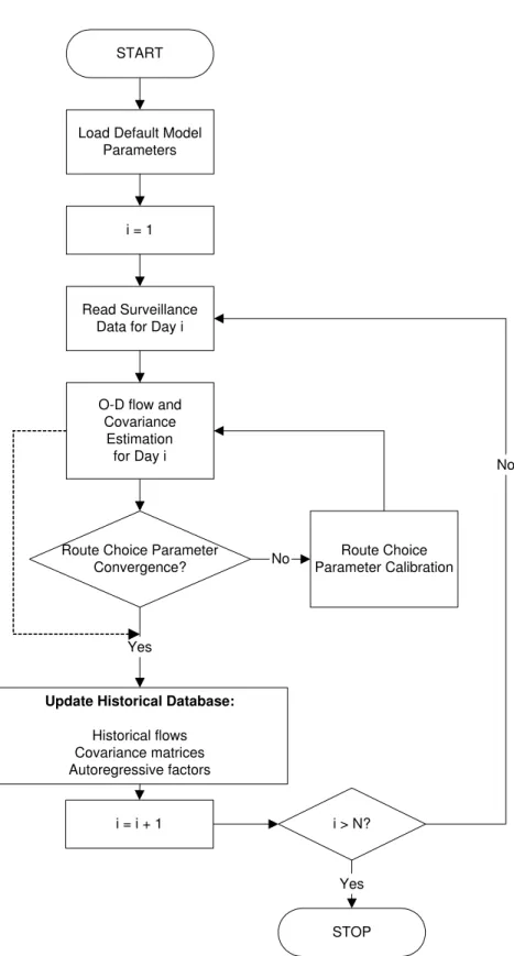
In Chapter 2, we presented an iterative approach to the calibration of the demand models within a DTA system. However, the component steps in this process had several input requirements that might not be readily available. In this chapter, we present approaches to starting the calibration process in such cases, and outline sim-plifications that would allow us to estimate the missing inputs from a single day of data. We further discuss ways of obtaining efficient parameter estimates from the en-tire set of available data spanning several days of surveillance records, and conclude with a section detailing the process of updating our historical database of O-D flows, error covariances and autoregressive factors with each additional day of estimations. We begin by briefly reviewing the input requirements of the O-D estimation mod-ule that forms the core of the demand calibration routine.
3.1
The O-D Estimation Module
The inputs to the O-D estimation module are the a priori O-D flows xa
h, the sensor
counts yh, the assignment matrices aph and the variance-covariance matrices (Vh and Wh) associated with the direct and indirect measurement errors. The outputs are the estimated O-D flows. The new O-D flows can be estimated based on Cascetta’s
GLS formulation (Cascetta (1984) and Cascetta et al. (1993)). (ˆx1, ˆx2, . . . , ˆxT) = argmin T X h=1 [(xh − xah)0W−1h (xh− xah)] + T X h=1 [(yh− h X p=h−p0 ap hxp) 0V−1 h (yh − h X p=h−p0 ap hxp)] (3.1) ˆ xh = argmin[(xh − xa h) 0W−1 h (xh − x a h) +(yh − h−1 X p=h−p0 ap hxˆp − a h hxh) 0V−1 h (yh− h−1 X p=h−p0 ap hxp − a h hxh)] (3.2)
Equation (3.1) solves for flows in several time intervals simultaneously. This in-volves the estimation of (nOD ∗ T ) unknown O-D flows, where nOD is the number of O-D pairs, and T is the number of time intervals in the period of interest. The large number of unknown quantities increases the computational burden tremendously. Equation (3.2) sequentially estimates flows in successive time intervals. Note that both approaches assume a knowledge of xa
h, Vh and Wh. The following sections
address the issue of generating these matrices.
3.2
Generating a priori O-D flow estimates (x
ah
)
The a priori O-D flows provide direct measurement observations of the true flows. Apart from supplementing the set of indirect measurements, these observations help capture temporal relationships and spatial travel patterns among the O-D flows. It is therefore imperative that we include these direct measurements, even if the number of indirect measurements is adequate to solve for the O-D flows. Equation (2.6) allows us to compute the a priori flows in a variety of ways. The most straightforward possibility is to use flows from a historical database as starting guesses. Since our aim, however, is to generate these historical flows, we need to look elsewhere for our direct measurements. In a strict sense, the direct measurements are not realobservations. We simply attempt to create realistic measures that might add to the information already available. While several formulations for xa
h can be visualized, we
look at a few possibilities. The most straightforward option for a direct measurement is to use available O-D flow estimates:
xa
h = x H
h (3.3)
In the absence of such time-dependent historical flow estimates, an alternative is to use the flows estimated for interval h− 1 as the starting point for interval h (Cascetta et al. (1993)):
xa
h = ˆxh−1 (3.4)
However, such a formulation does not account for any patterns in the underlying demand process. Let us for the present assume that we have good historical O-D flow estimates1. Ashok (1996) hypothesizes that the ratio of interval-over-interval O-D
flows is stable on a day-to-day basis, and suggests:
xah = (xHh /xH
h−1)ˆxh−1 (3.5)
We might further hypothesize that the O-D flows for interval h may be influenced by flows in several preceding intervals. This prompts us to consider a modification of (3.5) that spans several prior intervals:
xa h = h−1 X p=h−q0 τp(x H h /x H p )ˆxp , X p τp = 1 (3.6)
Another method of capturing temporal dependence between the O-D flows is to build an autoregressive process of degree q0 into the a priori estimates (Ashok (1996)):
xa h = h−1 X p=h−q0 fp hˆxp (3.7) The (nOD ∗ nOD) matrix fp
h in Equation (3.7) captures the effects of xp on xh, and
helps accommodate temporal effects in O-D flows. A big drawback of this method is that the wealth of information contained in the historical estimates is ignored. By moving to deviations, we can integrate this information into the current estimation problem: xa h = x H h + h−1 X p=h−q0 fp h(ˆxp − x H p ) (3.8)
The new target O-D flows xa
h now contain information about flows in past intervals.
The matrix fhp is now an (nOD ∗ nOD) matrix of effects of (xp − x H
p ) on (xh − x H h ).
This formulation captures correlation over time among deviations, which arise from unobserved factors (such as weather conditions or special events) that are themselves correlated over time.
An important question that needs to be answered pertains to starting the process. It should be noted that historical O-D estimates or autoregressive factors might not be available while processing the first few days of data. While Equation 3.8 is clearly one of the best ways to obtain the target O-D flows, we need to explore other ways of obtaining xah until we have sufficient data to estimate xHh and fhp.
Consider the first day of data. We clearly need some reasonable flow estimates for the first interval. Let us denote by xSh a set of seed matrices of O-D flows. These matrices represent the flow estimates available at the beginning of the calibration process, and can be dynamic or static. A dynamic set of seed matrices will allow us