HAL Id: inria-00616154
https://hal.inria.fr/inria-00616154
Submitted on 23 Jan 2014
HAL is a multi-disciplinary open access
archive for the deposit and dissemination of
sci-entific research documents, whether they are
pub-lished or not. The documents may come from
teaching and research institutions in France or
L’archive ouverte pluridisciplinaire HAL, est
destinée au dépôt et à la diffusion de documents
scientifiques de niveau recherche, publiés ou non,
émanant des établissements d’enseignement et de
recherche français ou étrangers, des laboratoires
Comparison of the endocast growth of chimpanzees and
bonobos via temporal regression and spatiotemporal
registration
Stanley Durrleman, Xavier Pennec, Alain Trouvé, Nicholas Ayache, José Braga
To cite this version:
Stanley Durrleman, Xavier Pennec, Alain Trouvé, Nicholas Ayache, José Braga. Comparison of the
endocast growth of chimpanzees and bonobos via temporal regression and spatiotemporal registration.
Miccai Workshop on Spatio-Temporal Image Analysis for Longitudinal and Time-Series Image Data,
2010, Beijing, China, China. �inria-00616154�
Comparison of the endocast growth of
chimpanzees and bonobos via temporal regression
and spatiotemporal registration
S. Durrleman1,2,3, X. Pennec2
, A. Trouvé3
, N. Ayache2
, and J. Braga4
1
Scientific Computing and Imaging (SCI) Institute, University of Utah, USA
2
INRIA - Asclepios Team-Project, Sophia Antipolis, France
3
Centre de Mathématiques et Leurs Applications (CMLA), ENS-Cachan, France
4
Lab. d’anthropobiologie, CNRS-Université Paul Sabatier, Toulouse, France
Abstract. In this paper, we aim at characterizing and quantifying the differences between the growth of bonobos (Pan paniscus) and chim-panzees (Pan troglodytes). We use a collection of endocasts of wild-shot animals of both species. Each sample has been associated with a dental age, as a common temporal marker. To compare the endocasts, we used the current-based metric which allows us to quantify the shape differences withoutthe need to find homologous landmarks on the surfaces. First, we perform a temporal shape regression, which estimates a typical growth scenario of the endocast for the bonobos and the chimpanzees. Then, a spatiotemporal registration scheme is used to quantify the differences between these two growth scenarios. The variations are decomposed into one morphological deformation and one time warp. The morphological deformation accounts for the anatomical differences independently of the age. The time warp accounts for the change of the dynamics of growth. It shows that the growth speed of the bonobos at juvenility is more than twice less than the one of the chimpanzees. This estimation gives more insights into the developmental delay observed in the bonobos growth.
1
Introduction
This paper aims at characterizing the differences of growth patterns between the two closest human relatives: the bonobo (Pan paniscus) and the chimpanzee (Pan troglodytes), two species of the genus Pan. According to phylogenetic stud-ies [17], these two specstud-ies share a common ancestor, which used to live at least two millions years ago. By comparison, the common ancestor of humans, chim-panzees and bonobos used to live at least ten millions years ago.
Bonobos were discovered to science in 1929. Since then, both morphological and behavioral studies tend to show that the bonobo is a “juvenilized” version of the chimpanzee [13]. Indeed, body growth is considered to be retarded in bono-bos compared to chimpanzees, a feature corresponding to their delay in motor development during the first years of postnatal life [8]. The adult bonobo skull shows a decreased facial prognathism and teeth with a reduced sexual dimor-phism [14]. Bonobos are also characterized by a longer dependency of the child
on the mother [16]. These studies lead to put forth the “bonobos hypothesis”, which assumes the bonobo to be a dwarfed version of the chimpanzee. To inves-tigate to which extent this hypothesis may be true, one must carefully analyze the difference between the growths of both species, called ontogenesis. Unfortu-nately, the lack of reliable data, in particular for the bonobos, has made difficult so far the study of the ontogenesis of both species and their comparison.
In this study, we focus on the endocasts of the specimens, which is a mould of the endocranium. The surface of this mould provides a replica of the inner surface of the skull, and therefore has often played an important role for the study of the evolution of the brain in fossil mammals [12,10]. We use here a cohort of about 60 endocasts of wild-shot animals of each species, which is among the largest collection available. It has been observed in [7] that the sequences of teeth emergence in bonobos and chimpanzees are essentially identical. This gives a way to estimate the “dental age” of each skull, as a common growth marker.
In this paper, we detect and compare geometrical growth patterns in these data using the methodology recently introduced in [3,2]. First, a shape regression method enables to estimate a typical growth scenario for each species. Second, a spatiotemporal registration scheme is used to compare the two growth scenarios both in terms of morphological changes and in terms of different growth speeds. This yields a quantitative estimation of the possible morphological delay of the bonobos with respect to the chimpanzees growth, which is the main feature we want to measure in regards to the bonobos hypothesis.
Last but not least, the implementation of this methodology uses the metric on currents to quantify shape dissimilarity [15,5,2] (although other metric could be also compatible with the proposed methodology). This allows us to compare endocasts without relying on the choice of landmarks points on the surface. This differs from usual methods used in physical anthropology [9,11], which uses the so-called geometric morphometric analysis as initiated in [1]. Here the shape comparison is expert-independent. The subsequent analysis is not biased by the choice of the landmarks and the inherent inter-expert variability. The geometry of the endocast is considered as a continuous surface and includes the direction of the normals. Moreover, the analysis of shape differences can be used afterwards to drive the search of significant anatomical landmarks like the ones which highlight the most striking differences between species.
The paper is organized as follows. In Section 2, we present the methodology used for the analysis of the endocasts data. In Section 3, we show that this method enables to estimate a typical growth scenario for the two species and to measure both their morphological differences and their different growth speeds.
2
Methodology
As explained in [2], the proposed methodology is subject-specific. This means that every subject, here every species, is supposed to evolve in the same atempo-ral morphological space (a given reference frame provided by its own coordinate system). The growth of each species is described by a time-varying function
χt(x) (for any time t and point in space x) in its own coordinate system (See
Fig. 2). The growth scenarios of two species may differ in two ways. First, dif-ferent species have difdif-ferent morphologic features, independently of the age of the individuals. Second, the dynamics of the growth scenarios may be different for different species: one anatomical development may occur at different speed, thus leading to developmental delay or advance. The first difference is described by a morphological function φ(x) (spatial deformation) which maps the refer-ence frame (i.e. morphological space) of one species into the one of the second species. The change of dynamics is described by a time-warp ψ(t) which is a 1D-diffeomorphism (smooth deformation which prevents time-reversal) which maps the age of one species t to the corresponding age of the second species ψ(t). This function changes the speed the growth of the species in a non-linear way. Eventually, the differences between two growth scenarios is described by the spatiotemporal deformation (φ, ψ) which best aligns the scenarios.
Two subjects have been scanned twice (one subject per rows, one
time-point per column).
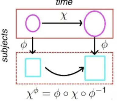
Fig. 1. In the subject-specific approach, one considers that one subject is “circle” and the other is “square”: the difference between both subjects is a single function φ, which maps circles to squares, in-dependently on time. The evolution of the first sub-ject is described by a function χ which maps a small circle to a big circle. The evolution of the second subject is then described by the function χφwhich
maps a small square to a big square. Once regis-tered into the “morphological space” of the squares, the circle evolution may still differ from the square one by a change of the speed of the evolution. This variations will be captured by the time-warp ψ.
2.1 Temporal shape regression
The growth scenario of one species is described by the growth function χt, a
3D-deformation of the underlying space. Given a baseline shape S0, this function
induces a continuous shape evolution S(t) = χt(S0) for t in the time interval of
interest. Given a discrete set of observed shapes (Si) associated to time-points ti
and a baseline S0, one aims at estimating the continuous growth function χtin
a least square sense (i.e. by minimizing the sum of squared differences between each shape Si and the growth scenario at time-point ti: S(ti) = χti(S0)):
J(χ) =X
ti
d(χti(S0), Si) 2
+ γχReg(χ) (2.1)
where d is a similarity measure between shapes, Reg(χ) a regularity term and γχ a trade-off between regularity and fidelity to data. Here we use the distance
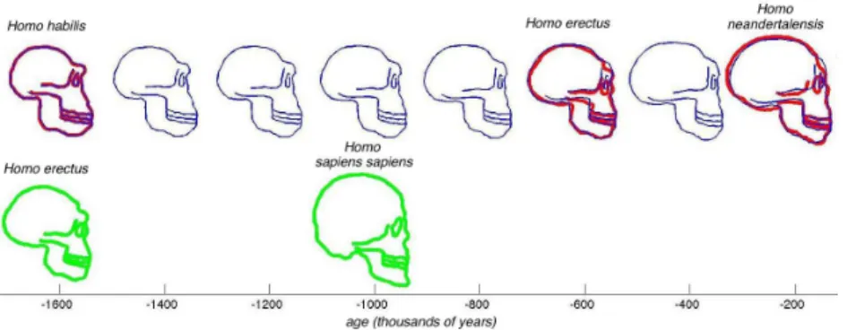
Fig. 2.Example of shape regression on profiles of hominid skulls (in red). We choose the australopithecus profile as the baseline S0. The temporal regression computes a
continuous shape evolution S(t) (in blue) such that the deformed shape matches the observations at the corresponding time-points. If several shapes are associated to the same time-point, they are averaged during the estimation of the regression.
shapes like curves or surfaces without the need for introducing landmarks on shapes. This metric depends on a scalar parameter λW, which is the typical
spa-tial scale under which geometrical variations are considered as noise (see [15,4,2] for more details). The regularity term is given as the total kinetic energy of the deformation [5,2]. In the framework of the RKHS [2], the regularity of the defor-mation is controlled by a scalar parameter λχ, which is the typical scale under
which points move in a correlated manner. This selects a group of deformations whose spatial frequencies fall within a given band. The more concentrated the “spectrum” of the deformation at the band limit, the higher the regularity term Reg(χ). Once the scale λχ is fixed, the trade-off γχ controls the goodness of fit
achieved by the deformation within the group which minimizes the criterion. For γχ → ∞, the resulting deformation will be identity map (no deformation)
independently of the scale λW. For γχ→0, data will be fit as closely as possible
without penalizing irregular deformations within the group. The baseline S0 is
usually chosen as the smallest shape associated to the earliest age.
As an illustrative example, we applied this temporal shape regression method on a set of 2D profiles of hominid skulls (segmented from images obtained at www.bordalierinstitute.com). Results are shown in Fig. 2.
2.2 Spatiotemporal registration
Once the temporal shape regression has been performed separately for each species, we end up with two growth scenarios: B(t) and C(t) (described by two growth functions χb
t and χct). The morphological deformation φ maps the
chim-panzee morphological space to the bonobos one: is deforms the shapes C(t) into φ(C(t)) for any age t. The time-warp ψ(t) change the dynamics of the chimpanzee growth by mapping the age t to the age ψ(t). The spatiotemporal deformation of the chimpanzee growth is given as: ˜C(t) = φ(C(ψ(t))). One aims at estimat-ing the spatiotemporal deformation (φ, ψ) which best aligns the chimpanzees growth to the bonobos one. For this purpose, we sample the evolution of B as a collection of B(τi) for linearly spaced time-points τi. A Maximum A Posteriori
J(φ, ψ) =X
τi
d(φ(C(ψ(τi))), B(τi)) 2
+ γφReg(φ) + γψReg(ψ) (2.2)
where d is the distance between shapes given by the metric on currents like for the regression function, Reg(φ) and Reg(ψ) the regularity terms of the morphological deformation and the time-warp, γφ and γψtwo scalar parameters which balance
the weight of the fidelity-to-data and the regularity terms. The regularity terms are the total kinetic energy of the diffeomorphism in the 3D domain for φ and 1D domain for ψ. In the same framework as the regression function, they depend on two scalar parameters: λφ which determines the spatial scale under which
two points move consistently according to φ and λψ which determines the scale
under which the time-points are moved in a correlated manner along the time axis. In [3,2], we propose a systematic way to construct 1D-diffeomorphisms which prevents time-reversal. Note that ψ(t) is greater than t if the deformed scenario is delayed with respect to the original one, it is greater than t if the deformed scenario is in advance. The slope of the graph of ψ at age t (ψ′(t))
indicates whether the deformation is accelerating (ψ′(t) ≥ 1) or slowing down
(ψ′(t) ≤ 1) the growth scenario.
As an illustrative example, we artificially divide the set of profiles of hominid skulls into two groups, which play the role two different subjects (see Fig. 3). The result of the spatio-temporal registration between these two subjects is illustrated in Fig. 4a. The time-warp is a 1D-function which can be plotted as a graph as shown in Fig. 4b. The slope greater than 1 between the target data indicates an acceleration of the target with respect to the source. Its value provides an an estimated measure of the acceleration.
Fig. 3. We aims at comparing the evolution {Homo habilis-erectus-neandertalensis} (red shapes) to the evolution {Homo erectus-sapiens sapiens} (green shapes). The regression scheme estimates the growth scenario of the source (sequence of blue shapes). The spatiotemporal deformation of the source evolution which best matches the target shapes is shown in Fig. 4.
a - spatiotemporal registration b- time-warp
Fig. 4. Spatiotemporal registration. a- first row: initial data as prepared in Fig. 3, second row: the source evolution is deformed by the estimated “morphological change” function (the same 3D deformation is applied to every frame of the sequence); third row: the source evolution is then accelerated according to the estimated time-warp (the frames are shifted along the time axis, as shown by the dashed black lines, while the geometry of the shapes remain unchanged). The morphological deformation shows that the skulls in the target evolution are rounder and the jaw less prominent than in the source evolution. The time warp shows an acceleration of the target evolution w.r.t. the source evolution. b- Graph of the time-warp (dashed line indicates the no-dynamical change axis, i.e. x = y axis). The slope of the curve measures the acceleration of the evolution: here the target evolution occurs 1.66 times faster than the source evolution.
3
Experimental results
3.1 Material
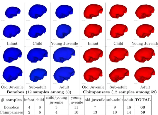
As part of the collaborative project ARC 3D-Morphine, we used a set of en-docasts of 59 chimpanzees and 60 bonobos. The original skulls are from the collection of “Musée de l’Afrique centrale” in Tervuren, Belgium (curator: E. Gilissen). They represent wild-shot individuals with approximately equal num-bers of male and female. They have been scanned using a Siemens Somatom Esprit Spiral CT, with slice thickness between 0.33 and 0.50mm. The segmen-tation of the endocasts using itkSNAP [18] leads to surface meshes, as shown in Fig. 5. These surfaces have been rigidly co-registered using gmmreg [6].
The analysis of the permanent teeth development of the skulls provides an estimate of the age of the death of the samples, which we call here “dental age”. It has been observed in [7] that the sequences teeth emergence in bonobos and chimpanzees are essentially identical. Each skull is therefore associated to one the 6 dental ages defined in [14]: infant, child, young juvenile, old juvenile, sub-adult and sub-adult. To refine the classification, some skulls have been associated the intermediate class ‘child/young juvenile’ by the experts. Age distribution is shown in Fig 5.
Infant Child Young Juvenile
Old Juvenile Sub-adult Adult
Infant Child Young Juvenile
Old Juvenile Sub-adult Adult Bonobos (12 samples among 60) Chimpanzees (12 samples among 59) # samples infant child child/young
juvenile
young
juvenile old juvenile sub-adult adult TOTAL
Bonobos 4 8 3 11 7 9 18 60
Chimpanzees 2 6 4 10 13 10 14 59
Fig. 5.Samples of the original endocasts of both species (top) and their distribution according to their dental age (bottom)
3.2 Typical growth scenario estimation
Without loss of generality, we assume that each of the dental age lasts the same amount of time, namely 5 time steps. Therefore the time interval of in-terest has been divided into 30 time-steps and the endocasts are associated to the time-point ti = 5, 10, 15, 20, 25, 30 according to their dental age. The age
child/young juvenile has been associated to the time-point 13. We choose the smallest endocast within the child class as the baseline S0and associate it to the
time point t = 2. Then, we perform a temporal shape regression of the endocasts (independently for each species) with respect to the dental age by minimizing the cost function (2.1). We set the typical spatial interaction between currents λW = 20mm, the spatial scale of deformation consistency λχ = 50mm and the
trade-off between fidelity-to-data and regularity γχ = 10−4mm 2
(unit of time). The diameter of the endocasts are typically between 60 and 70mm.
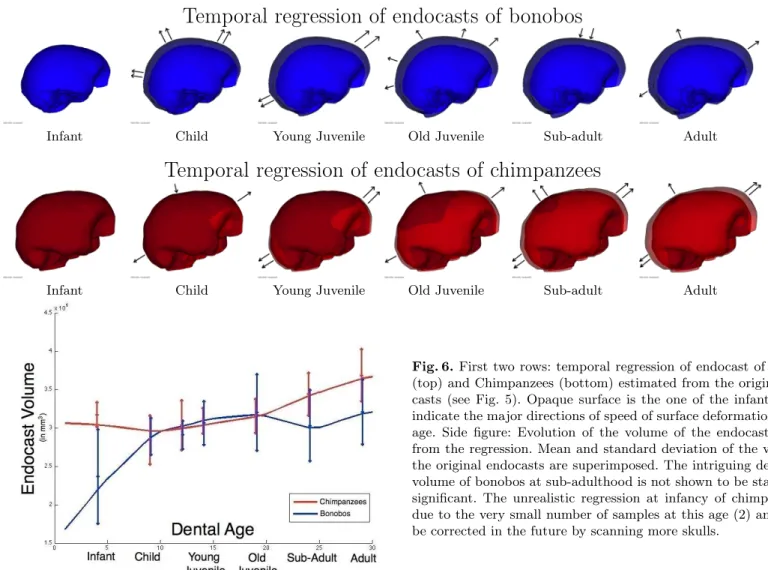
Results are shown in Fig. 6. The scenarios reveal that the endocast growth is not a simple scaling but involves non-linear and anisotropic effects. The most salient effect, besides the increase of volume, is an elongation along the poste-rior/anterior axis and a slight contraction along the superior/inferior axis. As a consequence, the geometry of the endocast, which is almost spherical at birth, becomes more and more ellipsoidal. These observations hold for both species,
although it seems that the chimpanzees endocasts have a strongest anisotropy and that this anisotropy increases faster in time. The subsequent spatiotemporal registration will measure these differences more precisely.
By contrast, the two growth scenarios seem to differ a lot at infancy and childhood. This difference is due to the little amount of data in infancy. The only two infant chimpanzees have a larger endocasts compared to both the infant bonobos and the children chimpanzees. To have a more relevant estimation of the growth in infancy, we expect to scan more infant chimpanzees skulls in the future. Note that in the next section we will not take the infancy data into account and will consider the growth scenarios starting at childhood.
We can deduce from the growth scenario an estimation of the evolution of the endocranial volume across ages, as shown in Fig. 6 (Note that we have not performed a regression of the volume but of the shapes). Besides the evolution in infancy, one intriguing feature is the apparent decrease of bonobos endocranial volume at sub-adulthood. This feature is also present in the endocranial volume distribution in the original endocasts (mean and standard deviation are shown in Fig. 6): the mean of the volume at sub-adulthood is smaller than the one of old juveniles. However, the Mann-Whitney U test gives a p-value of 0.47 when comparing the volume distribution of old juveniles and sub-adults: the median of the two distributions are not proved to be statistically different. The test run for every pair of consecutive distributions shows a significant increase of volume only between infancy and childhood for the bonobos (p-value: 9 10−3) and between
old-juvenility and sub-adulthood for the chimpanzees (p-value: 0.02).
3.3 Spatiotemporal registration between the growth scenarios We perform a spatiotemporal registration between the two growth scenar-ios starting at childhood for the reasons explained in the previous section. We consider the chimpanzee growth scenario as the reference scenario. The bonobo scenario is sampled every 2 time-steps. These samples play the role of the tar-get shapes. We set the scale of currents to λW = 20mm as for the regression
estimation. We run the registration for different set of parameters and pick the ones which enable to achieve the smallest discrepancy term in (2.2). This gives the consistency scale of the morphological deformation: λφ = 10mm, the
con-sistency scale of the time-warp λψ = 1 unit of time, morphological trade-off
γφ= 25 10−9mm2
and the temporal trade-off γψ = 4 10−9mm4
/(unit of time). The morphological deformation changes the shape of each frame of the chim-panzee growth as shown in Fig. 7a (this is the equivalent figure to the first and second row in Fig. 4a). It shows that, independently of the age, the bonobos endocast are rounder than the chimpanzees ones. The movie of this deformation clearly shows a twist at the anterior and posterior part of the endocast. This effect could be quantify, for instance by measuring the ratio between the elon-gation in the superior-inferior and the posterior-anterior direction. This shows how our analysis can be used to drive the search of relevant anatomical features, in contrast to methods like [1] which select the information a priori.
The graph of the estimated time-warp is shown in Fig. 7b. Its shows the ages of the bonobos match the chimpanzees ones. An important speed reduction of the growth of the bonobos with respect to the chimpanzees occurs between old-juvenility and sub-adulthood. The almost constant slope of the curve during this period of time indicates that the bonobos growth speed is 0.42 times that of the chimpanzees. The graph shows also that the bonobos seem to be slightly in advance with respect to the chimpanzees at childhood and that the delay of the bonobos growth at sub-adulthood seems to be reduced at adulthood.
4
Discussion and conclusion
The experiments on this set of endocasts showed that the proposed method-ology enables to detect, measure and compare growth patterns in a set of time-indexed shapes. The shape regression averaged the inter-individual variability and estimated a typical growth scenario for each species. The comparison of the growth scenarios using the spatiotemporal registration gave more insights into the “bonobos hypothesis”. The measure of the morphological differences based on non-linear 3D deformation allowed us to detect anisotropic variations, which can-not be seen by the analysis of some simple geometrical features like the volume for instance. The non-linearity of the time-warp allowed us to detect not only the expected developmental delay of the bonobos but also more subtle effects like the developmental advance of bonobos at childhood or the delay reduc-tion at adulthood. If we assume an ancestor relareduc-tionship between both species, this measure suggests that the analysis of heterochrony cannot be reduced to a black-and-white decision between paedomorphosis and peramorphosis [9].
This analysis is based on a generic methodology which reduces the depen-dence on expert choices like the locations of landmarks. The anatomical features of interest are not selected a priori but appears as the result of the analysis. Fu-ture work should focus on the extraction and quantification of the feaFu-tures which seems the most discriminative, like the “roundness” of the endocast for instance. The method depends on exactly 7 parameters, which have a physical or statis-tical interpretation [2]. The parameters of the spatiotemporal registration have been set so that it reduces the dissimilarity between the deformed source and the target. Note that due to the modeling assumptions, there may not be any set of parameters which achieves a perfect data fit (i.e. zero residuals). We proposed here to measure the inter-species growth differences using the estimated growth scenarios. This has some drawbacks: one does not account for the fact that one has a different number of samples at each age and this approach is not symmetric as we chose the chimpanzee as the reference species. To overcome these issues, we will use the unbiased atlas construction scheme of [3] in the future. One also needs to investigate the variability of the results with respect to the parameters and the samples. For instance, bootstrap procedure can be used to estimate a confidence interval around the growth scenarios.
Acknowledgments We thank B. Combès for data pre-processing, Wim Van Neer as the former curator of the ‘Musée de l’Afrique Centrale’ at Tervuren, G. Subsol
and S. Prima for their active role in the project 3D-Morphine and G. Gerig for his insightful comments. We thank the anonymous reviewers for their relevant sug-gestions. This work has been partly funded by the INRIA ARC 3D-Morphine, the European IP project Health-e-child (IST-2004-027749) and Microsoft Research.
References
1. Bookstein, F.: Morphometric tools for landmark data: geometry and biology. Cam-bridge University Press (1991)
2. Durrleman, S.: Statistical models of currents for measuring the variability of anatomical curves, surfaces and their evolution. Thèse de sciences (phd thesis), Université de Nice-Sophia Antipolis (2010)
3. Durrleman, S., Pennec, X., Trouvé, A., Gerig, G., Ayache, N.: Spatiotemporal atlas estimation for developmental delay detection in longitudinal datasets. In: Proc. of MICCAI 2009. LNCS, vol. 5761, pp. 297–304. Springer
4. Durrleman, S., Pennec, X., Trouvé, A., Thompson, P., Ayache, N.: Inferring brain variability from diffeomorphic deformations of currents: an integrative approach. Medical Image Analysis 12/5(12), 626–637 (2008)
5. Glaunès, J.: Transport par difféomorphismes de points, de mesures et de courants pour la comparaison de formes et l’anatomie numérique. Ph.D. thesis, Université Paris 13, http://cis.jhu.edu/ joan/TheseGlaunes.pdf (September 2005)
6. Jian, B., Vemuri, B.C.: A robust algorithm for point set registration using mixture of Gaussians. In: Proc. of ICCV’05. pp. 1246–1251. gmmreg.googlecode.com 7. Kinzey, W.G.: The dentition of the pygmy chimpanzee, Pan paniscus, pp. 65–88.
Plenum (New York) (1984)
8. Kuroda, S.: Developmental retardation and behavioural characteristics of pygmy chimpanzees, pp. 184–193. Harvard University Press (1989)
9. Lieberman, D.E., Carlo, J., de León, M.P., Zollikofer, C.P.: A geometric morphome-tric analysis of heterochrony in the cranium of chimpanzees and bonobos. Journal of Human Evolution 52, 647–662 (2007)
10. Macrini, T.E., Rowe, T., VandeBerg, J.L.: Cranial endocasts from a growth series of Monodelphis domestica (Didelphidae, Marsupiala): A study of individual and ontogenetic variation. Journal of Morphology 268, 844–865 (2007)
11. Neubauer, S., Gunz, P., Hublin, J.J.: The pattern of endocranial ontogenetic shape changes in humans. Journal of Anatomy 215, 240–255 (2009)
12. Radinsky, L.: Brains of early carnivores. Paleobiology 3, 333–349 (1977)
13. Schwarz, E.: Das Vorkommen des Schimpanzen auf then linked Kongo-Ufer. Rev. Zool. Bot. Afr. 16, 425–426 (1929)
14. Shea, B.: Heterochrony in human evolution: The case for neoteny reconsidered. Yearb. Phys. Anthropol. 32, 69–101 (1989)
15. Vaillant, M., Glaunès, J.: Surface matching via currents. In: Proc. of IPMI. LNCS, vol. 3565, pp. 381–392. Springer (2005)
16. de Waal, F.B.M.: Bonobo sex and society. Scientific American 272, 82–88 (1995) 17. Won, Y., Hey, J.: Divergence population genetics of chimpanzees. Mol. Biol. Evol.
22, 297–307 (2005)
18. Yushkevich, P.A., Piven, J., Cody Hazlett, H., Gimpel Smith, R., Ho, S., Gee, J.C., Gerig, G.: User-guided 3D active contour segmentation of anatomical struc-tures: Significantly improved efficiency and reliability. Neuroimage 31(3), 1116– 1128 (2006)
Temporal regression of endocasts of bonobos
Infant Child Young Juvenile Old Juvenile Sub-adult Adult
Temporal regression of endocasts of chimpanzees
Infant Child Young Juvenile Old Juvenile Sub-adult Adult
Fig. 6.First two rows: temporal regression of endocast of Bonobos (top) and Chimpanzees (bottom) estimated from the original endo-casts (see Fig. 5). Opaque surface is the one of the infant. Arrows indicate the major directions of speed of surface deformation at each age. Side figure: Evolution of the volume of the endocast inferred from the regression. Mean and standard deviation of the volume of the original endocasts are superimposed. The intriguing decrease of volume of bonobos at sub-adulthood is not shown to be statistically significant. The unrealistic regression at infancy of chimpanzees is due to the very small number of samples at this age (2) and should be corrected in the future by scanning more skulls.
Child Old Juvenile Adult
a- Morphological Deformation
The morphological deformation is applied to the chimpanzees endocasts at 3 ages. Left column: the endocasts from the chimpanzees growth scenario. Right: the de-formed endocasts. Middle: an intermediate deformation. This shows that, on aver-age, the endocast of a chimpanzee is more elongated and less round than the one of a bonobo (more clearly visible on the movie of the deformation). Note that the deformed endocasts do not match the ones of the bonobo growth at the same age, but at the age given by the correspondence graph shown in
b-The dashed black line represents the non dynamical changes axis (x = y). When the time-warp (magenta curve) is above (resp. below) the dashed line, bonobo growth is in advance (resp. delayed) w.r.t. the chimpanzee growth. Slope greater than 1 (resp. smaller than 1) indicates that the bonobo growth accelerates (resp. slows down) w.r.t. to the chimpanzee growth.
b- Time Warp
Graph of time-warp showing that the bonobos devel-opment is in advance with respect to the chimpanzees one at childhood and then that it drastically slows down during juvenility (almost linearly by a factor 0.42 between old-juvenility and sub-adulthood). This delay seems to decrease at adulthood.