Causal impact of masks, policies, behavior on early covid-19 pandemic in the U.S.

(1)

Causal impact of masks, policies, behavior

on early covid-19 pandemic in the U.S.

The MIT Faculty has made this article openly available. Please share

how this access benefits you. Your story matters.

Citation

Chernozhukov, Victor et al. "Causal impact of masks, policies,

behavior on early covid-19 pandemic in the U.S." Journal of

Econometrics 220, 1 (January 2021): 23-62 © 2020 The Author(s)

As Published

http://dx.doi.org/10.1016/j.jeconom.2020.09.003

Publisher

Elsevier BV

Version

Final published version

Citable link

https://hdl.handle.net/1721.1/128951

Terms of Use

Creative Commons Attribution 4.0 International license

(2)

Contents lists available atScienceDirect

Journal of Econometrics

journal homepage:www.elsevier.com/locate/jeconom

Causal impact of masks, policies, behavior on early covid-19

pandemic in the U.S.

Victor Chernozhukov

a

_{, Hiroyuki Kasahara}

b,∗

, Paul Schrimpf

b

a_{Department of Economics and Center for Statistics and Data Science, MIT, MA 02139, United States of America} b_{Vancouver School of Economics, UBC, 6000 Iona Drive, Vancouver, BC, Canada}

a r t i c l e i n f o

Article history:

Received 3 July 2020

Received in revised form 3 July 2020 Accepted 15 September 2020 Available online 17 October 2020

Keywords: Covid-19 Causal impact Masks Policies Behavior a b s t r a c t

The paper evaluates the dynamic impact of various policies adopted by US states on the growth rates of confirmed Covid-19 cases and deaths as well as social distancing be-havior measured by Google Mobility Reports, where we take into consideration people’s voluntarily behavioral response to new information of transmission risks in a causal structural model framework. Our analysis finds that both policies and information on transmission risks are important determinants of Covid-19 cases and deaths and shows that a change in policies explains a large fraction of observed changes in social distancing behavior. Our main counterfactual experiments suggest that nationally mandating face masks for employees early in the pandemic could have reduced the weekly growth rate of cases and deaths by more than 10 percentage points in late April and could have led to as much as 19 to 47 percent less deaths nationally by the end of May, which roughly translates into 19 to 47 thousand saved lives. We also find that, without stay-at-home orders, cases would have been larger by 6 to 63 percent and without business closures, cases would have been larger by 17 to 78 percent. We find considerable uncertainty over the effects of school closures due to lack of cross-sectional variation; we could not robustly rule out either large or small effects. Overall, substantial declines in growth rates are attributable to private behavioral response, but policies played an important role as well. We also carry out sensitivity analyses to find neighborhoods of the models under which the results hold robustly: the results on mask policies appear to be much more robust than the results on business closures and stay-at-home orders. Finally, we stress that our study is observational and therefore should be interpreted with great caution. From a completely agnostic point of view, our findings uncover predictive effects (association) of observed policies and behavioral changes on future health outcomes, controlling for informational and other confounding variables.

1. Introduction

Accumulating evidence suggests that various policies in the US have reduced social interactions and slowed down the growth of Covid-19 infections.1 An important outstanding issue, however, is how much of the observed slow down in the spread is attributable to the effect of policies as opposed to a voluntarily change in people’s behavior out of fear of being infected. This question is critical for evaluating the effectiveness of restrictive policies in the US relative to an

∗ _{Corresponding author.}

E-mail addresses: vchern@mit.edu(V. Chernozhukov),hkasahar@mail.ubc.ca(H. Kasahara),schrimpf@mail.ubc.ca(P. Schrimpf).

1 _See_{Courtemanche et al.}₍₂₀₂₀_),_{Hsiang et al.}₍₂₀₂₀_),_{Pei et al.}₍₂₀₂₀_),_{Abouk and Heydari}₍₂₀₂₀_{), and}_{Wright et al.}₍₂₀₂₀_).

https://doi.org/10.1016/j.jeconom.2020.09.003

(3)

alternative policy of just providing recommendations and information such as the one adopted by Sweden. More generally, understanding people’s dynamic behavioral response to policies and information is indispensable for properly evaluating the effect of policies on the spread of Covid-19.

This paper quantitatively assesses the impact of various policies adopted by US states on the spread of Covid-19, such as non-essential business closure and mandatory face masks, paying particular attention to how people adjust their behavior in response to policies as well as new information on cases and deaths.

We present a conceptual framework that spells out the causal structure on how the Covid-19 spread is dynamically determined by policies and human behavior. Our approach explicitly recognizes that policies not only directly affect the spread of Covid-19 (e.g., mask requirement) but also indirectly affect its spread by changing people’s behavior (e.g., stay-at-home order). It also recognizes that people react to new information on Covid-19 cases and deaths and voluntarily adjust their behavior (e.g., voluntary social distancing and hand washing) even without any policy in place. Our causal model provides a framework to quantitatively decompose the growth of Covid-19 cases and deaths into three components: (1) direct policy effect, (2) policy effect through behavior, and (3) direct behavior effect in response to new information. Guided by the causal model, our empirical analysis examines how the weekly growth rates of confirmed Covid-19 cases and deaths are determined by (the lags of) policies and behavior using US state-level data. To examine how policies and information affect people’s behavior, we also regress social distancing measures on policy and information variables. Our regression specification for case and death growths is explicitly guided by a SIR model although our causal approach does not hinge on the validity of a SIR model.

As policy variables, we consider mandatory face masks for employees in public businesses, stay-at-home orders (or shelter-in-place orders), closure of K-12 schools, closure of restaurants except take out, closure of movie theaters, and closure of non-essential businesses. Our behavior variables are four mobility measures that capture the intensity of visits to ‘‘transit’’, ‘‘grocery’’, ‘‘retail’’, and ‘‘workplaces’’ from Google Mobility Reports. We take the lagged growth rate of cases and deaths and the log of lagged cases and deaths at both the state-level and the national-level as our measures of information on infection risks that affects people’s behavior. We also consider the growth rate of tests, month dummies, and state-level characteristics (e.g., population size and total area) as confounders that have to be controlled for in order to identify the causal relationship between policy/behavior and the growth rate of cases and deaths.

Our key findings from regression analysis are as follows. We find that both policies and information on past cases and deaths are important determinants of people’s social distancing behavior, where policy effects explain more than 50% of the observed decline in the four behavior variables.2Our estimates suggest that there are both large policy effects and large behavioral effects on the growth of cases and deaths. Except for mandatory masks, the effect of policies on cases and deaths is indirectly materialized through their impact on behavior; the effect of mandatory mask policy is direct without affecting behavior.

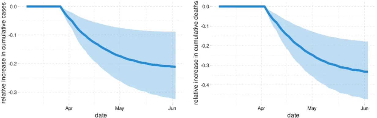
Using the estimated model, we evaluate the dynamic impact of the following three counterfactual policies on Covid-19 cases and deaths: (1) mandating face masks, (2) allowing all businesses to open, and (3) not implementing a stay-at-home order. The counterfactual experiments show a large impact of those policies on the number of cases and deaths. They also highlight the importance of voluntary behavioral response to infection risks when evaluating the dynamic policy effects. Our estimates imply that nationally implementing mandatory face masks for employees in public businesses on March 14th would have reduced the growth rate of cases and that of deaths by approximately 10 percentage points in late April. As shown inFig. 1, this leads to reductions of 21% and 34% in cumulative reported cases and deaths, respectively, by the end of May with 90 percent confidence intervals of

[

9

,

32

]

% and

[

19

,

47

]

%, which roughly implies that 34 thousand lives could have been saved. This finding is significant: given this potentially large benefit of reducing the spread of Covid-19, mandating masks is an attractive policy instrument especially because it involves relatively little economic disruption. These estimates contribute to the ongoing efforts towards designing approaches to minimize risks from reopening (Stock,

2020b).

Fig. 2illustrates how never closing any businesses (no movie theater closure, no non-essential business closure, and no

closure of restaurants except take-out) could have affected cases and deaths. We estimate that business shutdowns have roughly the same impact on growth rates as mask mandates, albeit with more uncertainty. The point estimates indicate that keeping all businesses open could have increased cumulative cases and deaths by 40% at the end of May (with 90 percent confidence intervals of

[

17

,

78

]

% for cases and

[

1

,

97

]

% for deaths).

Fig. 3shows that stay-at-home orders had effects of similar magnitude as business closures. No stay-at-home orders

could have led to 37% more cases by the start of June with a 90 percent confidence interval given by 6% to 63%. The estimated effect of no stay-at-home orders on deaths is a slightly smaller with a 90 percent confidence interval of

−

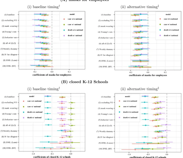
7% to 50%.

We also conducted sensitivity analysis with respect to changes to our regression specification, sample selection, methodology, and assumptions about delays between policy changes and changes in recorded cases. In particular, we examined whether certain effect sizes can be ruled out by various more flexible models or by using alternative timing assumptions that define forward growth rates. The impact of mask mandates is more robustly and more precisely estimated than that of business closure policies or stay-at-home orders, and an undesirable effect of increasing the weekly

2 _{The behavior accounts for the other half. This is in line with theoretical study by}_{Gitmez et al.}₍₂₀₂₀_{) that investigates the role of private}

(4)

Fig. 1. Relative cumulative effect on confirmed cases and fatalities of nationally mandating masks for employees on March 14th in the US. This figure shows the estimated relative change in cumulative cases and deaths if all states had mandated masks on March 14th. The thick blue line is the estimated change in cumulative cases or deaths relative to the observed number of cases or deaths. The shaded region is a pointwise 90% confidence band.

Fig. 2. Relative cumulative effect of no business closure policies on cases and fatalities in the US. This figure shows the estimated relative change in cases and deaths if no states had ever implemented any business closure policies. The thick blue line is the estimated change in cumulative cases or deaths relative to the observed number of cumulative cases or deaths. The shaded region is a pointwise 90% confidence band.

death growth by 5 percentage points is ruled out by all of the models we consider.3 This is largely due to the greater variation in the timing of mask mandates across states. The findings of shelter-in-place and business closures policies are considerably less robust. For example, for stay-at-home mandates, models with alternative timing and richer specification for information set suggested smaller effects. Albeit after application of machine learning tools to reduce dimensionality, the range of effects

[

0

,

0

.

15

]

could not be ruled out. A similar wide range of effects could not be ruled out for business closures.

We also examine the impact of school closures. Unfortunately, there is very little variation across states in the timing of school closures. Across robustness specifications, we obtain point estimates of the effect of school closures as low as 0 and as high as -0.6. In particular, we find that the results are sensitive to whether the number of past national cases/deaths is included in a specification or not. This highlights the uncertainty regarding the impact of some policies versus private behavioral responses to information.

A growing number of other papers have examined the link between non-pharmaceutical interventions and Covid-19 cases.4Hsiang et al.(2020) estimate the effect of policies on the growth rate of cases using data from the United States, China, Iran, Italy, France, and South Korea. In the United States, they find that the combined effect of all policies they consider on the growth rate is

−

0

.

347 (0

.

061).Courtemanche et al.(2020) use US county level data to analyze the effect of interventions on case growth rates. They find that the combination of policies they study reduced growth rates by 9.1

3 _{This null hypothesis can be generated by looking at the meta-evidence from RCTs on the efficacy of masks in preventing other respiratory}

cold-like deceases. Falsely rejecting this null is costly in terms of potential loss of life, and so it is a reasonable null choice for the mask policy from decision-theoretic point of view.

4 _{We refer the reader to}_{Avery et al.}₍₂₀₂₀_{) for a comprehensive review of a larger body of work researching Covid-19; here we focus on few}

(5)

Fig. 3. Relative cumulative effect of not implementing stay-at-home order on cases and fatalities in the US. This figure shows the estimated relative change in cases and deaths if no states had ever issued stay at home orders. The thick blue line is the estimated change in cumulative cases or deaths relative to the observed number of cumulative cases or deaths. The shaded region is a point wise 90% confidence band.

percentage points 16–20 days after implementation, out of which 5.9 percentage points are attributable to shelter in place orders. BothHsiang et al.(2020) andCourtemanche et al.(2020) adopt a reduced-form approach to estimate the total policy effect on case growth without using any social distancing behavior measures.5

Existing evidence for the impact of social distancing policies on behavior in the US is mixed.Abouk and Heydari(2020) employ a difference-in-differences methodology to find that statewide stay-at-home orders have strong causal impacts on reducing social interactions. In contrast, using data from Google Mobility Reports,Maloney and Taskin(2020) find that the increase in social distancing is largely voluntary and driven by information.6 Another study byGupta et al.(2020) also found little evidence that stay-at-home mandates induced distancing by using mobility measures from PlaceIQ and SafeGraph. Using data from SafeGraph,Andersen(2020) shows that there has been substantial voluntary social distancing but also provide evidence that mandatory measures such as stay-at-home orders have been effective at reducing the frequency of visits outside of one’s home.

Pei et al.(2020) use county-level observations of reported infections and deaths in conjunction with mobility data from

SafeGraph to conduct simulation of implementing all policies 1–2 weeks earlier and found that it would have resulted in reducing the number of cases and deaths by more than half. However, their study does not explicitly analyze how policies are related to the effective reproduction numbers.

Epidemiologists use model simulations to predict how cases and deaths evolve for the purpose of policy recommenda-tion. As reviewed byAvery et al.(2020), there exists substantial uncertainty about the values of key epidemiological parameters (see alsoAtkeson, 2020a; Stock, 2020a). Simulations are often done under strong assumptions about the impact of social distancing policies without connecting to the relevant data (e.g.,Ferguson et al.,2020). Furthermore, simulated models do not take into account that people may limit their contact with other people in response to higher transmission risks.7When such a voluntary behavioral response is ignored, simulations would necessarily exhibit exponential spread and over-predict cases and deaths. In contrast, as cases and deaths rise, a voluntary behavioral response may possibly reduce the effective reproduction number below 1, potentially preventing exponential spread. Our counterfactual experiments illustrate the importance of this voluntary behavioral change.

Whether wearing masks in public place should be mandatory or not has been one of the most contested policy issues with health authorities of different countries providing contradictory recommendations. Reviewing evidence,Greenhalgh

et al.(2020) recognize that there is no randomized controlled trial evidence for the effectiveness of face masks, but they

state ‘‘indirect evidence exists to support the argument for the public wearing masks in the Covid-19 pandemic’’.8Howard

et al.(2020) also review available medical evidence and conclude that ‘‘mask wearing reduces the transmissibility per

contact by reducing transmission of infected droplets in both laboratory and clinical contexts’’. The laboratory findings

inHou et al.(2020) suggest that the nasal cavity may be the initial site of infection followed by aspiration to the lung,

supporting the argument ‘‘for the widespread use of masks to prevent aerosol, large droplet, and/or mechanical exposure

5 _{Using a synthetic control approach,}_Cho₍₂₀₂₀_{) finds that the cases would have been lower by 75 percent had Sweden adopted stricter lockdown}

policies.

6 _{Specifically, they find that of the 60 percentage point drop in workplace intensity, 40 percentage points can be explained by changes in}

information as proxied by case numbers, while roughly 8 percentage points can be explained by policy changes.

7 _See_Atkeson₍_2020b_{) and}_Stock₍_2020a_{) for the implications of the SIR model for Covid-19 in the US.}_{Fernández-Villaverde and Jones}₍₂₀₂₀₎

estimate a SIRD model in which time-varying reproduction numbers depend on the daily deaths to capture feedback from daily deaths to future behavior and infections.

8 _{The virus remains viable in the air for several hours, for which surgical masks may be effective. Also, a substantial fraction of individual who}

(6)

to the nasal passages’’.He et al.(2020) examined temporal patterns of viral shedding in COVID-19 patients and found the highest viral load at the time of symptom onset; this suggests that a significant portion of transmission may have occurred before symptom onset and that universal face masks may be an effective control measure to reduce transmission.9Ollila

et al. (2020) provide a meta-analysis of randomized controlled trials of non-surgical face masks in preventing viral

respiratory infections in non-hospital and non-household settings, finding that face masks decreased infections across all five studies they reviewed.10

Given the lack of experimental evidence on the effect of masks in the context of COVID-19, conducting observational studies is useful and important. To the best of our knowledge, our paper is the first empirical study that shows the effectiveness of mask mandates on reducing the spread of Covid-19 by analyzing the US state-level data. This finding corroborates and is complementary to the medical observational evidence inHoward et al.(2020). Analyzing mitigation measures in New York, Wuhan, and Italy,Zhang et al.(2020b) conclude that mandatory face coverings substantially reduced infections.Abaluck et al.(2020) find that the growth rates of cases and of deaths in countries with pre-existing norms that sick people should wear masks are lower by 8 to 10% than those rates in countries with no pre-existing mask norms.11 The Institute for Health Metrics and Evaluation at the University of Washington assesses that, if 95% of the people in the US were to start wearing masks from early August of 2020, 66,000 lives would be saved by December 2020 (IHME, 2020), which is largely consistent with our results. Our finding is also independently corroborated by a completely different causal methodology based on synthetic control using German data inMitze et al.(2020).12

Our empirical results contribute to informing the economic-epidemiological models that combine economic models with variants of SIR models to evaluate the efficiency of various economic policies aimed at the gradual ‘‘reopening’’ of various sectors of economy.13For example, the estimated effects of masks, stay-home mandates, and various other policies on behavior, and of behavior on infection can serve as useful inputs and validation checks in the calibrated macro, sectoral, and micro models (see, e.g.,Alvarez et al.,2020;Baqaee et al.,2020;Fernández-Villaverde and Jones,2020;Acemoglu et al.,

2020;Keppo et al.,2020;McAdams,2020and references therein). Furthermore, the causal framework developed in this

paper could be applicable, with appropriate extensions, to the impact of policies on economic outcomes replacing health outcomes (see, e.g.,Chetty et al.,2020;Coibion et al.,2020).

Finally, our causal model is framed using the language of structural equations models and causal diagrams of econometrics (Wright,1928;Haavelmo,1944;Tinbergen,1940;Wold,1954;Pearl,1995) and genetics (Wright,1923),14 with natural unfolding potential/structural outcomes representation (Rubin, 1974; Tinbergen, 1930; Neyman, 1925;

Imbens and Rubin,2015). The work on causal graphs has been modernized and developed by Pearl(1995),Greenland

et al.(1999), Pearl(2009), Pearl and Mackenzie (2018) and many others (e.g.,Pearl and Mackenzie,2018; White and

Chalak,2009;Robins et al.,2020;Peters et al.,2017;Bareinboim et al.,2020;Hernán and Robins,2020), with applications

in computer science, genetics, epidemiology, and econometrics (see, e.g.,Heckman and Pinto,2013; Hünermund and

Bareinboim,2019;White and Chalak,2009for applications in econometrics). The particular causal diagram we use has

several ‘‘mediation’’ components, where variables affect outcomes directly and indirectly through other variables called mediators; these structures go back at least toWright(1923, see Figure 6); see, e.g.,Baron and Kenny(1986),Hines et al.

(2020),Robins et al.(2020) for modern treatments.

2. The causal model for the effect of policies, behavior, and information on growth of infection

2.1. The causal model and its structural equation form

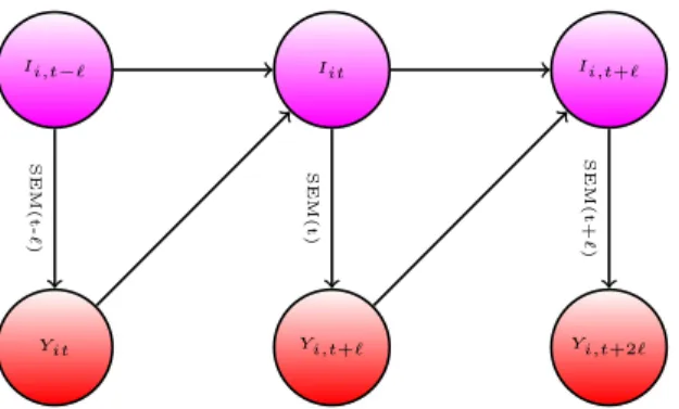
We introduce our approach through the Wright-style causal diagram shown in Fig. 4. The diagram describes how policies, behavior, and information interact together:

•

The forward health outcome, Yi,t+ℓ, is determined last, after all other variables have been determined;

•

The adopted policies, Pit, affect health outcome Yi,t+_ℓeither directly, or indirectly by altering human behavior Bit;

9 _{Lee et al.}₍_2020a_{) find evidence that viral loads in asymptomatic patients are similar to those in symptomatic patients. Aerosol transmission}

of viruses may occur through aerosols particles released during breathing and speaking by asymptomatic infected individuals; masks reduce such airborne transmission (Prather et al.,2020).Anfinrud et al.(2020) provide visual evidence of speech-generated droplet as well as the effectiveness of cloth masks to reduce the emission of droplets.Chu et al.(2020) conduct a meta-analysis of observational studies on transmission of the viruses that cause COVID-19 and related diseases and find the effectiveness of mask use for reducing transmission.

10 _{Whether wearing masks creates a false sense of security and leads to decrease in social distancing is also a hotly debated topic. A randomized}

field experiment in Berlin, Germany, conducted bySeres et al.(2020) finds that wearing masks actually increases social distancing, providing no evidence that mandatory masks leads to decrease in social distancing.

11 _{Miyazawa and Kaneko}₍₂₀₂₀_{) find that country’s COVID-19 death rates are negatively associated with mask wearing rates.} 12 _{Our study was first released in ArXiv on May 28, 2020 whereas}_{Mitze et al.}₍₂₀₂₀_{) was released at SSRN on June 8, 2020.}

13 _Adda₍₂₀₁₆_{) analyzes the effect of policies reducing interpersonal contacts such as school closures or the closure of public transportation}

networks on the spread of influenza, gastroenteritis, and chickenpox using high frequency data from France.

14 _{The father and son, P. Wright (economist) and S. Wright (geneticist) collaborated to develop structural equation models and causal path diagrams;}

P. Wright’s key work represented supply–demand system as a directed acyclical graph and established its identification using exclusion restrictions on instrumental variables. We view our work as following this classical tradition.

(7)

Fig. 4. S. & P. Wright type causal path diagram for our model.

•

Information variables, Iit, such as lagged values of outcomes can affect human behavior and policies, as well as

outcomes;

•

The confounding factors Wit, which vary across states and time, affect all other variables.

The index i denotes observational unit, the state, and t and t

+

ℓ

denotes the time, where

ℓ

is a positive integer that represents the time lag between infection and case confirmation or death.

Our main outcomes of interest are the growth rates in Covid-19 cases and deaths, behavioral variables include proportion of time spent in transit, shopping, and workplaces, policy variables include mask mandates, stay-at-home orders, and school and business closures, and the information variables include lagged values of outcome. We provide a detailed description of these variables and their timing in the next section.

The causal structure allows for the effect of the policy to be either direct or indirect — through behavior or through dynamics; all of these effects are not mutually exclusive. The structure also allows for changes in behavior to be brought by change in policies and information. These are all realistic properties that we expect from the contextual knowledge of the problem. Policies such as closures of schools, non-essential business, and restaurants alter and constrain behavior in strong ways. In contrast, policies such as mandating employees to wear masks can potentially affect the Covid-19 transmission directly. The information variables, such as recent growth in the number of cases, can cause people to spend more time at home, regardless of adopted state policies; these changes in behavior in turn affect the transmission of Covid-19. Importantly, policies can have the informational content as well, guiding behavior rather than constraining it.

The causal ordering induced by this directed acyclical graph is determined by the following timing sequence: (1) information and confounders get determined at t,

(2) policies are set in place, given information and confounders at t; (3) behavior is realized, given policies, information, and confounders at t;

(4) outcomes get realized at t

+

ℓ

given policies, behavior, information, and confounders.

The model also allows for direct dynamic effects of information variables on the outcome through autoregressive structures that capture persistence in growth patterns. As highlighted below, realized outcomes may become new information for future periods, inducing dynamics over multiple periods.

Our quantitative model for causal structure in Fig. 4is given by the following econometric structural (or potential) outcomes model: Yi,t+ℓ(b

,

p

, ι

)

:=

α

′ b

+

π

′p

+

µ

′

ι

+

δ

_Y′Wit

+

ε

yit

,

Bit(p

, ι

)

:=

β

′p

+

γ

′

ι

+

δ

′BWit

+

ε

itb

,

(SO)

which is a collection of functional relations with stochastic shocks, decomposed into observable part

δ

′

W and unob-servable part

ε

. The terms

ε

y_it and

ε

b

itare the centered stochastic shocks that obey the orthogonality restrictions posed

below.

The policies can be modeled via a linear form as well, Pit(

ι

)

:=

η

′

ι

+

δ

′_PWit

+

ε

pit

,

(P)

although linearity is not critical.15

15 _{Under some additional independence conditions, this can be replaced by an arbitrary non-additive function P}

it(ι)=p(ι,Wit, εitp), such that the

(8)

Fig. 5. Diagram for Information Dynamics in SEM.

The exogeneity restrictions on the stochastic shocks are as follows:

ε

y it

⊥

(

ε

b it

, ε

p it

,

Wit

,

Iit)

,

ε

b it

⊥

(

ε

p it

,

Wit

,

Iit)

,

ε

p it

⊥

(Wit

,

Iit)

,

(E)

where we say that V

⊥

U if EVU

=

0.16This is a standard way of representing restrictions on errors in structural equation modeling in econometrics.17

The observed variables are generated by setting

ι =

Iitand propagating the system from the last equation to the first: Yi,t+ℓ

:=

Yi,t+ℓ(Bit

,

Pit

,

Iit)

,

Bit

:=

Bit(Pit

,

Iit)

,

Pit

:=

Pit(Iit)

.

(O)

The specification of the model above grasps one-period responses. The dynamics over multiple periods will be induced by the evolution of information variables, which include time, lagged and integrated values of outcome18:

Iit

:=

It(Yit

,

Ii,t−_ℓ)

:=

(

g(t)

,

Yit

,

⌊t/ℓ⌋

∑

m=0 Yi,t−_ℓm

)

′ (I)

for each t

∈ {

0

,

1

, . . . ,

T

}

, where g is deterministic function of time, e.g., month indicators, assuming that the log of new cases at time t

≤

0 is zero, for notational convenience.19In this structure, people respond to both global information, captured by a function of time such as month dummies, and local information sources, captured by the local growth rate and the total number of cases. The local information also captures the persistence of the growth rate process. We model the reaction of people’s behavior via the term

γ

′

It in the behavior equation. The lagged values of behavior variable may

be also included in the information set, but we postpone this discussion after the main empirical results are presented. With any structure of this form, realized outcomes may become new information for future periods, inducing a dynamical system over multiple periods. We show the resulting dynamical system in a diagram ofFig. 5. Specification of this system is useful for studying delayed effects of policies and behaviors and in considering the counterfactual policy analysis.

Next we combine the above parts together with an appropriate initialization to give a formal definition of the model we use.

Structural Equations Model (SEM). Let i

∈ {

1

, . . . ,

N

}

denote the observational unit, t be the time periods, and

ℓ

be the time delay. (1) For each i and t

≤ −

ℓ

, the confounder, information, behavior, and policy variables

16 _{An alternative useful starting point is to impose the Rosenbaum–Rubin type unconfoundedness condition:} Yi,t+ℓ(·, ·, ·) y (Pit,Bit,Iit)|Wit, Bit(·, ·) y (Pit,Iit)|Wit,Pit(·) y Iit|Wit,

which imply, with treating stochastic errors as independent additive components, the orthogonal conditions stated above. The same unconfoundedness restrictions can be formulated using formal causal DAGs, and also imply orthogonality restrictions stated above, once stochastic errors are modeled as independent additive components.

17 _{The structural equations of this form are connected to triangular structural equation models, appearing in microeconometrics and}

macroeconometrics (SVARs), going back to the work ofStrotz and Wold(1960).

18 _{Our empirical analysis also considers a specification in which information variables include lagged national cases/deaths as well as lagged}

behavior variables.

19 _{The general formula for I}

i,t−1is Si,t,ℓ+∑⌊t/ℓ⌋

(9)

Wit

,

Iit

,

Bit

,

Pitare determined outside of the model, and the outcome variable Yi,t+_ℓis determined by factors outside

of the model for t

≤

0. (2) For each i and t

≥ −

ℓ

, confounders Witare determined by factors outside of the model,

and information variables Iitare determined by (I); policy variables Pitare determined by setting

ι =

Iitin (P) with

a realized stochastic shock

ε

_itp that obeys the exogeneity condition (E); behavior variables Bit are determined by

setting

ι =

Iitand p

=

Pit in (SO) with a shock

ε

b_itthat obeys (E); finally, the outcome Yi,t+ℓis realized by setting

ι =

Iit, p

=

Pit, and b

=

Bitin (SO) with a shock

ε

y

itthat obeys (E).

2.2. Main testable implication, identification, parameter estimation

The system above together with orthogonality restrictions(E)implies the following collection of projection equations for realized variables:

Yi,t+_ℓ

=

α

′ Bit

+

π

′ Pit

+

µ

′ Iit

+

δ

′ YWit

+

ε

ity

,

ε

y it

⊥

Bit

,

Pit

,

Iit

,

Wit (BPI

→

Y) Bit

=

β

′Pit

+

γ

′Iit

+

δ

B′Wit

+

ε

bit

,

ε

b it

⊥

Pit

,

Iit

,

Wit (PI

→

B) Pit

=

η

′ Iit

+

δ

′ PWit

+

ε

p it

,

ε

p it

⊥

Iit

,

Wit (I

→

P) Yi,t+ℓ

=

(

α

′

β

′

+

π

′)Pit

+

(

α

′

γ

′

+

µ

′)Iit

+

δ

¯

′ Wit

+ ¯

ε

it

,

ε

¯

it

⊥

Pit

,

Iit

,

Wit

.

(PI

→

Y)

Therefore the projection equation:

Yi,t+_ℓ

=

a ′ Pit

+

b ′ Iit

+

δ

˜

′ Wit

+ ¯

ε

it

, ¯ε

it

⊥

Pit

,

Iit

,

Wit

.

(Y

∼

PI) should obey: a′

=

(

α

′

β

′

+

π

′) andb′

=

(

α

′

γ

′

+

µ

′)

.

(TR) Without any exclusion restrictions, this equality is just a decomposition of total effects into direct and indirect components and is not a testable restriction. However, in our case we rely on the SIR model with testing to motivate the presence of change in testing rate as a confounder in the outcome equations but not in the behavior equation (therefore, a component of

δ

Band

δ

Pis set to 0), implying that (TR) does not necessarily hold and is testable. Furthermore, we estimate (PI

→

B) on the data set that has many more observations than the data set used to estimate the outcome equations, implying that (TR) is again testable. Later we shall also try to utilize the contextual knowledge that mask mandates only affect the outcome directly and not by changing mobility (i.e.,

β =

0 for mask policy), implying again that (TR) is testable. If not rejected by the data, (TR) can be used to sharpen the estimate of the causal effect of mask policies on the outcomes. Validation of the model by (TR) allows us to check exclusion restrictions brought by contextual knowledge and check stability of the model by using different data subsets. However, passing the (TR) does not guarantee that the model is necessarily valid for recovering causal effects. The only fundamental way to truly validate a causal model for observational data is through a controlled experiment, which is impossible to carry out in our setting.

The parameters of the SEM are identified by the projection equation set above, provided the latter are identified by sufficient joint variation of these variables across states and time. We can develop this point formally as follows. Consider the previous system of equations, after partialling out the confounders:

˜

Yi,t+ℓ

=

α

′

_˜

Bit

+

π

′

_˜

Pit

+

µ

′

_˜

Iit

+

ε

ity

,

ε

y it

⊥ ˜

Bit

, ˜

Pit

, ˜

Iit

,

˜

Bit

=

β

′

_˜

Pit

+

γ

′

_˜

Iit

+

ε

bit

,

ε

bit

⊥ ˜

Pit

, ˜

Iit

,

˜

Pit

=

η

′

_˜

Iit

+

ε

pit

,

ε

p it

⊥ ˜

Iit

˜

Yi,t+ℓ

=

a ′

_˜

Pit

+

b′

˜

Iit

+ ¯

ε

ity

,

ε

¯

y it

⊥ ˜

Pit

, ˜

Iit

,

(1) whereV

˜

it

=

Vit

−

Wit′E

[

WitWit′

]

−

E

[

WitVit

]

denotes the residual after removing the orthogonal projection of Vit onWit.

The residualization is a linear operator, implying that(1) follows immediately from the above. The parameters of(1)

are identified as projection coefficients in these equations, provided that residualized vectors appearing in each of the equations have non-singular variance, that is

Var(P

˜

_it′

,

B

˜

′_it

,

˜

I_it′)

>

0

,

Var(P

˜

_it′

,

˜

I_it′)

>

0

,

and Var(

˜

I_it′)

>

0

.

(2) Our main estimation method is the standard correlated random effects estimator, where the random effects are parameterized as functions of observable characteristic,Wit, which include both state-level and time random effects.

The state-level random effects are modeled as a function of state level characteristics, and the time random effects are modeled by including month dummies and their interactions with state level characteristics (in the sensitivity analysis, we also add weekly dummies). The stochastic shocks

{

ε

it

}

Tt=1are treated as independent across states i and can be arbitrarily

dependent across time t within a state.

Another modeling approach is the fixed effects panel data model, whereWitincludes latent (unobserved) state level

(10)

of the data and relies on long time and cross-sectional histories to estimateWi and Wt, resulting in amplification of

uncertainty. In addition, when histories are relatively short, large biases emerge and they need to be removed using debiasing methods, see e.g.,Chen et al.(2019) for overview. We present the results on debiased fixed effect estimation with weekly dummies as parts of our sensitivity analysis. Our sensitivity analysis also considers a debiased machine learning approach using Random Forest in which observed confounders enter the model nonlinearly.

With exclusion restrictions there are multiple approaches to estimation, for example, via generalized method of moments. We shall take a more pragmatic approach where we estimate the parameters of equations separately and then compute 1 2a

ˆ

′

+

1 2(

α

ˆ

′

_ˆ

β

′

+

π

ˆ

′) and 1 2

ˆ

b′

+

1 2(

α

ˆ

′

ˆ

γ

′

+

µ

ˆ

′)

,

as the estimator of the total policy effect. Under standard regularity conditions, these estimators concentrate around their population analogues 1 2a ′

+

1 2(

α

′

β

′

+

π

′) and 1 2b ′

+

1 2(

α

′

γ

′

+

µ

′)

,

with approximate deviations controlled by the normal laws, with standard deviations that can be approximated by the bootstrap resampling of observational units i. Under correct specification the target quantities reduce to

α

′

β

′

+

π

′and

α

′

γ

′

+

µ

′

,

respectively.20

2.3. Counterfactual policy analysis

We also consider simple counterfactual exercises, where we examine the effects of setting a sequence of counterfactual policies for each state:

{

P_it⋆

}

T_t₌₁

,

i

=

1

, . . . ,

N

.

(CF-P) We assume that the SEM remains invariant, except for the policy equation.21The assumption of invariance captures the idea that counterfactual policy interventions would not change the structural functions within the period of the study. The assumption is strong but is necessary to conduct counterfactual experiments, e.g.Sims(1972) andStrotz and Wold

(1960). To make the assumption more plausible we limited our study to the early pandemic period.22

Given the policies, we generate the counterfactual outcomes, behavior, and information by propagating the dynamic equations:

Y_i⋆_,_t+ℓ

:=

Yi,t+ℓ(B⋆_it

,

P_it⋆

,

I_it⋆)

,

B⋆_it

:=

Bit(Pit⋆

,

Iit⋆)

,

I_it⋆

:=

It(Yit⋆

,

Ii⋆,t−ℓ)

,

(CF-SEM)

with the same initialization as the factual system up to t

≤

0. In stating this counterfactual system of equations, we assume that structural outcome equations (SO) and information equations (I) remain invariant and so do the stochastic shocks, decomposed into observable and unobservable parts. Formally, we record this assumption and above discussion as follows.

Counterfactual Structural Equations Model (CF-SEM). Let i

∈ {

1

, . . . ,

N

}

be the observational unit, t be time periods, and

ℓ

be the time delay. (1) For each i and t

≤

0, the confounder, information, behavior, policy, and outcome variables are determined as previously stated in SEM: W_it⋆

=

Wit, Iit⋆

=

Iit, B⋆it

=

Bit, Pit⋆

=

Pit, Yit⋆

=

Yit. (2) For each

i and t

≥

0, confounders W_it⋆

=

Witare determined as in SEM, and information variables Iit⋆ are determined by (I);

policy variables P_it⋆are set in(CF-P); behavior variables B⋆_itare determined by setting

ι =

I_it⋆and p

=

P_it⋆in (SO) with the same stochastic shock

ε

b

it in (SO); the counterfactual outcome Yi⋆,t+ℓis realized by setting

ι =

Iit⋆, p

=

Pit⋆, and

b

=

B⋆_itin (SO) with the same stochastic shock

ε

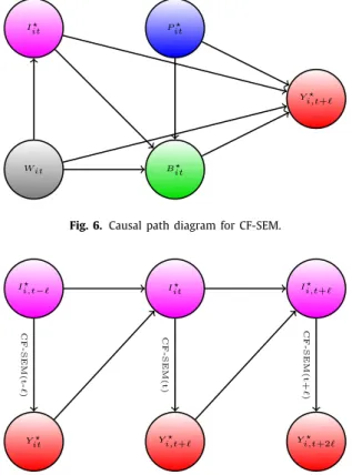
y_itin (SO).

Figs. 6 and7present the causal path diagram for CF-SEM as well as the dynamics of counterfactual information in

CF-SEM.

20 _{This construction is not as efficient as generalized method of moments but has a nicer interpretation under possible misspecification of the}

model: we are combining predictions from two models, one motivated via the causal path, reflecting contextual knowledge, and another from a ‘‘reduced form’’ model not exploiting the path. The combined estimator can improve on precision of either estimator.

21 _{It is possible to consider counterfactual exercises in which policy responds to information through the policy equation if we are interested in}

endogenous policy responses to information. Counterfactual experiments with endogenous government policy would be important, for example, to understand the issues related to the lagged response of government policies to higher infection rates due to incomplete information.

22 _{Furthermore, we conducted several stability checks, for example, checking if the coefficients on mask policies remain stable (reported in the}

(11)

Fig. 6. Causal path diagram for CF-SEM.

Fig. 7. A Diagram for Counterfactual Information Dynamics in CF-SEM.

The counterfactual outcome Y_i⋆_,_t+_ℓand factual outcome Yi,t+_ℓare given by: Y_i⋆_,_t+ℓ

=

(

α

′

β

′

+

π

′)P_it⋆

+

(

α

′

γ

′

+

µ

′)I_it⋆

+

δ

¯

′Wit

+ ¯

ε

yit

,

Yi,t+ℓ

=

(

α

′

β

′

+

π

′)Pit

+

(

α

′

γ

′

+

µ

′)Iit

+

δ

¯

′ Wit

+ ¯

ε

yit

.

In generating these predictions, we explore the assumption of invariance stated above. We can write the counterfactual contrast into the sum of three components:

Y_i⋆_,_t+_ℓ

−

Yi,t+ℓ CF Change

=

α

′

β

′

(

P_it⋆

−

Pit

)

CF Policy Effect via Behavior

+

π

′

(

P_it⋆

−

Pit

)

CF Direct Effect

+

α

′

γ

′

(

I_it⋆

−

Iit

)

+

µ

′

(

I_it⋆

−

Iit

)

CF Dynamic Effect

=:

PEB⋆_it

+

PED⋆_it

+

DynE⋆_it

,

(3)

which describe the immediate indirect effect of the policy via behavior, the direct effect of the policy, and the dynamic effect of the policy. By recursive substitutions the dynamic effect can be further decomposed into a weighted sum of delayed policy effects via behavior and a weighted sum of delayed policy effects via direct impact.

All counterfactual quantities and contrasts can be computed from the expressions given above. For examples, given

∆Ci0

>

0, new confirmed cases are linked to growth rates via relation (taking t divisible by

ℓ

for simplicity):

∆C_it⋆ ∆Ci0

=

exp

(

_t/ℓ

∑

m=1 Y_i⋆_,_m_ℓ

)

and ∆Cit ∆Ci0

=

exp

(

_t/ℓ

∑

m=1 Yi,mℓ

)

.

The cumulative cases can be constructed by summing over the new cases. Various contrasts are then calculated from these quantities. For example, the relative contrast of counterfactual new confirmed cases to the factual confirmed cases

(12)

is given by: ∆C_it⋆ ∆Cit

=

exp

(

_t/ℓ

∑

m=1 (Y_i⋆_,_m_ℓ

−

Yi,mℓ)

)

.

We refer to the appendix for further details. Similar calculations apply for fatalities. Note that our analysis is conditional on the factual history and structural stochastic shocks.23

The estimated counterfactuals are smooth functionals of the underlying parameter estimates. Therefore, we construct the confidence intervals for counterfactual quantities and contrasts by bootstrapping the parameter estimates. We refer to the appendix for further details.

2.4. Outcome and key confounders via SIRD model

We next provide details of our key measurement equations, defining the outcomes and key confounders. We motivate the structural outcome equations via the fundamental epidemiological model for the spread of infectious decease called the Susceptible–Infected–Recovered–Dead (SIRD) model with testing.

Letting Citdenote the cumulative number of confirmed cases in state i at time t, our outcome

Yit

=

∆log(∆Cit)

:=

log(∆Cit)

−

log(∆Ci,t−7) (4)

approximates the weekly growth rate in new cases from t

−

7 to t. Here∆denotes the differencing operator over 7 days from t to t

−

7, so that∆Cit

:=

Cit

−

Ci,t−7is the number of new confirmed cases in the past 7 days.

We chose this metric as this is the key metric for policy makers deciding when to relax Covid mitigation policies. The U.S. government’s guidelines for state reopening recommend that states display a ‘‘downward trajectory of documented cases within a 14-day period’’ (The White House,2020). A negative value of Yit is an indication of meeting this criteria

for reopening. By focusing on weekly cases rather than daily cases, we smooth idiosyncratic daily fluctuations as well as periodic fluctuations associated with days of the week.

Our measurement equation for estimating Eqs.(BPI

→

Y)and(PI

→

Y)will take the form:

∆log(∆Cit)

=

X ′

i,t−14

θ − γ + δ

T∆log(Tit)

+

ϵ

it

,

(M-C)

where i is state, t is day, Cit is cumulative confirmed cases, Tit is the number of tests over 7 days, ∆ is a 7-days

differencing operator, and

ϵ

it is an unobserved error term. Xi,t−14 collects other behavioral, policy, and confounding

variables, depending on whether we estimate(BPI

→

Y)or(PI

→

Y), where the lag of 14 days captures the time lag between infection and confirmed case (seeAppendix A.6). Here

∆log(Tit)

:=

log(Tit)

−

log(Ti,t−7)

is the key confounding variable, derived from considering the SIRD model below. We are treating the change in testing rate as exogenous.24We describe other confounders in the empirical section.

Our main measurement equation(M-C)is motivated by a variant of SIRD model, where we add confirmed cases and infection detection via testing. Let S,I, R, and D denote the number of susceptible, infected, recovered, and deceased individuals in a given state. Each of these variables are a function of time. We model them as evolving as

˙

S(t)

= −

S(t) N

β

(t)I(t) (5)

˙

I(t)

=

S(t) N

β

(t)I(t)

−

γ

I(t) (6)

˙

R(t)

=

(1

−

κ

)

γ

I(t) (7)

˙

D(t)

=

κγ

I(t) (8)

where N is the population,

β

(t) is the rate of infection spread,

γ

is the rate of recovery or death, and

κ

is the probability of death conditional on infection.

Confirmed cases, C (t), evolve as

˙

C (t)

=

τ

(t)I(t)

,

(9)

where

τ

(t) is the rate that infections are detected.

23 _{For unconditional counterfactual, we need to make assumptions about the evolution of stochastic shocks appearing in Y}

it. See, e.g., previous

versions of our paper in ArXiv, where unconditional counterfactuals were calculated by assuming stochastic shocks are i.i.d. and resampling them from the empirical distribution. The differences between conditional and unconditional contrasts were small in our empirical analysis.

24 _{To check sensitivity to this assumption we performed robustness checks, where we used the further lag of}_∆_log(T

it) as a proxy for exogenous

change in the testing rate, and we also used that as an instrument for∆log(Tit); this did not affect the results on policy effects, although the

(13)

Our goal is to examine how the rate of infection

β

(t) varies with observed policies and measures of social distancing behavior. A key challenge is that we only observed C (t) and D(t), but notI(t). The unobservedI(t) can be eliminated by differentiating(9)and using(6)as

¨

C (t)

˙

C (t)

=

S(t) N

β

(t)

−

γ +

˙

τ

(t)

τ

(t)

.

(10)

We consider a discrete-time analogue of Eq.(10)to motivate our empirical specification by relating the detection rate

τ

(t) to the number of tests Titwhile specifying S(t)_N

β

(t) as a linear function of variables Xi,t−14. This results in

∆log(∆Cit) ¨ C (t) ˙ C (t)

=

X_i′_,_t−14

θ + ϵ

it S(t) N β(t)−γ

+

δ

_T∆log(T )it ˙ τ(t) τ(t)

which is equation(M-C), where Xi,t−14captures a vector of variables related to

β

(t).

Structural Interpretation. Early in the pandemic, when the number of susceptibles is approximately the same as the entire population, i.e. Sit

/

Nit

≈

1, the component Xi′,t−14

θ

is the projection of infection rate

β

i(t) on Xi,t−14

(policy, behavioral, information, and confounders other than testing rate), provided the stochastic component

ϵ

itis

orthogonal to Xi,t−14and the testing variables:

β

i(t)Sit

/

Nit

−

γ =

X ′

i,t−14

θ + ϵ

it

, ϵ

it

⊥

Xi,t−14

.

The specification for growth rate in deaths as the outcome is motivated by SIRD as follows. By differentiating(8)and

(9)with respect to t and using(10), we obtain

¨

D(t)

˙

D(t)

=

¨

C (t)

˙

C (t)

−

˙

τ

(t)

τ

(t)

=

S(t) N

β

(t)

−

γ .

(11)

Our measurement equation for the growth rate of deaths is based on Eq.(11)but accounts for a 21 day lag between infection and death as

∆log(∆Dit)

=

X ′

i,t−21

θ + ϵ

it

,

(M-D)

where

∆log(∆Dit)

:=

log(∆Dit)

−

log(∆Di,t−7) (12)

approximates the weekly growth rate in deaths from t

−

7 to t in state i.

3. Empirical analysis

3.1. Data

All code is available athttps://github.com/ubcecon/covid-impact. Our baseline measures for daily Covid-19 cases and deaths are fromThe New York Times (NYT). When there are missing values in NYT, we use reported cases and deaths

fromJHU CSSE, and then theCovid Tracking Project. The number of tests for each state is fromCovid Tracking Project.

As shown in the lower right panel ofFig. A.17in the appendix, there was a rapid increase in testing in the second half of March and then the number of tests increased very slowly in each state in April.

We use the database on US state policies created byRaifman et al.(2020). In our analysis, we focus on 6 policies: stay-at-home, closed nonessential businesses, closed K-12 schools, closed restaurants except takeout, closed movie theaters, and face mask mandates for employees in public facing businesses. We believe that the first four of these policies are the most widespread and important. Closed movie theaters is included because it captures common bans on gatherings of more than a handful of people. We also include mandatory face mask use by employees because its effectiveness on slowing down Covid-19 spread is a controversial policy issue (Howard et al.,2020;Greenhalgh et al.,2020;Zhang et al.,

2020b).Table 1provides summary statistics, where N is the number of states that have ever implemented the policy.

We also obtain information on state-level covariates mostly fromRaifman et al.(2020), which include population size, total area, unemployment rate, poverty rate, a percentage of people who are subject to illness, and state governor’s party affiliations. These confounders are motivated byWheaton and Thompson(2020) who find that case growth is associated with residential density and per capita income.

We obtain social distancing behavior measures from ‘‘Google COVID-19 Community Mobility Reports’’ (Google LLC,

2020). The dataset provides six measures of ‘‘mobility trends’’ that report a percentage change in visits and length of stay at different places relative to a baseline computed by their median values of the same day of the week from January 3 to

(14)

Table 1 State policies.

N Min Median Max

Date closed K 12 schools 51 2020-03–13 2020-03–17 2020-04-03

Stay at home shelter in place 42 2020-03–19 2020-03–28 2020-04-07

Closed movie theaters 49 2020-03–16 2020-03–21 2020-04-06

Closed restaurants except take out 48 2020-03–15 2020-03–17 2020-04-03

Closed non essential businesses 43 2020-03–19 2020-03–25 2020-04-06

Mandate face mask use by employees 44 2020-04–03 2020-05–01 2020-08-03

Fig. 8. The Evolution of Google Mobility Measures: Transit stations and Workplaces. This figure shows the evolution of ‘‘Transit stations’’ and ‘‘Workplaces’’ of Google Mobility Reports. Thin gray lines are the value in each state and date. Thicker colored lines are quantiles of the variables conditional on date. (For interpretation of the references to color in this figure legend, the reader is referred to the web version of this article.)

February 6, 2020. Our analysis focuses on the following four measures: ‘‘Grocery & pharmacy’’, ‘‘Transit stations’’, ‘‘Retail & recreation’’, and ‘‘Workplaces’’.25

Fig. 8shows the evolution of ‘‘Transit stations’’ and ‘‘Workplaces’’, where thin lines are the value in each state and date

while thicker colored lines are quantiles conditional on date. The figures illustrate a sharp decline in people’s movements starting from mid-March as well as differences in their evolutions across states. They also reveal periodic fluctuations associated with days of the week, which motivates our use of weekly measures.

In our empirical analysis, we use weekly measures for cases, deaths, and tests by summing up their daily measures from day t to t

−

6. We focus on weekly cases and deaths because daily new cases and deaths are affected by the timing of reporting and testing and are quite volatile as shown in the upper right panel ofFig. A.17in the appendix. Aggregating to weekly new cases/deaths/tests smooths out idiosyncratic daily noises as well as periodic fluctuations associated with days of the week. We also construct weekly policy and behavior variables by taking 7 day moving averages from day t

−

14 to t

−

21 for case growth, where the delay reflects the time lag between infection and case confirmation. The four weekly behavior variables are referred to ‘‘Transit Intensity’’, ‘‘Workplace Intensity’’, ‘‘Retail Intensity’’, and ‘‘Grocery Intensity’’. Consequently, our empirical analysis uses 7 day moving averages of all variables recorded at daily frequencies. Our sample period is from March 7, 2020 to June 3, 2020.

Table 2reports that weekly policy and behavior variables are highly correlated with each other, except for the‘‘masks

for employees’’ policy. High correlations may cause multicolinearity problems and could limit our ability to separately identify the effect of each policy or behavior variable on case growth. For this reason, we define the ‘‘business closure policies’’ variable by the average of closed movie theaters, closed restaurants, and closed non-essential businesses variables and consider a specification that includes business closure policies in place of these three policy variables separately.

Fig. 9shows the portion of states that have each policy in place at each date. For most policies, there is considerable

variation across states in the time in which the policies are active. The one exception is K-12 school closures. About 80% of states closed schools within a day or two of March 15th, and all states closed schools by early April. This makes the effect of school closings difficult to separate from aggregate time series variation.

3.2. The effect of policies and information on behavior

We first examine how policies and information affect social distancing behaviors by estimating a version of(PI

→

B):

Bj_it

=

(

β

j)′Pit

+

(

γ

j) ′

Iit

+

(

δ

jB) ′

Wit

+

ε

itbj

,

whereBj_itrepresents behavior variable j in state i at time t.Pitcollects the Covid related policies in state i at t. Confounders,

Wit, include state-level covariates, month indicators, and their interactions.Iitis a set of information variables that affect

25 _{The other two measures are ‘‘Residential’’ and ‘‘Parks’’. We drop ‘‘Residential’’ because it is highly correlated with ‘‘Workplaces’’ and ‘‘Retail}

& recreation’’ at correlation coefficients of−0.98 and−0.97, respectively. We also drop ‘‘Parks’’ because it does not have clear implication on the spread of Covid-19.

(15)

Table 2

Correlations among policies and behavior.

workplaces retail grocery transit masks

for employees closed K-12 schools stay at home closed movie theaters closed restaurants closed non-essent bus business closure policies workplaces 1.00 retail 0.93 1.00 grocery 0.75 0.83 1.00 transit 0.89 0.92 0.83 1.00

masks for employees −0.32 −0.17 −0.15 −0.29 1.00

closed K-12 schools −0.91 −0.79 −0.55 −0.72 0.43 1.00

stay at home −0.69 −0.69 −0.70 −0.71 0.28 0.62 1.00

closed movie theaters −0.81 −0.76 −0.64 −0.71 0.34 0.82 0.72 1.00

closed restaurants −0.77 −0.82 −0.68 −0.76 0.21 0.74 0.72 0.82 1.00

closed non-essent bus −0.65 −0.68 −0.68 −0.64 0.08 0.56 0.76 0.68 0.71 1.00

business closure policies −0.84 −0.84 −0.75 −0.79 0.24 0.78 0.81 0.92 0.93 0.87 1.00

Each off-diagonal entry reports a correlation coefficient of a pair of policy and behavior variables. ‘‘business closure policies’’ is defined by the average of closured movie theaters, closured restaurants, and closured non-essential businesses.

Fig. 9. Portion of states with each policy.

people’s behaviors at t. As information, we include each state’s growth of cases (in panel (a)) or deaths (in panel (b)), and log cases or deaths. Additionally, in columns (5)–(8) ofTable 3, we include national growth and log of cases or deaths.

Table 3reports the estimates with standard errors clustered at the state level. Across different specifications, our results

imply that policies have large effects on behavior. Comparing columns (1)–(4) with columns (5)–(8), the magnitude of policy effects are sensitive to whether national cases or deaths are included as information. The coefficient on school closures is particularly sensitive to the inclusion of national information variables. As shown inFig. 9, there is little variation across states in the timing of school closures. Consequently, it is difficult to separate the effect of school closures from a behavioral response to the national trend in cases and deaths.

The other policy coefficients are less sensitive to the inclusion of national case/death variables. After school closures, business closure policies have the next largest effect followed by stay-at-home orders. The effect of masks for employees is small.26

The row ‘‘

∑

jPolicyj’’ reports the sum of the estimated effect of all policies, which is substantial and can account for a

large fraction of the observed declines in behavior variables. For example, inFig. 8, transit intensity for a median state was approximately -50% at its lowest point in early April. The estimated policy coefficients in columns imply that imposing all policies would lead to roughly 75% (in column 4) or roughly 35% (in column 8) of the observed decline. The large impact of policies on transit intensity suggests that the policies may have reduced the Covid-19 infection by reducing people’s use of public transportation.27

26 _{Similar to our finding,}_{Kovacs et al.}₍₂₀₂₀_{) find no evidence that introduction of compulsory face mask policies affect community mobility in}

Germany.