HAL Id: hal-01154264
https://hal.archives-ouvertes.fr/hal-01154264
Submitted on 21 May 2015
HAL is a multi-disciplinary open access
archive for the deposit and dissemination of
sci-entific research documents, whether they are
pub-lished or not. The documents may come from
teaching and research institutions in France or
abroad, or from public or private research centers.
L’archive ouverte pluridisciplinaire HAL, est
destinée au dépôt et à la diffusion de documents
scientifiques de niveau recherche, publiés ou non,
émanant des établissements d’enseignement et de
recherche français ou étrangers, des laboratoires
publics ou privés.
A comparative study of two formal semantics of the
SIGNAL language
Zhibin Yang, Jean-Paul Bodeveix, M Filali
To cite this version:
Zhibin Yang, Jean-Paul Bodeveix, M Filali. A comparative study of two formal semantics of the
SIGNAL language. Frontiers of Computer Science, Springer Verlag, 2013, vol. 7 (n° 5), pp. 673-693.
�10.1007/s11704-013-3908-2�. �hal-01154264�
O
pen
A
rchive
T
OULOUSE
A
rchive
O
uverte (
OATAO
)
OATAO is an open access repository that collects the work of Toulouse researchers and
makes it freely available over the web where possible.
This is an author-deposited version published in :
http://oatao.univ-toulouse.fr/
Eprints ID : 12718
To link to this article :
DOI:10.1007/s11704-013-3908-2
URL :
http://dx.doi.org/10.1007/s11704-013-3908-2
To cite this version :
Yang, Zhibin and Bodeveix, Jean-Paul and Filali,
Mamoun A comparative study of two formal semantics of the SIGNAL
language. (2013) Frontiers of Computer Science, vol. 7 (n° 5). pp. 673-693.
ISSN 2095-2228
Any correspondance concerning this service should be sent to the repository
administrator:
staff-oatao@listes-diff.inp-toulouse.fr
RESEARCH ARTICLE
A comparative study of two formal semantics
of the SIGNAL language
Zhibin YANG 1,2, Jean-Paul BODEVEIX 2, Mamoun FILALI 2 1 School of Computer Science and Engineering, Beihang University, Beijing 100191, China
2 IRIT-CNRS, Université de Toulouse, Toulouse 31062, France
Abstract SIGNAL is a part of the synchronous languages family, which are broadly used in the design of safety-critical real-time systems such as avionics, space systems, and nu-clear power plants. There exist several semantics for SIG-NAL, such as denotational semantics based on traces (called trace semantics), denotational semantics based on tags (called tagged model semantics), operational semantics presented by structural style through an inductive definition of the set of possible transitions, operational semantics defined by syn-chronous transition systems(STS), etc. However, there is lit-tle research about the equivalence between these semantics.
In this work, we would like to prove the equivalence be-tween the trace semantics and the tagged model semantics, to get a determined and precise semantics of the SIGNAL lan-guage. These two semantics have several different definitions respectively, we select appropriate ones and mechanize them in the Coq platform, the Coq expressions of the abstract syn-tax of SIGNAL and the two semantics domains, i.e., the trace model and the tagged model, are also given. The distance between these two semantics discourages a direct proof of e-quivalence. Instead, we transform them to an intermediate model, which mixes the features of both the trace semantics and the tagged model semantics. Finally, we get a determined and precise semantics of SIGNAL.
Keywords synchronous language, SIGNAL, trace seman-tics, tagged model semanseman-tics, semantics equivalence, Coq
E-mail: {Zhibin.Yang, bodeveix, f ilali}@irit. f r
1
Introduction
Safety-critical real-time systems such as avionics, space sys-tems, and nuclear power plants, are also considered as
re-active systems [1], because they always interact with their
environments continuously. The environment can be some physical devices to be controlled, a human operator, or oth-er reactive systems. These systems receive from the envi-ronment input events, and compute the output information, which are finally returned to the environment. The arrival time of events may be different, and the computation need-s time. Synchronouneed-s method ineed-s an important choice to de-sign these systems, which relies on the synchronous
hypothe-sis[2]. Firstly, the computation time is abstracted as zero, that lets system behaviors be divided into a discrete sequence of instants. At each instant, the system does input-computation-output, which takes zero time. Secondly, the different ar-rival time of events are abstracted as the relative order be-tween events. Even of the physical time is abstracted, the inherent functional properties are not changed, so we can say this method focuses on functional behaviors at a platform-independent level.
There are several synchronous languages, such as ESTER-EL [3], LUSTRE [4], SIGNAL [5] and QUARTZ [6]. Syn-chronous languages can be considered as different implemen-tations of the synchronous hypothesis. As a main difference from other synchronous languages, SIGNAL naturally con-siders a mathematical time model, in term of a partial order relation, to describe multi-clocked systems without the
neces-sity of a global clock. This feature permits the description of globally asynchronous locally synchronous systems (GAL-S) [7, 8] conveniently.
There exist several semantics for SIGNAL, such as de-notational semantics based on traces (called trace semantic-s) [9–11], denotational semantics based on tags which are el-ements of a partially ordered dense set (called tagged model semantics) [10,12], operational semantics presented by struc-tural style through an inductive definition of the set of possi-ble transitions [5, 10], operational semantics defined by syn-chronous transition systems (STS) [13]. The differences be-tween the trace semantics and the tagged model semantics are: logical time is represented by a totally ordered set (the set of natural integers N) or a partially ordered set; absence of events is explicitly specified (by the ⊥ symbol) or not. Addi-tionally, Nowak proposes a co-inductive semantics for mod-eling SIGNAL in the Coq proof assistant [14, 15]. However, there is little research about the equivalence between these semantics. The trace semantics and the tagged model seman-tics are more commonly used, so we would like to prove the equivalence between them, to get a determined and precise semantics of the SIGNAL language.
The rest of the paper is organized as follows. Section 2 introduces the basic concepts of the SIGNAL language. The abstract syntax of SIGNAL and its Coq expression is given in Section 3. Section 4 presents the definitions of the two semantics domains, i.e., the trace model and the tagged mod-el. Section 5 gives the two formal semantics and their Coq specifications. The proof of the semantics equivalence is pre-sented in Section 6. Section 7 discusses the related work, and Section 8 gives some concluding remarks.
2
An Introduction to SIGNAL
Signals As declared in the synchronous hypothesis, the be-haviors of a reactive system are divided into a discrete se-quence of instants. At each instant, the system does input-computation-output, which takes zero time. So, the inputs and outputs are sequences of values, each value of the se-quence being present at some instants. Such a sese-quence is called a signal. Consequently, at each instant, a signal may be present or absent (denoted by ⊥). In SIGNAL, signals must be declared before being used, with an identifer (i.e., signal variable or the name of signal) and an associated type for their values such as integer, real, complex, boolean, event, string, etc.
Example 1 Three signals named input1, input2, output
are shown as follows.
input1 1 ⊥ 3 ⊥ · · ·
input2 ⊥ 5 7 9 · · ·
out put ⊥ ⊥10 ⊥ · · ·
Abstract Clock The set of instants where a signal takes a value is the abstract clock of the signal. Two signals are synchronous if they are always present or absent at the same instants, which means they have the same abstract clock.
In the example given above, the abstract clock of input1,
input2and output, denoted respectively ˆinput1, ˆinput2 and
ˆoutput, are defined by different set of logical instants. Moreover, SIGNAL can specify the relations between the abstract clocks of signals in two ways: implicitly or explicit-ly.
Primitive Constructs SIGNAL uses several primitive constructs to express the relations between signals, includ-ing relations between values and relations between abstract clocks. Moreover, the primitive constructs can be classified into two families: monoclock operators (for which all sig-nals involved have the same abstract clock) and multiclock operators (for which the signals involved may have different clocks).
• Monoclock operators, including instantaneous
func-tion and delay. The instantaneous function x :=
f(x1,· · · , xn) applied on a set of inputs x1,· · · , xn will
produce the output x, while the delay operator x :=
x1 $ init c sends a previous value of the input to the
output with an initial value c.
• Multiclock operators, including undersampling and
de-terministic merging. The undersampling operator x :=
x1when x2is used to check the output of an input at the
true occurrence of another input, while the deterministic merging operator x := x1de f ault x2is used to select
be-tween two inputs to be sent as the output, with a higher priority to the first input.
Notice that, these operators specify the relations between the abstract clocks of the signals in an implicit way.
In the SIGNAL language, the relations between values and the relations between abstract clocks, of the signals, are de-fined as equations, and a process consists of a set of equation-s. Two basic operators apply to processes, the first one is the
compositionof different processes, and the other one is the
local declarationin which the scope of a signal is restricted
to a process.
Example 2 Let us consider a simple process Count [12]. It accepts an input signal reset and delivers the integer output
signal val. The local variable counter is initialized to 0 and s-tores the previous value of the signal val. When an input reset occurs, the signal val is reset to 0. Otherwise, the signal val takes an increment of the variable counter. The process
Par-allelCountis the composition of two Count processes. Here,
the program is not deterministic.
process ParallelCount = (! integer x1, x2; )
(| x1 := Count(r) | x2 := Count(r) |) where event r;
process Count = (? event reset; ! integer val; )
(| counter := val $1 init 0
| val := (0 when reset) de f ault (counter + 1) |) where integer counter;
end;
end;
Extended Constructs SIGNAL also provides some oper-ators to express control-related properties by specifying clock relations explicitly, such as clock synchronization, set op-erators on clocks (union, intersection, difference) and clock comparison.
• Clock synchronization, the equation x1ˆ= x2ˆ= · · · ˆ=xn
specifies that signals x1,x2,· · · , xnare synchronous.
• Set operators on clocks, such as the equation x:= x1ˆ +
x2 defines the clock of x as the union of the clocks of
signals x1and x2, the equation x:= x1ˆ * x2defines the
clock of x as the intersection of the clocks of signals x1
and x2, the equation x:= x1ˆ - x2defines the clock of x
as the difference of the clocks of signals x1and x2.
• Clock comparison, such as the statement x1ˆ < x2
speci-fies a set inclusion relation between the clocks of signals
x1and x2, the statement x1ˆ > x2specifies a set
contain-ment relation between the clocks of signals x1and x2.
3
Abstract Syntax of SIGNAL and its Coq
Ex-pression
In this section, we first give a brief introduction of the theo-rem prover Coq, then, we give the abstract syntax of SIGNAL and its Coq expression.
3.1 A Brief Introduction of Coq
Coq [16] is a theorem prover based on the Calculus of Induc-tive Constructions which is a variant of type theory, follow-ing the "Curry-Howard Isomorphism" paradigm, enriched with support for inductive and co-inductive definitions of data
types and predicates. From the specification perspective, Co-q offers a rich specification language to define problems and state theorems. From the proof perspective, proofs are devel-oped interactively using tactics, which can reduce the work-load of the users. Moreover, the type-checking performed by Coq is the key point of proof verification.
Here, we try to give an intuitive introduction to the Co-q terminologies which are used in this paper. In the spirit of "Curry-Howard Isomorphism" paradigm, types may rep-resent programming data-types or logical propositions. So, the Coq objects used in this paper can be sorted into two cat-egories: the Type sort and the Prop sort:
• Typeis the sort for data types and mathematical struc-tures, i.e. well-formed types or structures are of type
Type. Data types can be basic types such as nat,
bool, nat → nat, etc., and can be inductive structures,
recordand co-inductive structures (for infinite objects,
as for example infinite sequences). We use Fixpoint and
CoFixpointdefinitions to define functions over inductive
and to co-inductive data types.
• Propis the sort for propositions, i.e. well-formed propo-sitions are of type Prop. We can define new predicates using inductive, record (for conjunctions of properties) or co-inductive definitions.
3.2 The Abstract Syntax of SIGNAL
The semantics of each of the extended constructs is defined in term of the primitive constructs, so we just consider the primitive constructs, that is core-SIGNAL. Its abstract syntax is presented as follows.
P::= x := f (x1,· · · , xn) instantaneous f unction
|x:= x1$ init c delay
|x:= x1when x2 undersampling
|x:= x1de f ault x2deterministic merging
|P|P′ composition
|P/x local declaration
To express more complex SIGNAL programs, all the right-side signal variables of the equations can be replaced by an expression on signal variables.
Here we give the Coq expression of the abstract syntax of SIGNAL. It is parameterized by the set XVar of signal variables, and the set Value of values that can be taken by the variables. isTrue checks that a value is considered to be true. mkBool is used to coerce Bool(s) to Value(s). The type
Processis defined using five constructors corresponding to
the constructs of the core-SIGNAL. We give a very abstract expression of an instantaneous function. The function Pass
takes three parameters: a function f of type ((Index →
Val-ue) → ValVal-ue)having an indexed set of input parameters, a
variable name of type XVar which contains the left-side vari-able and an indexed set of varivari-able names of type (Index →
XVar)which denotes the actual parameters of f . Index, for
example 1, · · · , n, represents a set used to index the parame-ters. Similarly, Pdelay, Pwhen, Pdefault, and Ppar build the corresponding SIGNAL constructs. However, the local dec-laration is ignored, to get a simplest criterion for the proof of semantics equivalence (see Section 5 and Section 6).
Parameter XVar : Type . Parameter V a l u e : Type .
Parameter i s T r u e : V a l u e → Prop . Parameter mkBool : Bool → V a l u e . I n d u c t i v e P r o c e s s : Type : =
P a s s : ∀ I n d e x , ( ( I n d e x → V a l u e ) → V a l u e ) → XVar → ( I n d e x → XVar ) → P r o c e s s | P d e f a u l t : XVar → XVar → XVar → P r o c e s s | Pwhen : XVar → XVar → XVar → P r o c e s s | P d e l a y : XVar → XVar → V a l u e → P r o c e s s | P p a r : P r o c e s s → P r o c e s s → P r o c e s s .
4
Semantics Domains
Semantics domains such as the trace model and the tagged model are introduced in this section. To avoid confusion, we will treat signal variables and signals (sequence of values) separately. The naming convention is given as follows:
• { x, x1, x2, . . . , xn, y, . . . } are signal variables.
• { v, v1, v2, . . . , vn, vv, c, . . . } are values, and c represents
a constant value.
• { s, s1, s2, . . . , sn, . . . } are signals.
• { i, i1, i2, . . . , in, j, k, . . . } are indexes.
• { tr, tr1, tr2, . . . , trn, tr′, trs, . . . } are traces.
• { t, t0, t1, . . . , tn, tt, . . . } are tags.
• { b, b1, b2, . . . , bn, b′, tb, . . . } are the behaviors on tag
structures.
The SIGNAL language specifies a system behavior as a platform-independent model at first. However, it is finally needed to guarantee a correct physical implementation from it (i.e., need to deal with physical time). A formal support for allowing time scalability in design is given in the modeling environment Polychrony [17] by the so-called stretch-closure property. This property can be defined both on the trace mod-el and on the tagged modmod-el.
4.1 Trace Model
Let X be a set of signal variables, and let V be the set of values that can be taken by the variables. The symbol ⊥ (⊥ <V) is introduced to express the absence of valuation of a variable. Then we denote:
V⊥ =V ∪ {⊥}
The corresponding Coq expression is given as follows: I n d u c t i v e EValue : Type : =
Val : V a l u e → EValue | A bs en c e : EValue .
Definition 1 (VSignal) [10] A signal s is a sequence (si)i∈I of typed values (of V⊥), where I is the set of natural
integers N or an initial segment of N, including the empty segment.
A signal can be finite. However, we can extend the finite signal with infinite absences, to get an infinite one. So, in the Coq expression, a signal is defined as an infinite object.
C o I n d u c t i v e V S i g n a l : Type : =
Vs : EValue → V S i g n a l → V S i g n a l .
In the following paragraphs, the definition of traces is giv-en. Notice that, a signal is just a sequence of values corre-sponding to a signal variable, while a trace defines the syn-chronized sequences of values of a set of signal variables.
Definition 2 (Event) [9] Considering X a non-empty sub-set of X, we call event on X any application
e: X → V⊥X
• e(x) = ⊥ indicates that variable x has no value in the event.
• e(x) = v indicates, for v ∈ Vx, that variable x takes the
value v in the event.
The absent event on X (X → {⊥}), where all the signals are absent at a logical instant, is denoted ⊥e(X). Moreover, the
set of events on X (X → V⊥
X) is denoted
ε
X.A trace is a sequence of events. For any subset X of X, we consider the following definition of the set
τ
X of traces onX.
Definition 3 (Traces)
τ
X is the set of traces on X,de-fined as the set of applications N →
ε
X where N is the set ofnatural integers.
The absent trace on X (N → {⊥e(X)}), i.e., the infinite
se-quence formed by the infinite repetition of ⊥e(X), is denoted
⊥X.
Similarly, a trace can be finite. However, we can extend the finite sequence with infinite absent events, to get an infi-nite trace.
Example 3 Let us consider the following equation: x3:=
x1∗ x2. The set of signal variables is X = {x1, x2, x3}. A
possible trace is given as follow:
x1⊥ 3 3 ⊥ ⊥ 0 · · ·
x2⊥ 5 7 ⊥ ⊥ 9 · · ·
x3⊥15 21 ⊥ ⊥ 0 · · ·
The trace can be seen as a sequence of events:
{e0: x17→ ⊥ x27→ ⊥ x37→ ⊥ ,e1: x17→3 x27→5 x37→15 ,· · · }
The Coq expression of the definition of traces is given as follows.
C o I n d u c t i v e T r a c e : Type : =
Tr : ( XVar → EValue ) → T r a c e → T r a c e . As mentioned before, the set of instants where a signal takes a value is the abstract clock of the signal. Its Coq ex-pression is given as follows.
C o F i x p o i n t AClock ( x : XVar ) ( t r : T r a c e ) : V S i g n a l : = match t r w i t h Tr s t t r ’ ⇒ match s t x w i t h A bs e nc e ⇒ Vs A bs en c e ( AClock x t r ’ ) |_ ⇒ Vs ( Val ( mkBool t r u e ) ) ( AClock x t r ’ ) end end.
Definition 4 (Sprocess) Given a SIGNAL process, its trace semantics, denoted as Sprocess, includes a set of sig-nal variables defining the domain of the process and a set of traces.
The Coq expression is given as follows: Record S p r o c e s s : Type : = {
sdom : XVar → Prop ; s t r a c e s : T r a c e → Prop } .
Additionally, we give the definition of the stretch-closure property on the trace model as the definition of compression of a trace given in [18]. The intuition is to consider a trace as an elastic with ordered marks on it. If it is stretched, the marks remain in the same order but have more space (time) between each other by adding columns of ⊥ (see Fig.1). The same holds for a set of traces (a behavior), so stretching gives rise to an equivalence between behaviors (stretch equiv-alence).
Definition 5 (Stretching) For a given subset X of X, a trace tr1is less stretched than another trace tr2, noted tr1≤τX tr2, iff there exists a mapping f : N → N such as:
Fig. 1 Stretching of a trace following f
• ∀x ∈ X ∀i ∈ N, tr2( f (i))(x) = tr1(i)(x)
• ∀x ∈ X ∀ j ∈ N, tr2( j)(x) = ⊥, i f j < range( f )
• ∀i j ∈ N, i < j ⇒ f(i) < f ( j)
The Coq expression is given as follows. trGetEV is used to get the value (including ⊥) of each signal at each instant of a trace. F i x p o i n t t r G e t E V t r i x : EValue : = match i , t r w i t h O, ( Tr s t t r ’ ) ⇒ s t x | ( S j ) , ( Tr s t t r ’ ) ⇒ t r G e t E V t r ’ j x end. Record S t r e t c h i n g ( t r 1 : T r a c e ) ( t r 2 : T r a c e ) : Prop : = { S t r e t c h _ f : n a t → n a t ; S t r e t c h _ v a l : ∀ x i , t r G e t E V t r 1 i x = t r G e t E V t r 2 ( S t r e t c h _ f i ) x ; S t r e t c h _ b o t : ∀ x j , ( ∀ i , S t r e t c h _ f j , i ) → t r G e t E V t r 2 j x = A bs en c e ; S t r e t c h _ m o n o : ∀ i j , i < j → S t r e t c h _ f i < S t r e t c h _ f j } .
Definition 6 (Stretch Equivalence) For a given subset
X of X, two traces tr1 and tr2 are stretch-equivalent, noted
tr1 ≷ tr2, iff there exists another behavior tr3 less stretched
than both tr1and tr2, i.e., tr1 ≷ tr2 iff ∃tr3tr3 ≤τX tr1 and tr3≤τX tr2.
The Coq expression is given as follows:
I n d u c t i v e S t r e t c h _ E q u i v a l e n c e ( t r 1 : T r a c e ) ( t r 2 : T r a c e ) : Prop : =
S t r _ E q P r f : ∀ t r 3 : T r a c e , S t r e t c h i n g t r 3 t r 1 → S t r e t c h i n g t r 3 t r 2
→ S t r e t c h _ E q u i v a l e n c e t r 1 t r 2 . Definition 7 (Stretch Closure) For a given trace tr, the set of all traces that are stretch-equivalent to tr, defines its
stretch closure, noted tr*.
The stretch closure of a set of traces
τ
X, includes all thetraces resulting from the stretch closure of each trace tr ∈ τX,
i.e.,S
tr∈τXtr
The Coq expression is given as follows: I n d u c t i v e S t r e t c h _ C l o s u r e ( t r s : T r a c e → Prop ) : T r a c e → Prop : = S t r e t c h _ c l : ∀ t r 1 t r 2 : T r a c e , t r s t r 1 → S t r e t c h _ E q u i v a l e n c e t r 1 t r 2 → S t r e t c h _ C l o s u r e t r s t r 2 . Definition 8 (Stretch-Closed) A SIGNAL process is stretch-closed, iff, for all tr′ ∈ S process.stracesand for all
tr ∈ τX, tr ≷ tr′⇒ tr ∈ S process.straces
4.2 Tagged Model
Lee and Sangiovanni-Vincentelli proposed the tagged-signal model [19] to compare various models of computation. It is a denotational approach where a system is modeled as a set of behaviors. Behaviors are sets of events. Each event is a value-tag pair. Complex systems are derived through the parallel composition of sub-systems, by taking the intersection of the sets of behaviors. After that, the tagged-signal model is also used to express the semantics of the SIGNAL language [10, 12], because this model can represent the feature of multi-clock naturally.
We reuse the sets X and V defined in Section 4.1.
Definition 9 (Tag Structure) A tag structure is a tuple (T, ≤), where:
• Tis the set of tags. • ≤is a partial order on T.
The Coq expression is given as follows. Tag represents a set of tags, tle is a partial order, and tlt is defined as a strict partial order.
Record TAG : Type : = { Tag : Type ;
t l e : Tag → Tag → Prop ; t p o : o r d e r Tag t l e ;
t l t t 1 t 2 : = t l e t 1 t 2 ∧ t 1 , t 2 ; } .
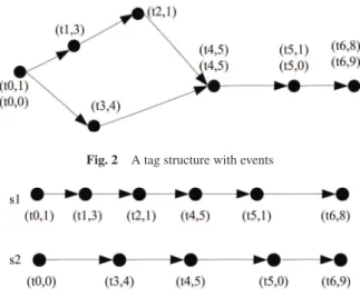
Definition 10 (Tagged Event) [10] A tagged event e on a given tag structure (T, ≤) is a pair (t, v) ∈ T × V.
Example 4 A tag structure associated with events is given in Fig.2. Sharing the same tag among different events repre-sents the events are synchronous at that logical instant.
A totally ordered set of tags C ∈ T is called a chain, and
min{C}denotes the minimum element of C. In addition, we
denote by CTthe set of all chains on (T, ≤).
Definition 11 (TSignal) A signal on a tag structure (T, ≤) is a partial function s ∈ C ⇀ V which associates values with the tags that belong to a chain C.
Let the set of signals on (T, ≤) be noted ST. Here, we give
two signals as an example (see Fig.3).
Fig. 2 A tag structure with events
Fig. 3 Two signals of the tag structure in Fig.2
The Coq expression is given as follows. The type
Tsig-nal_fromis used to construct a chain from a tag t. Tsignal
represents the set of signals. "@<" is the notation for the strict partial order tlt.
C o I n d u c t i v e T s i g n a l _ f r o m {G : TAG} ( t : Tag G ) : Type : = Tend : T s i g n a l _ f r o m t | T n e x t : ∀ t n , t @< t n → V a l u e → T s i g n a l _ f r o m t n → T s i g n a l _ f r o m t . I n d u c t i v e T s i g n a l G : Type : = Tempty : T s i g n a l G | Tfrom : ∀ ( t : Tag G) , V a l u e → T s i g n a l _ f r o m t → T s i g n a l G .
Definition 12 (Behavior) Given a tag structure (T, ≤), a behavior b on X ⊆ X is a function b ∈ X → STthat associates
each variable x ∈ X with a signal s on (T, ≤).
Notice that, here signal variables and signals are treated separately, and the behaviors on tag structures give the map-ping between them.
The Coq expression is given as follows. In the type
Tbe-havior, each variable is associated with a signal.
D e f i n i t i o n T b e h a v i o r (G : TAG) : = XVar → T s i g n a l G .
We denote by B|X the set of behaviors of domain X ⊆ X
on (T, ≤). Given a behavior b ∈ B|X, we write vars(b) and
tags(b(x))(x ∈ vars(b)) to denote the signal variables
consid-ered in b and the set of tags associated with the signal variable
x. 0|Xexpresses the association of X with empty signal.
Definition 13 (Tprocess) Given a SIGNAL process, its tagged model semantics, denoted as Tprocess, includes a set of signal variables and a set of behaviors on tag structures.
The Coq expression is given as follows: Record T p r o c e s s (G : TAG) : = {
t b e h a v i o r s : T b e h a v i o r G → Prop } .
Remark 1 The logical time used in the trace model is a totally ordered set, and the absence of events is explicitly specified, while the logical time used in the tagged model is a partially ordered set, and the absence of events is not specified. Moreover, a tag structure may correspond to a set of traces.
Additionally, we give the definition of the stretch-closure property on the tagged model [10, 12]. The intuition is to consider a signal as an elastic with tags on it. If it is stretched, tags remain in the same order but have more space (time) between each other (see Fig.4). The same holds for a set of elastics: a behavior. If elastics are equally stretched, the partial order between tags is unchanged.
Fig. 4 Stretching of a behavior composed of two signals following f
Definition 14 (Stretching) For a given domain X ⊆ X, a behavior b1is less stretched than another behavior b2, noted
b1≤B|X b2, iff there exists a mapping f : tags(b1) → tags(b2)
following b1and b2are isomorphic:
• ∀x ∈ vars(b1), f (tags(b1(x))) = tags(b2(x))
• ∀x ∈ vars(b1) ∀t ∈ tags(b1(x)), b1(x)(t) = b2(x)( f (t))
• ∀t1,t2∈ tags(b1), t1<t2 ⇒ f(t1) < f (t2)
• ∀C ∈ CT,∀t ∈ C, t ≤ f(t)
The Coq expression is given as follows. tags_ f rom and
tagsare used to get the tags of a given signal, btags repre-sents the tags of all the signals in a given behavior, while
tval_ f rom and tval are used to get the value at each tag of a signal. "@<=" is the notation of tle.
I n d u c t i v e t a g s _ f r o m {G} ( t t 0 : Tag G) : T s i g n a l _ f r o m t 0 → Prop : = i n _ c u r r : ∀ t i h v i s ’ , t = t i → t a g s _ f r o m t t 0 ( T n e x t t 0 t i h v i s ’ ) | i n _ n e x t : ∀ t i h v i s ’ , t a g s _ f r o m t t i s ’ → t a g s _ f r o m t t 0 ( T n e x t t 0 t i h v i s ’ ) . I n d u c t i v e t a g s {G} t : T s i g n a l G → Prop : = i n _ f i r s t : ∀ t 0 v0 s ’ , t 0 = t → t a g s t ( Tfrom G t 0 v0 s ’ ) | i n _ f r o m : ∀ t 0 v0 s ’ , t a g s _ f r o m t t 0 s ’ → t a g s t ( Tfrom G t 0 v0 s ’ ) . I n d u c t i v e b t a g s {G} ( b : T b e h a v i o r G) ( dom : XVar → Prop ) t : Prop : =
b t a g s P r f : ∀ x , dom x → t a g s t ( b x ) → b t a g s b dom t .
Record t S t r e t c h i n g {G1 G2 : TAG} ( b1 : T b e h a v i o r G1 ) ( b2 : T b e h a v i o r G2 ) ( dom : XVar → Prop ) : Prop : = {
t S t r e t c h _ f : Tag G1 → Tag G2 ; t S t r e t c h _ t a g s : ∀ t 2 x , dom x → t a g s t 2 ( b2 x ) → ∃ t 1 , t a g s t 1 ( b1 x ) ∧ t 2 = t S t r e t c h _ f t 1 ; t S t r e t c h _ v a l : ∀ t x v , dom x → t v a l ( b1 x ) t v → t v a l ( b2 x ) ( t S t r e t c h _ f t ) v ; t S t r e t c h _ m o n o : ∀ t 1 t 2 : Tag G1 , b t a g s b1 dom t 1 → b t a g s b1 dom t 2 → t 1 @< t 2 → t S t r e t c h _ f t 1 @< t S t r e t c h _ f t 2 ; t S t r e t c h _ i n c r : ∀ t , t @<= t S t r e t c h _ f t } .
Definition 15 (Stretch Equivalence) For a given domain
X ⊆ X, two behaviors b1and b2are stretch-equivalent, noted
b1≷b2, iff there exists another behavior b3less stretched than
both b1and b2, i.e., b1≷b2iff ∃b3b3≤B|X b1and b3≤B|X b2.
The Coq expression is given as follows.
I n d u c t i v e t S t r e t c h _ E q u i v a l e n c e {G1 G2 : TAG} ( b1 : T b e h a v i o r G1 ) ( b2 : T b e h a v i o r G2 )
( dom : XVar → Prop ) : Prop : =
t S t r E q : ∀ G3 ( b3 : T b e h a v i o r G3 ) , t S t r e t c h i n g b3 b1 dom → t S t r e t c h i n g b3 b2 dom
→ t S t r e t c h _ E q u i v a l e n c e b1 b2 dom . Definition 16 (Stretch Closure) For a given behavior b, the set of all behaviors that are stretch-equivalent to b, defines its stretch closure, noted b*.
The stretch closure of a set of behaviors B|Xincludes all the
behaviors resulting from the stretch closure of each behavior
b ∈ B|X, i.e.,Sb∈B|Xb ∗.
The Coq expression is given as follows. I n d u c t i v e t S t r e t c h _ C l o s u r e {G : TAG}
( t b : T b e h a v i o r G → Prop ) ( dom : XVar → Prop) : T b e h a v i o r G → Prop : =
t S t r e t c h _ c l : ∀ b1 b2 , t b b1
→ t S t r e t c h _ E q u i v a l e n c e b1 b2 dom → t S t r e t c h _ C l o s u r e t b dom b2 .
Definition 17 (Stretch-Closed) A SIGNAL process is stretch-closed, iff, for all b′ ∈ T process.tbehaviorsand for
all b ∈ B|X, b ≷ b′⇒ b ∈ T process.tbehaviors
5
Two Formal Semantics
Primitive constructs of the SIGNAL language specify the re-lations between signals at the syntax level. The trace seman-tics and the tagged model semanseman-tics are both denotational style. They interpret and define precisely the relations be-tween values and the relations bebe-tween clocks of signals in their semantics domains. In this paper, the semantics ignores the local declaration of signal variables to get a simplest cri-terion for the proof of semantics equivalence.
5.1 Trace Semantics
There are several definitions of the trace semantics of SIG-NAL [9–11], we select [10] as the reference paper semantics and mechanize it in Coq. Most of the Coq expressions are close to the paper semantics, but some expressions are not, so we need to justify the equivalence between them. We also refer to the Coq expressions of Nowak [14, 15].
Here, each single signal is observed in the reference pa-per semantics, while the corresponding trace with signal vari-ables x, x1, . . . ,xn is directly used in the Coq expressions.
The difference between them has been given in Section 4.1. The mapping between them is done at the end (i.e., the defi-nition Process2Sprocess).
Trace Semantics 1 (Instantaneous function) The trace semantics of the instantaneous function is defined as follows:
∀τ ∈N
sτ=
( ⊥ i f s1τ = . . . =snτ=⊥
f(s1τ, . . . ,snτ) i f s1τ ,⊥ ∧ . . . ∧ snτ,⊥
At each instant τ, the signals are either all present or all absent, i.e., they are synchronous, denoted as s ˆ = s1ˆ = · · · ˆ
= sn. sτgets the value of f (s1τ, . . . ,snτ) when the signals are
all present. The function f includes different mathematical operations, such as arithmetic operations, boolean operations, etc.
The corresponding Coq expression is given as follows. C o I n d u c t i v e S a s s i g n m e n t x I n d e x ( f : ( I n d e x → V a l u e ) → V a l u e ) ( x i : I n d e x → Var ) : T r a c e → Prop : = SassU : ∀ s t t r , ( ∀ i , s t ( x i i ) = A bs e nc e ) → s t x = A bs e nc e → S a s s i g n m e n t x I n d e x f x i t r → S a s s i g n m e n t x I n d e x f x i ( Tr s t t r ) | S a s s P : ∀ v s t t r , ( ∀ i , s t ( x i i ) = Val ( v i ) ) → s t x=Val ( f v ) → S a s s i g n m e n t x I n d e x f x i t r → S a s s i g n m e n t x I n d e x f x i ( Tr s t t r ) . Trace Semantics 2 (Delay)The trace semantics of the de-lay construct is defined as follows:
−(∀τ ∈ N) s1τ=⊥ ⇔ sτ=⊥
− {k | s1k,⊥} , ∅ ⇒ smin{k|s1k,⊥}=c
−(∀τ ∈ N) s1τ,⊥ ∧ {k > τ | s1k,⊥} , ∅
⇒ smin{k>τ|s1k,⊥}=s1τ
Here, we make the definition of the trace semantics of
De-lay in [10] more precise. min(S) denotes the minimum of a non-empty set of naturals. Similarly to the instantaneous function, the delay construct also requires signals s and s1
have the same clock, denoted as s ˆ= s1. Given a logical
in-stant τ, s takes the most recent value of s1except the one at
τ. Initially, s takes the value c.
The Coq expression is given as follows.
C o I n d u c t i v e S d e l a y x x1 c : T r a c e → Prop : = S de la yU : ∀ s t t r , s t x1 = A bs e nc e → s t x = A bs e nc e → S d e l a y x x1 c t r → S d e l a y x x1 c ( Tr s t t r ) | S d e l a y P : ∀ s t v t r , s t x1 = Val v → s t x = Val c → S d e l a y x x1 v t r → S d e l a y x x1 c ( Tr s t t r ) .
Trace Semantics 3 (Undersampling)The trace semantics of the undersampling construct is defined as follows:
∀τ ∈N
sτ=
( s1τi f s2τ=true
⊥ otherwise
Here, s and s1have the same type and s2is a boolean
sig-nal. The clock of s is the intersection of the clock of s1 and
the clock of s2, denoted as s=s1ˆ * [s2], while [s2] represents
the true occurrences of s2. Given a logical instant τ, sτgets
the value of s1τwhen s2τis true, else gets the value ⊥.
The Coq expression is given as follows.
C o I n d u c t i v e Swhen ( x x1 x2 : XVar ) : T r a c e→Prop : = SwhenT : ∀ s t v b t r , i s T r u e b → s t x = Val v → s t x1 = Val v → s t x2 = Val b → Swhen x x1 x2 t r → Swhen x x1 x2 ( Tr s t t r ) | SwhenF : ∀ s t b t r , ¬ i s T r u e b → s t x = A bs e nc e → s t x2 = Val b → Swhen x x1 x2 t r → Swhen x x1 x2 ( Tr s t t r ) | SwhenU : ∀ s t t r , s t x = A bs e nc e → s t x2 = A bs e nc e → Swhen x x1 x2 t r → Swhen x x1 x2 ( Tr s t t r ) .
Trace Semantics 4 (Deterministic merging) The trace semantics of the deterministic merging construct is defined as follows:
∀τ ∈N
sτ=
( s1τi f s1τ,⊥
s2τotherwise
Here, signals s, s1and s2have the same type. The clock of
sis the union of the clocks of s1and s2, denoted as s = s1ˆ +
s2. Given a logical instant τ, sτgets the merge of the values
of s1τand s2τ, and the value of s1τhas a higher priority.
The Coq expression is given as follows.
C o I n d u c t i v e S d e f a u l t ( x x1 x2 : Var ) : T r a c e→Prop : = S d e f a u l t U : ∀ s t t r , s t x = A bs e nc e → s t x1 = A bs en c e → s t x2 = A bs en c e → S d e f a u l t x x1 x2 t r → S d e f a u l t x x1 x2 ( Tr s t t r ) | S d e f a u l t 1 : ∀ s t v t r , s t x = Val v → s t x1 = Val v → S d e f a u l t x x1 x2 t r → S d e f a u l t x x1 x2 ( Tr s t t r ) | S d e f a u l t 2 : ∀ s t v t r , s t x = Val v → s t x1 = A bs en c e → s t x2 = Val v → S d e f a u l t x x1 x2 t r → S d e f a u l t x x1 x2 ( Tr s t t r ) . Finally, we apply these semantics rules to a SIGNAL process, to get a complete semantics of the process, that is Sprocess (defined in Section 4.1). SPassignment,
SPde-lay, SPwhen and SPdefault, used to construct the corre-sponding Sprocess on the semantics rule Sassignment,
Sde-lay, Swhen and Sdefault respectively, while the function
Pro-cess2Sprocessis used to combine them as one Sprocess. We
also give the semantics of processes composition, that is
SP-prod. P ro gr am D e f i n i t i o n S P a s s i g n m e n t x I n d f x i : = { | sdom y : = y=x ∨ ∃ i , y= x i i ; s t r a c e s t r : = S a s s i g n m e n t x I n d f x i t r |} . P ro gr am D e f i n i t i o n S P d e l a y x x1 c : = { |
sdom y : = y=x ∨ y=x1 ;
s t r a c e s t r : = S d e l a y x x1 c t r |} .
P ro gr am D e f i n i t i o n SPwhen x x1 x2 : = { |
sdom y : = y=x ∨ y=x1 ∨ y=x2 ; s t r a c e s t r : = Swhen x x1 x2 t r |} .
P ro gr am D e f i n i t i o n S P d e f a u l t x x1 x2 : = { |
sdom y : = y=x ∨ y=x1 ∨ y=x2 ; s t r a c e s t r : = S d e f a u l t x x1 x2 t r
|} .
Pr og ra m D e f i n i t i o n SPprod p1 p2 : = { |
sdom y : = sdom p1 y ∨ sdom p2 y ; s t r a c e s t r : = s t r a c e s p1 t r ∧ s t r a c e s p2 t r |} . F i x p o i n t P r o c e s s 2 S p r o c e s s ( p : P r o c e s s ) : S p r o c e s s : = match p w i t h P a s s I n d f x x i ⇒ S P a s s i g n m e n t x I n d f x i | Pwhen x x1 x2 ⇒ SPwhen x x1 x2 | P d e l a y x x1 c ⇒ S P d e l a y x x1 c | P d e f a u l t x x1 x2 ⇒ S P d e f a u l t x x1 x2 | P p a r p1 p2 ⇒ SPprod ( P r o c e s s 2 S p r o c e s s p1 ) ( P r o c e s s 2 S p r o c e s s p2 ) end.
Example 5 The trace semantics of the process
Parallel-Count(example 2) is a set of traces, and two possible traces
are given as follows. Here, we just consider the external visi-ble signals (the local declarations are hidden).
tr1 : x1 1 ⊥ 2 ⊥ 0 1 ⊥ 2 ⊥ 3 ⊥ 0 ⊥ . . .
x2 ⊥ 1 ⊥ 2 0 ⊥ 1 ⊥ 2 ⊥ 3 0 ⊥ . . .
tr2 : x1 0 1 2 ⊥ 0 1 2 ⊥ 3 0 ⊥ . . .
x2 0 ⊥ ⊥ 1 0 ⊥ ⊥ 1 ⊥ 0 ⊥ . . .
Property 1 For all SIGNAL processes, the trace seman-tics is stretch-closed.
5.2 Tagged Model Semantics
Similarly, there are several definitions of the tagged model semantics of SIGNAL [10,12], we select [10] as the reference paper semantics and mechanize it in Coq.
Here, signal variables x, x1, . . . ,xn are used in the
refer-ence paper semantics, while the tag structure with signals
s, s1, . . . ,snis used in the Coq expressions. The relation
be-tween them has been shown in Section 4.2. The mapping between them is done at the end (i.e., the definition
Pro-cess2Tprocess).
Tagged Model Semantics 1 (Instantaneous function) The tagged model semantics of the instantaneous function is defined as follows:
Jx := f (x1,· · · , xn)K =
{b ∈ B|x,x1,··· ,xn|tags(b(x)) = tags(b(x1)) = · · · = tags(b(xn))
=C ∈ CT and ∀t ∈ C, b(x)(t) =J f K(b(x1)(t), · · · , b(xn)(t))}
The semantics of the instantaneous function is the set of behaviors b. The tags of each signal involved in b represent the same chain C, i.e., all the signals are synchronous. When
the signals are all present, at each tag of C, the output signal gets the corresponding value.
The corresponding Coq expression is given as follows.
T-SA_T is used to express the relation between values, while
TSA_Srepresents all the signals are synchronous. tval_from
and tval represent that, given a signal of a tag structure G and a tag of the signal, we can get the corresponding value. tsync means two signals are synchronous.
I n d u c t i v e t v a l _ f r o m {G} ( t 0 : Tag G ) : T s i g n a l _ f r o m t 0 → Tag G → V a l u e → Prop : = t v _ c u r r : ∀ t h v s t t vv , t = t t → v=vv → t v a l _ f r o m t 0 ( T n e x t t 0 t h v s ) t t vv | t v _ n e x t : ∀ t h v s t t vv , t v a l _ f r o m t s t t vv → t v a l _ f r o m t 0 ( T n e x t t 0 t h v s ) t t vv . I n d u c t i v e t v a l {G} : T s i g n a l G → Tag G → V a l u e → Prop : = t v _ f i r s t : ∀ t v s t t vv , t = t t → v=vv → t v a l ( Tfrom G t v s ) t t vv | t v _ f r o m : ∀ t 0 v s t t vv , t v a l _ f r o m t 0 s t t vv → t v a l ( Tfrom G t 0 v s ) t t vv . D e f i n i t i o n t s y n c {G} ( s 1 s 2 : T s i g n a l G ) : Prop : = ∀ t , t a g s t s 1 ↔ t a g s t s 2 . Record T S a s s i g n m e n t {G} s I n d e x ( f : ( I n d e x → V a l u e ) → V a l u e ) ( s i : I n d e x → T s i g n a l G) : Prop : = { TSA_T : ∀ t d v , ( ∀ i , t v a l ( s i i ) t ( d i ) ) → t v a l s t v → v = f d ; TSA_S : ∀ i , t s y n c ( s i i ) s } .
Tagged Model Semantics 2 (Delay) The tagged model semantics of the delay construct is defined as follows:
Jx := x1$ init cK =
{0|x,x1}∪
{b ∈ Bx,x1| tags(b(x)) = tags(b(x1)) = C ∈ CT\{∅};
b(x)(min(C)) = c;
∀t ∈ C\min(C), b(x)(t) = b(x1)(predC(t))}
Similarly to the instantaneous function, the tags of each signal represent the same chain C. When the signals are both present, x gets the value c at the initial tag of C, and for all the other tags t ∈ C, x gets the value carried by x1 at the
predecessor of t.
The Coq expression is given as follows. TSY0 and TSYN are used to express the relation between values, while TSYL represents the signals are synchronous. tfirst s t represents that t is the first tag of a given signal s, and tnext s1 t1 t2
means t2 is the next tag of t1of a given signal s1(it has the
same meaning as t1= predC(t2)).
I n d u c t i v e t f i r s t {G} : T s i g n a l G → Tag G → Prop: = t f _ p r f : ∀ t v s t t , t = t t → t f i r s t ( Tfrom G t v s ) t t . I n d u c t i v e t n e x t _ f r o m {G} ( t 0 : Tag G ) : T s i g n a l _ f r o m t 0 → Tag G → Tag G → Prop: = t n f 0 : ∀ t h v s t 1 t 2 , t 1 = t 0 → t 2 = t → t n e x t _ f r o m t 0 ( T n e x t t 0 t h v s ) t 1 t 2 | t n f i : ∀ t h v s t 1 t 2 , t n e x t _ f r o m t s t 1 t 2 → t n e x t _ f r o m t 0 ( T n e x t t 0 t h v s ) t 1 t 2 . I n d u c t i v e t n e x t {G} : T s i g n a l G → Tag G → Tag G → Prop : = t n n : ∀ t v s t 1 t 2 , t n e x t _ f r o m t s t 1 t 2 → t n e x t ( Tfrom G t v s ) t 1 t 2 . Record T S d e l a y {G} ( s s 1 : T s i g n a l G) c : Prop : = { TSY0 : ∀ t , t f i r s t s t → t v a l s t c ; TSYN : ∀ t 1 t 2 v , t n e x t s 1 t 1 t 2 → t v a l s 1 t 1 v → t v a l s t 2 v ; TSYL : t s y n c s s 1 } .
Tagged Model Semantics 3 (Undersampling) The tagged model semantics of the undersampling construct is de-fined as follows:
Jx := x1when x2K =
{b ∈ B|x,x1,x2|tags(b(x)) = {t ∈ tags(b(x1))
∩tags(b(x2))|b(x2)(t) = true} = C ∈ CT
and ∀t ∈ C, b(x)(t) = b(x1)(t)}
The set of tags of x is the intersection of the set of tags associated with x1and the set of tags at which x2carries the
value true. Moreover, at each tag of x, the value held by x is the value of x1.
The Coq expression is given as follows. Here, we give all the cases. tnval s t means it is absent at the tag t of a given signal s.
D e f i n i t i o n t n v a l {G} s ( t : Tag G ) : Prop : = ¬∃ v , t v a l s t v .
Record TSwhen {G} ( s s 1 s 2 : T s i g n a l G ) : Prop : = { TSW_T : ∀ t v b , t v a l s 1 t v → t v a l s 2 t b → i s T r u e b → t v a l s t v ; TSW_F : ∀ t b , t v a l s 2 t b → ¬i s T r u e b → t n v a l s t ; TSW_U1 : ∀ t , t n v a l s 1 t → t n v a l s t ; TSW_U2 : ∀ t , t n v a l s 2 t → t n v a l s t } .
Tagged Model Semantics 4 (Deterministic merging) The tagged model semantics of the deterministic merging construct is defined as follows:
Jx := x1de f ault x2K =
{b ∈ B|x,x1,x2|tags(b(x)) = tags(b(x1)) ∪ tags(b(x2)) = C ∈ CT
The set of tags of x is the union of the tags of x1 and
x2. The value taken by x is that of x1 at any tag when x1 is
present. Otherwise, it takes the value of x2at its tags, which
do not belong to the tags of x1.
The Coq expression is given as follows.
Record T S d e f a u l t {G} ( s s 1 s 2 : T s i g n a l G ) : Prop : = { TSD0 : ∀ t v , t v a l s t v → ( t v a l s 1 t v ∨ t n v a l s 1 t ∧ t v a l s 2 t v ) ; TSD1 : ∀ t v , t v a l s 1 t v → t v a l s t v ; TSD2 : ∀ t v , t n v a l s 1 t → t v a l s 2 t v → t v a l s t v } .
Finally, we apply these semantics rules to a SIGNAL pro-cess, to get a complete semantics of the propro-cess, that is
T-process(defined in Section 4.2). Tassignment, Tdelay, Twhen
and Tdefault, used to construct the corresponding Tprocess on the semantics rule TSassignment, TSdelay, TSwhen and
TSdefault respectively, while the function Process2Tprocess
is used to combine them as one Tprocess. The semantics of processes composition is defined in Tpar.
D e f i n i t i o n T a s s i g n m e n t {G} x I n d e x ( f : ( I n d e x → V a l u e ) → V a l u e ) ( x i : I n d e x → XVar ) : T p r o c e s s G: = { | tdom y : = y=x ∨ ∃ i , y= x i i ; t b e h a v i o r s b : = T S a s s i g n m e n t ( b x ) I n d e x f ( f u n i ⇒ ( b ( x i i ) ) ) |} . D e f i n i t i o n T d e l a y {G} ( x x1 : XVar ) c : T p r o c e s s G: = { |
tdom y : = y=x ∨ y=x1 ;
t b e h a v i o r s b : = T S d e l a y ( b x ) ( b x1 ) c |} .
D e f i n i t i o n Twhen {G} x x1 x2 : T p r o c e s s G: = { |
tdom y : = y=x ∨ y=x1 ∨ y=x2 ;
t b e h a v i o r s b : = TSwhen ( b x ) ( b x1 ) ( b x2 ) |} .
D e f i n i t i o n T d e f a u l t {G} x x1 x2 : T p r o c e s s G: = { |
tdom y : = y=x ∨ y=x1 ∨ y=x2 ;
t b e h a v i o r s b : = T S d e f a u l t ( b x ) ( b x1 ) ( b x2 ) |} .
D e f i n i t i o n T p a r {G} ( p1 p2 : T p r o c e s s G) : = { |
tdom y : = tdom p1 y ∨ tdom p2 y ; t b e h a v i o r s b : = t b e h a v i o r s p1 b ∧ t b e h a v i o r s p2 b |} . F i x p o i n t P r o c e s s 2 T p r o c e s s G ( p : P r o c e s s ) : T p r o c e s s G: = match p w i t h P a s s I n d f x x i ⇒ T a s s i g n m e n t x I n d f x i | P d e l a y x x1 c ⇒ T d e l a y x x1 c | Pwhen x x1 x2 ⇒ Twhen x x1 x2 | P d e f a u l t x x1 x2 ⇒ T d e f a u l t x x1 x2 | P p a r p1 p2 ⇒ T p a r ( P r o c e s s 2 T p r o c e s s G p1 ) ( P r o c e s s 2 T p r o c e s s G p2 ) end.
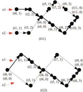
Example 6 The tagged model semantics of the process
ParallelCount(example 2) is a set of behaviors, and two
ex-amples are shown in Fig.5. Similarly, we just consider the external visible signals.
Fig. 5 The tag structures of two possible behaviors of the process
Parallel-Count
Property 2 [12] For all SIGNAL processes, the tagged model semantics is stretch-closed.
Property 1and Property 2 represent that a SIGNAL
pro-cess can be used at different time scales because its semantics is closed for the stretch-equivalence relation.
6
The Proof of the Semantics Equivalence
The trace semantics and the tagged model semantics are very different models, so the equivalence between them
(Theorem-s S2Teqand T2Seq) is established through an intermediate
model. The global idea is sketched in Fig.6.
The intermediate model M is generic and parameterized by:
1) mdom, the domain of M, such as a set of traces, a set of behaviors on a tag structure;
2) mget m x i v, is true in domain m if variable x gets the ith
Fig. 6 Proof’s plan
3) msync m x1x2i1i2, represents whether the variables x1
and x2are synchronized or not at the ith1 non-absent value
and the ith
2 non-absent value respectively.
With these three functions, it is possible to give a seman-tics of SIGNAL, that is Uprocess(M). The difference between the trace semantics and the intermediate model is that the lat-ter just considers non-absent values, while the difference be-tween the tagged model semantics and the intermediate mod-el is that the latter uses a totally ordered set to express logical time. In other words, the intermediate model mixes the fea-tures of both the trace semantics and the tagged model seman-tics. Here, Uprocess(M) is just a general expression, because the domain is unknown. However, we give a general mapping between two intermediate models (M1toM2), and give a ba-sic theorem to prove the equivalence between them (Theorem
TFR12).
The trace semantics and the tagged model semantics are considered as instances of the intermediate model, so we transform them to their instance and prove the equiva-lence (Theorems Ssem_def1, Ssem_def2, Tsem_def1 and
T-sem_def2).
Finally, we consider the relation between the two in-stances. The mapping M1toM2 is refined as m_str2tag and
m_tag2str, and the Theorem TFR12 is reused.
6.1 Intermediate Model
Firstly, we give the definition of the intermediate model.
m-domrepresents the domain of the model. In this model, we
introduce two observers, mget which gives the (finite or in-finite) sequence of values taken by each variable, and msync which defines the synchronization points of any couples of variables.
Record Model : Type : = { mdom : Type ;
mget : mdom → XVar → n a t → V a l u e → Prop ; msync : mdom → XVar → XVar → n a t
→ n a t → Prop } .
Secondly, we define a semantics of SIGNAL using this model, which is a predicate over m ∈ mdom. Here, signal variables x, x1, . . . ,xnare used both in the mathematical
mod-el and the Coq expressions.
Intermediate Model 1 (Instantaneous function)The in-termediate model of the instantaneous function is defined as follows:
Jx := f (x1,· · · , xn)K(m) =
− ∀i ∈ N, ∀v1· · · vnv ∈ V, mget m x1i v1∧ mget m x2i v2
∧ · · · ∧ mget m xni vn∧ mget m x i v
⇒ v = f(v1, . . . ,vn)
− ∀i ∈ N, msync m x1 x i i ∧ msync m x2 x i i ∧ . . .
∧ msync m xnx i i
All signals are synchronous and the ith non-absent
val-ues of each signal satisfy the functional constant v =
f(v1, . . . ,vn).
The Coq expression is given as follows, Uass_T represents the relation between values and Uass_S means all signals are synchronous. Record U a s s i g n m e n t {M} (m: mdom M) I n d e x ( f : ( I n d e x → V a l u e ) → V a l u e ) ( x : XVar ) ( vp : I n d e x → XVar ) : Prop : = { Uass_T : ∀ d v i , ( ∀ p , mget m ( vp p ) i ( d p ) ) → mget m x i v → v = f d ; Uass_S : ∀ p i , msync m ( vp p ) x i i } .
Intermediate Model 2 (Delay)The intermediate model of the delay construct is defined as follows:
Jx := x1$ init cK(m) =
− mget m x0 c
− ∀i ∈ N, ∀v1v2∈V, mget m x1i v1∧ mget m x1(i + 1) v2
⇒ mget m x(i + 1) v1
− ∀i ∈ N, msync m x x1i i
The two signals x and x1 are synchronous. mget m x 0 c
represents the first non-absent value of x is the initial value
c, and the (i + 1)thnon-absent value of x is the ithnon-absent
value of x1, provided it has an (i + 1)thvalue.
Record U d e l a y {M} (m: mdom M) x x1 c : Prop : = { U d e l a y _ 0 : ∀ v , mget m x 0 v → v=c ; U d e l a y _ S : ∀ v1 v2 i , mget m x1 i v1 → mget m x1 ( S i ) v2 → mget m x ( S i ) v1 ; U d e l a y _ s : ∀ i , msync m x x1 i i } .
Intermediate Model 3 (Undersampling)The intermedi-ate model of the undersampling construct is defined as fol-lows:
Jx := x1when x2K(m) =
− ∀i ∈ N, ∀v ∈ V, mget m x i v ⇒
(∃i1i2∈N, msync m x x1i i1∧ msync m x x2i i2
∧ mget m x1i1v ∧ mget m x2i2true)
− ∀i1i2∈N, ∀v ∈ V, msync m x1 x2i1i2
∧ mget m x1i1v ∧ mget m x2i2true
⇒(∃i ∈ N, msync m x x1i i1∧ mget m x i v)
Here, x is defined in the position i if and only if there are two synchronized positions i1and i2at which x1and x2 are
defined, and such as the value of x2 is true. In such a case,
the ithnon-absent value of x is the ith
1 non-absent value of x1.
The Coq expression is given as follows.
Record Uwhen {M} (m: mdom M) x x1 x2 : Prop : = { Uwhen_v : ∀ i v , mget m x i v → ∃ i 1 i 2 , msync m x x1 i i 1 ∧ msync m x x2 i i 2 ∧ mget m x1 i 1 v ∧ ∃ b , mget m x2 i 2 b ∧ i s T r u e b ; Uwhen_v12 : ∀ i 1 i 2 b v , msync m x1 x2 i 1 i 2 → mget m x1 i 1 v → mget m x2 i 2 b → i s T r u e b → ∃ i , msync m x x1 i i 1 ∧ mget m x i v } .
Intermediate Model 4 (Deterministic merging)The in-termediate model of the deterministic merging construct is defined as follows:
Jx := x1de f ault x2K(m) =
− ∀i ∈ N, ∀v ∈ V, mget m x i v ⇒
((∃i1 ∈N, msync m x x1i i1∧ mget m x1i1v)∨
(¬(∃i1∈N, msync m x x1i i1)∧
(∃i2∈N, msync m x x2i i2∧ mget m x2i2v)))
− ∀i i1∈N, ∀v ∈ V, msync m x x1i i1∧ mget m x1i1v
⇒ mget m x i v
− ∀i i2∈N, ∀v ∈ V, (¬(∃i1∈N, msync m x x1i i1)
∧ msync m x x2i i2∧ mget m x2i2v ⇒ mget m x i v
Here, either the ithposition of x is synchronized with some
position of x1, or else it is synchronized with some position
of x2. In both cases, the value of x at the ith position is the
value of the synchronized one.
The Coq expression is given as follows.
Record U d e f a u l t {M} (m: mdom M) x x1 x2 : Prop : = { U d e f a u l t _ v : ∀ i v , mget m x i v → ( ( ∃ i 1 , msync m x x1 i i 1 ∧ mget m x1 i 1 v ) ∨ ( ¬ ( ∃ i 1 , msync m x x1 i i 1 ) ∧ ∃ i 2 , msync m x x2 i i 2 ∧ mget m x2 i 2 v ) ) ; U d e f a u l t _ v 1 : ∀ i i 1 v , msync m x x1 i i 1 → mget m x1 i 1 v → mget m x i v ; U d e f a u l t _ v 2 : ∀ i i 2 v , ( ¬ ( ∃ i 1 , msync m x x1 i i 1 ) → msync m x x2 i i 2 → mget m x2 i 2 v → mget m x i v } .
In addition, we apply these semantics rules to a process to get a complete semantics, that is Uprocess. We also give the semantics of processes composition.
F i x p o i n t U p r o c e s s {M} ( p : P r o c e s s ) (m: mdom M) : Prop : = match p w i t h P a s s I n d f x x i ⇒ U a s s i g n m e n t m I n d f x x i | P d e l a y x x1 c ⇒ U d e l a y m x x1 c | Pwhen x x1 x2 ⇒ Uwhen m x x1 x2 | P d e f a u l t x x1 x2 ⇒ U d e f a u l t m x x1 x2 | P p a r p1 p2 ⇒ U p r o c e s s p1 m ∧ U p r o c e s s p2 m end.
Thirdly, we give a general mapping between two interme-diate models (M1toM2). We use a function s1tos2 to express the mapping from a set of elements of the domain of M1
(de-noted as S1) to a set of elements of the domain of M2. It relies
on a function m2tom1 mapping one element of the domain of
M2 to one element of the domain of M1, such as from one
trace to one behavior on a tag structure.
s1tos2(S1) = {e2∈ mdom(M2)|m2tom1(e2) ∈ S1}
get12and sync12 define the properties of m2tom1, i.e., the
same variable of two models has the same value at the same value index (same mget), and has the same synchronous rela-tions (same msync).
Record M1toM2 M1 M2 : Type : = { m2tom1 : mdom M2 → mdom M1 ; g e t 1 2 : ∀ m2 x i v , mget m2 x i v
↔ mget ( m2tom1 m2 ) x i v ; s y n c 1 2 : ∀ m2 x1 x2 i 1 i 2 ,
msync m2 x1 x2 i 1 i 2
↔ msync ( m2tom1 m2 ) x1 x2 i 1 i 2 ; s 1 t o s 2 : ( mdom M1 → Prop ) → ( mdom M2 → Prop )
: = f u n s 1 ⇒ f u n e2 ⇒ s 1 ( m2tom1 e2 ) } .
Moreover, a basic theorem in which two intermediate models are equivalent is proven. This theorem states that the
transformation of the M2 semantics of a SIGNAL process p is the M1semantics of p. Theorem TFR12 : ∀ M1 M2 ( p : P r o c e s s ) ( t 1 2 : M1toM2 M1 M2) , ∀ ( m2 : mdom M2) , U p r o c e s s (M: =M2) p m2 ↔ s 1 t o s 2 t 1 2 ( U p r o c e s s (M: =M1) p ) m2 .
6.2 The Relation between the Trace Semantics and the In-termediate Model
Notice that, the semantics defined by intermediate model (Uprocess) is generic, because mget and msync are abstract observers. Here, we focus on the relation between the trace semantics and the intermediate model, so we set the domain as a trace. The observers mget and msync also need to be refined, that are trGet and trSync.
The predicate trGet tr i x v is satisfied if the ithnon-absent
value of x is v. I n d u c t i v e t r G e t : T r a c e → n a t → XVar → V a l u e → Prop : = t r g 0 : ∀ x s t t r v , s t x = Val v → t r G e t ( Tr s t t r ) 0 x v | t r g U : ∀ i x s t t r v , s t x = A bs e nc e → t r G e t t r i x v → t r G e t ( Tr s t t r ) i x v | t r g N : ∀ i x s t t r v , s t x , A bs e nc e → t r G e t t r i x v → t r G e t ( Tr s t t r ) ( S i ) x v .
In order to define trSync, we introduce the auxiliary pred-icate trGetp. trGetp tr i x j is satisfied if the ith non-absent
value of x is at the instant j of the trace tr. I n d u c t i v e t r G e t p : T r a c e → n a t → XVar → n a t → Prop : = t r g p 0 : ∀ x s t t r , s t x , A bs e nc e → t r G e t p ( Tr s t t r ) 0 x 0 | t r g p U : ∀ i x s t t r j , s t x = A bs en c e → t r G e t p t r i x j → t r G e t p ( Tr s t t r ) i x ( S j ) | t r g p N : ∀ i x s t t r j , s t x , A bs en c e → t r G e t p t r i x j → t r G e t p ( Tr s t t r ) ( S i ) x ( S j ) . Then, we say that x1and x2synchronize at value index i1
and i2if the ith1 non-absent value of x1and the ith2 non-absent
value of x2occur at the same instant.
D e f i n i t i o n t r S y n c x1 x2 ( t r : T r a c e ) ( i 1 i 2 : n a t ) : Prop : =
∀ j , t r G e t p t r i 1 x1 j ↔ t r G e t p t r i 2 x2 j . We construct the corresponding intermediate model in-stance using the observers trGet and trSync.
D e f i n i t i o n s t r I n s t a n c e : Model : = { | mdom: = T r a c e ; mget t r x i v : = t r G e t t r i x v ; msync t r x1 x2 i 1 i 2 : = t r S y n c x1 x2 t r i 1 i 2 |} .
Finally, we prove the equivalence between the trace se-mantics and its corresponding intermediate model instance. Theorem S s e m _ d e f 1 : ∀ p t r , s t r a c e s ( P r o c e s s 2 S p r o c e s s p ) t r → U p r o c e s s (M: = s t r I n s t a n c e ) p t r . Theorem S s e m _ d e f 2 : ∀ p t r , U p r o c e s s (M: = s t r I n s t a n c e ) p t r → s t r a c e s ( P r o c e s s 2 S p r o c e s s p ) t r .
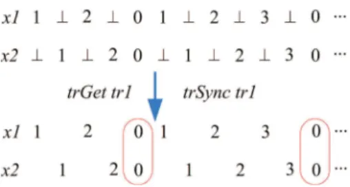
Example 7 We construct the intermediate model instance of the trace tr1 shown in the example 5 (see Fig.7).
Fig. 7 The intermediate model instance of a trace
• trGet tr1 = {(0, x1, 1), (1, x1, 2), (2, x1, 0), (3, x1, 1), . . ., (0, x2, 1), (1, x2, 2), (2, x2, 0), (3, x2, 1), . . . } • trSync tr1 = {(x1, x2, 2, 2), (x1, x2, 6, 6), . . . }
6.3 The Relation between the Tagged Model Semantics and the Intermediate Model
Here, we set the domain as a behavior on a tag structure. The observers mget and msync are refined as tGet and tSync.
In order to define tGet and tSync, we introduce the auxil-iary predicates tGett_from and tGett. tGett s i t is satisfied if the ithtag of the signal s is t.
I n d u c t i v e t G e t t _ f r o m {G} ( t 0 : Tag G ) : T s i g n a l _ f r o m t 0 → n a t → Tag G → Prop : = t g t n 0 : ∀ t 1 h d s t , t = t 1 → t G e t t _ f r o m t 0 ( T n e x t t 0 t 1 h d s ) 0 t | t g t n S : ∀ t 1 h d s i t , t G e t t _ f r o m t 1 s i t → t G e t t _ f r o m t 0 ( T n e x t t 0 t 1 h d s ) ( S i ) t . I n d u c t i v e t G e t t {G} : T s i g n a l G → n a t → Tag G → Prop : = t g t 0 : ∀ d t s , t G e t t ( Tfrom G t d s ) 0 t | t g t S : ∀ t 0 d s i t , t G e t t _ f r o m t 0 s i t → t G e t t ( Tfrom G t 0 d s ) ( S i ) t .
The predicate tGet s i v is satisfied if the value on the ith
I n d u c t i v e t G e t {G} s i v : Prop : = t G e t _ p r f : ∀ t : Tag G, t G e t t s i t
→ t v a l s t v → t G e t s i v .
Then, we say that x1and x2synchronize at tag index i1and
i2if they share the same tag.
I n d u c t i v e t S y n c {G} x1 x2 ( b : T b e h a v i o r G) i 1 i 2 : Prop : =
t S y n c P r f : ( ∀ t , t G e t t ( b x1 ) i 1 t ↔ t G e t t ( b x2 ) i 2 t ) → t S y n c x1 x2 b i 1 i 2 .
We construct the corresponding intermediate model in-stance using the observers tGet and tSync.
D e f i n i t i o n t a g I n s t a n c e G : Model : = { | mdom: = T b e h a v i o r G ; mget b x i v : = t G e t ( b x ) i v ; msync b x1 x2 i 1 i 2 : = t S y n c x1 x2 b i 1 i 2 |} .
Finally, we prove the equivalence between the tagged model semantics and its corresponding intermediate model instance. Theorem Tsem_def1 : ∀ G p b , t b e h a v i o r s ( P r o c e s s 2 T p r o c e s s G p ) b → U p r o c e s s (M: = t a g I n s t a n c e G) p b . Theorem Tsem_def2 : ∀ G p b , U p r o c e s s (M: = t a g I n s t a n c e G) p b → t b e h a v i o r s ( P r o c e s s 2 T p r o c e s s G p ) b .
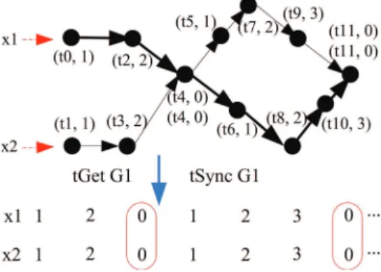
Example 8 We construct the intermediate model instance of the tag structure G1 shown in the example 6 (see Fig.8).
Fig. 8 The intermediate model instance of a tag structure
• tGet G1 = {(x1, 0, 1),(x1, 1, 2), (x1, 2, 0), (x1, 3, 1), . . . , (x2, 0, 1), (x2, 1, 2), (x2, 2, 0), (x2, 3, 1), . . . }
• tSync G1 = {(x1, x2, 2, 2), (x1, x2, 6, 6), . . . }
6.4 The Equivalence between the Trace Semantics and the Tagged Model Semantics
We refine the definition of mapping (M1toM2) as m_str2tag and m_tag2str. In other words, m_str2tag and m_tag2str are defined as instances of M1toM2.
In m_str2tag, the function m2tom1, i.e., from a behavior on a tag structure to a trace, is constructed by a mathemat-ical transformation (transformation 1) which is close to the topological sort algorithm [20], and it is used in the defini-tion of the funcdefini-tion s1tos2, i.e., from the set of traces to a set of behaviors. Lemma m _ s t r 2 t a g : ∀ G, M1toM2 s t r I n s t a n c e ( t a g I n s t a n c e G ) . D e f i n i t i o n S p r o c e s s 2 T p r o c e s s G ( p : S p r o c e s s ) : = { | tdom : = sdom p ; t b e h a v i o r s : = s 1 t o s 2 ( m _ s t r 2 t a g G ) ( s t r a c e s p ) |} .
Transformation 1 Let us consider the mapping from a behavior on a tag structure to a trace. It must visit the tags of each signal following their chain order and must be fair(all the tags of all the signals must be eventually visited). For that, we use a variant of topological sort algorithm and the finiteness of the set signal variables.
• Step0: consider the first tag of each signal, i.e., the tag index on each signal is 0, denoted as the vector of tag
indexes: 0 0 .. . 0 .
• Step1: select any signal such as:
- no other signal will synchronize in the strict future with its current position.
- it has a minimal index compared to indexes of such signals.
• Step2: get the current tag of the chosen signal.
• Step3: add to the target trace the values of the signal variables for that tag, while the values of other signals variables are noted ⊥.
• Step4: increment the index of all the signals of which current tag is the chosen tag, namely their tag index will
be added 1, for example 1 0 .. . 0 .
• Step5: repeat step1, step2, step3 and step4.
The transformation stops if there does not exist any vari-ables with an associated tag at its current tag index. In this
case, the resulting trace is finite. Otherwise, the transforma-tion builds an infinite trace.
Example 9 According to transformation 1, the tag struc-ture G1 in the example 6 can be mapped to a set of traces (different arrangement of values), and the trace tr1 shown in the example 5 belongs to this set (see Fig. 9).
Fig. 9 Mapping from a tag structure to a trace
The tag index on each signal is noted on the tag structure explicitly. The transitions of the vector of tag indexes of tr1 and tr2 are given respectively as follows.
" 0 0 # →" 1 0 # →" 1 1 # →" 2 1 # →" 2 2 # →" 3 3 # →" 4 3 # →" 4 4 # →" 5 4 # →" 5 5 # →" 6 5 # →" 6 6 # → ∅ " 0 0 # →" 1 0 # →" 2 0 # →" 2 1 # →" 2 2 # →" 3 3 # →" 4 3 # →" 4 4 # →" 5 4 # →" 5 5 # →" 6 5 # →" 6 6 # → ∅
In m_tag2str, the function m2tom1, i.e., from a trace to a behavior on a tag structure, is constructed by another math-ematical transformation (transformation 2), and it is used in the definition of the function s1tos2, i.e., from a set of behav-iors to a set of traces.
Lemma m _ t a g 2 s t r : ∀ G, M1toM2 ( t a g I n s t a n c e G) s t r I n s t a n c e . D e f i n i t i o n T p r o c e s s 2 S p r o c e s s G ( p : T p r o c e s s G) : = { | sdom : = tdom p ; s t r a c e s : = s 1 t o s 2 ( m _ t a g 2 s t r G ) ( t b e h a v i o r s p ) |} .
In order to map the infinite traces on the tag structure, we must suppose that infinite chains exist, one of these chains
will be chosen to map all the traces. So, we have the follow-ing hypothesis.
Hypothesis 1 A tag structure always has at least an infi-nite chain.
The Coq definition is given as follows. C o I n d u c t i v e h a s I n f i n i t e C h a i n F r o m {G} ( t : Tag G ) : Type : = NextTag : ∀ t 1 , t @< t 1 → h a s I n f i n i t e C h a i n F r o m t 1 → h a s I n f i n i t e C h a i n F r o m t . I n d u c t i v e h a s I n f i n i t e C h a i n G : Type : = F i r s t T a g : ∀ ( t : Tag G) , h a s I n f i n i t e C h a i n F r o m t → h a s I n f i n i t e C h a i n G . H y p o t h e s i s i n f c h : ∀ G, h a s I n f i n i t e C h a i n G . Transformation 2 Let us consider the mapping from a trace to a behavior on a tag structure. An infinite chain of the target tag structure is noted by the tags {ti| i =0, 1, · · · }
which correspond to instants ( j = 0, 1, · · · ) of the trace. • Step0: start from the first instant of the trace, find the
first position which has non-absent value, if the position cannot be found, then return an empty chain.
• Step1: note the variable-value pair on the corresponding tag of the infinite chain.
• Step2: from the current position, find the next position which has non-absent value, if the position cannot be found, then return the chain which is ended at the current position.
• Step3: repeat Step1 and Step2.
Finally, each signal variable will get a sub-chain.
Example 10 According to transformation 2, the trace tr1 shown in the example 5 is mapped to an infinite chain with non-absent values, which has the same observers tGet and
tSyncwith the tag structure G1 in the example 6 (see Fig.10).
Fig. 10 Mapping from a trace to a tag structure
Finally, we prove the theorems S2Teq and T2Seq based on all the definitions and theorems as above.