Development of a heated multilayer shear sensor

(1)

DEVELOPMENT OF A HEATED MULTILAYER SHEAR SENSOR

by

Todd Jerard Barber

B.S. Aero. Eng., Massachusetts Institute of Technology (1988)

SUBMITTED TO THE DEPARTMENT OF AERONAUTICS & ASTRONAUTICS

IN PARTIAL FULFILLMENT OF THE REQUIREMENTS FOR THE DEGREE OF

MASTER OF SCIENCE in Aeronautics & Astronautics

at the

MASSACHUSETTS INSTITUTE OF TECHNOLOGY

February 1991

Signature of Author ... ..:..:.... ... . ... ...

Departm of Aero tics & Astronautics

S, / ,,October 1990

Certified by ... .. .. .-... ... ... . ...

Alan H. Epstein Professor, A/eronautips & Astronautics

A ccepted by ... .. - ....t- ...0...A...

PHarold Y. Wachman, Chairman Departmental Graduate Committee Department of Aeronautics & Astronautics

MA$SACHUsETTS1STRUTE

OF TECHNlrV(iGY

FEB

19 1991

(2)

DEVELOPMENT OF A HEATED MULTILAYER SHEAR SENSOR

by

TODD JERARD BARBER

Submitted to the Department of Aeronautics & Astronautics February, 1991 in partial fulfillment of the

requirements for the Degree of Master of Science in Aerospace Engineering

ABSTRACT

An experimental study was carried out to test the feasibility of using a double-layer heat transfer gauge for ultimate application in determining the time-resolved behavior of the boundary layer, passage shock, and possible separation point on a transonic compressor rotor blade. In particular, a gauge with equivalent heater and sensor temperatures was tested, to see the effect of cancelling the steady-state heat conduction into the substrate. Tests were performed in a subsonic wind tunnel for steady calibrations and in a shock tube for an unsteady step response. For the steady flow case, the use of a controlled gauge allowed for the calculation of the skin friction over a flat plate. Experimental results agreed with theory within the accuracy of the experiment at all but the lowest sensor overheat ratios. Shock tube predictions for the voltage change of the sensor across the shock were generally good, except for one case tested. In both scenarios, the theoretical model overpredicted the actual sensitivity of the gauge to Mach number.

A new gauge geometry was designed for future compressor testing, with tradeoff studies being performed for the parameters under the control of the experimentalist. In particular, both four-element and ten-four-element gauges were designed specifically with compressor testing as the ultimate application.

Thesis Supervisor: Dr. Alan H. Epstein

(3)

ACKNOWLEDGEMENTS

The list of people who share this accomplishment with me is truly enormous and it is my pleasure to recognize their efforts. First and foremost, I would like to extend my deepest thanks to Professor Alan Epstein for his uncanny experimental talents, his extreme friendliness and approachability, and his faith in my abilities through all the trials and tribulations of an experimental thesis. His patience, understanding, and expertise will not be soon forgotten.

The GTL support staff has eased my journey through graduate life beyond comprehension. The efforts of Viktor Dubrowski, Roy Andrew, Jim Nash, Bob Haimes, and Jerry Guenette have literally saved months of aimless wandering. Karen Hemmick, Holly Rathbun, Nancy Clark, and Diana Park all have been indispensable for the completion of this project. It is with a twinge of sadness that I leave you all.

My fellow students in GTL have truly been an inspiration for over two years now. There are so many who have helped me through, not just in a technical sense. I would like to formally thank Sasi Digavalli, Judy Pinsley, and Pete Silkowski for brightening the interior of 31-256 with their friendship. To Martin Graf, my new friend and successor, I wish to extend a special welcome and a heartfelt thank you for making my last weeks at MIT as pleasant as possible. I offer my deepest respect and thanks to Charlie Haldeman, the one student in GTL who was never too busy to drop his work and solve my problems. To my best friend in the GTL, Tonghuo Shang, I send a mixed message--a happy 'thank you for everything and best wishes for you and your wife' and a sad 'goodbye, buddy....'

The faculty in GTL, both permanent and visiting members, have provided many useful technical hints throughout this project. In particular, I greatly appreciate the efforts of Dr. Edward Greitzer, Dr. Choon S. Tan, Dr. Mike Giles, and Dr. Peter Bryanston-Cross for their timely advice.

Without the wonderful friendships I've enjoyed outside of GTL, my journey through a master's degree would have been much

(4)

more difficult. _{I give a special thanks to Al, Aric, Ella, Emily,} Glenn, Greg, Gus, Iman, Jamie, John, Sam, Steve A., Thomas, Tricia, Venkat, and Will. You are all the best. Notice I listed these alphabetically, absolutely devoid of any favoritism. I'm no dummy--I want to keep my friends. I shall miss all of you so very, very much.

I want to express my deepest gratitude to my family in Kansas. To Mom, Dad, and Lea--thanks for being there for me for eighteen years, helping me to grow into a (more or less) well-adjusted adult. It's too bad MIT has taken all of that away. Just kidding. I love you all very much. Whatever my successes, I take along a part of you.

Finally, I want to send my love across the miles to Lisa, the most special person in my life. Your caring and support through the darkest of days were the one thing that always kept me going. I treasure all of our wonderful memories. Soon we will begin a lifetime of memories together. Oh, and one more thing: Psyche, silly willy...your sugar booger will be there soon!

(5)

LIST OF FIGURES

CHAPTER 2

Figure 2.1:

Figure 2.2: Figure 2.3:

Constant temperature anemometer feedback loop Thin-film heat transfer gauge cross-section

Comparison of gauges and operating modes

CHAPTER 3

Figure 3.1: Normalized unsteady substrate conduction vs. time Figure 3.2: Normalized unsteady substrate conduction vs.

logl 0(time)

Figure 3.3: Normalized unsteady substrate conduction vs. time; effect of the glue layer

Figure 3.4: Normalized unsteady substrate conduction vs. log 10(time); effect of the glue layer

Figure 3.5: Comparison of parallel and series gauge geometries Figure 3.6: Series to parallel gauge voltage ratio vs. number of

resistance elements

Figure 3.7: Sensor voltage vs. normalized shock position; ars =

1.2, laminar flow

Figure 3.8: Sensor voltage vs. normalized shock position; ars = 1.4, laminar flow

Figure 3.9: _{Sensor voltage vs. normalized shock position; ars =} 1.2, turbulent flow

Figure 3.10: Sensor voltage vs. normalized shock position; ars = 1.4, turbulent flow

Figure 3.11: Sensor voltage change vs. temperature ratio: ars = 1.2, laminar flow

Figure 3.12: Sensor voltage change vs. temperature ratio: ars = 1.4, laminar flow

Figure 3.13: Sensor voltage change vs. temperature ratio: ars = 1.2, turbulent flow

(9)

3.14: Sensor voltage change vs. temperature ratio: ars = 1.4, turbulent flow

3.15: Oscillating shock on a multi-element gauge Figure Figure Figure Figure Figure Figure Figure Figure Figure Figure = 1.378 a/square

3.19: Dissipated heat flux vs. overheat ratio

3.20: Dissipated to supplied power ratio vs. gauge resistance; effect of n for fixed tag to element resistance ratio

3.21: Dissipated to supplied power ratio vs. gauge

resistance; effect of tag to element resistance ratio for a fixed n

3.22: Actual [2D] to expected [1D] resistance ratio vs. width to length ratio of rectangular tag

3.23: Plate to element resistance ratio vs. number of elements; material= copper; effect of a of plate material

3.24: Plate to element resistance ratio vs. number of elements; material= gold; effect of a of plate material

3.25: Plate to element resistance ratio vs. number of elements; effect of plate material for a given plate thickness

3.26: Four-element gauge design 3.27: Ten-element gauge design

CHAPTER 4

Figure 4.1: Figure 4.2: Figure 4.3:

Shock tube experimental apparatus Shock tube configuration: before burst

Shock tube configuration: x-t diagram after burst

3.16: Electric power dissipated vs. number ot elements:

= 0.342 2/square

3.17: Electric power dissipated vs. number of elements: = 0.684 a/square

3.18: Electric power dissipated vs. number of elements:

Figure

Figure Figure

(10)

Figure 4.4: Figure 4.5: Figure 4.6: Figure 4.7: Figure Figure Figure Figure Figure Figure Figure 4.8: 4.9: 4.10: 4.11: 4.12: 4.13: 4.14: Figure 4.15: Figure 4.16: Figure 4.17: Figure 4.18: Figure 4.19: Figure 4.20: Figure 4.21: Figure 4.22: Figure 4.23: Figure 4.24:

Shock tube configuration: pressure and temperature profiles with streamwise direction after burst

Maximum data acquisition time vs. shock Mach number

Mean and deviation break pressures for shock tube diaphragm materials

Mean and deviation Mach numbers for shock tube diaphragm materials

Shock speed percentage error vs. Mach number Subsonic wind tunnel experimental apparatus Single-layer sensor shock tube probe support Double-layer sensor shock tube probe support Subsonic wind tunnel flat plate probe support

Flat plate leading edge profile geometry Test material resistance vs. test material temperature

Sensor resistance vs. sensor temperature: the value of as; brass support

Heater resistance vs. heater temperature: the value of ah; brass support

Sensor resistance vs. sensor temperature: the value of as; anodized aluminum support

Heater resistance vs. heater temperature: the value of ah; anodized aluminum support

Subsonic tunnel sensor resistance vs. sensor temperature for as

Subsonic tunnel heater resistance vs. heater temperature for ahl

Subsonic tunnel sensor resistance vs. sensor temperature for as2

Subsonic tunnel heater resistance vs. heater temperature for ah2

Anemometer output voltage vs. sensor cold resistance for a fixed control resistance

Anemometer output voltage vs. sensor overheat ratio resistance for a fixed cold resistance

(11)

Figure 4.25: Sensor to ambient temperature ratio vs. heater to ambient temperature ratio for a passive sensor test Figure 4.26: Balanced-gauge voltage vs. sensor overheat ratio in

zero flow

CHAPTER

5

Figure 5.1: Percentage error vs. error-producing source for a typical flow condition

CHAPTER 6 Figure 6.1: Figure 6.2: Figure 6.3: Figure 6.4: Figure 6.5: Figure 6.6: Figure 6.7: Figure 6.8: Figure 6.9: Figure 6.10: Figure 6.11:

Unsteady voltage traces vs. time: single-layer sensor, low Mach number trials

Unsteady voltage traces vs. time: single-layer sensor, intermediate Mach number trials Unsteady voltage traces vs. time: single-layer

sensor, high Mach number trials

Unsteady voltage traces vs. time: double-layer gauge, low Mach number trials, heater passive, #1 Unsteady voltage traces vs. time: double-layer gauge, intermediate Mach number trials, heater passive, #1

Unsteady voltage traces vs. time: double-layer gauge, high Mach number trials, heater passive, #1 Sensor voltage vs. mass flux: turbulent flow

calibration curves

Sensor voltage vs. mass flux: laminar flow calibration curves

Heater voltage vs. mass flux: turbulent flow calibration curves

Heater voltage vs. mass flux: laminar flow calibration curves

Sensor voltage vs. Mach number: experimental and theoretical output for single-layer sensor, brass probe support

(12)

Figure 6.12: Sensor voltage vs. Mach number: experimental and theoretical output for double-layer gauge, brass probe support, heater passive, #1

Figure 6.13: Sensor voltage vs. Mach number: experimental and theoretical output for double-layer gauge, brass probe support, heater passive, #2

Figure 6.14: Sensor voltage vs. Mach number: experimental and theoretical output for double-layer gauge, brass probe support, heater active

Figure 6.15: Percent difference of theoretical and experimental voltage for a heater active vs. a heater passive case Figure 6.16: Sensor voltage vs. Mach number: experimental and

theoretical output for double-layer gauge, anodized aluminum probe support, heater active, ars = 1.06, t = 0.8 ms

Figure 6.17: Sensor voltage vs. Mach number: experimental and theoretical output for double-layer gauge, anodized aluminum probe support, heater active, ars = 1.08, t = 0.8 ms

Figure 6.20: Sensor voltage vs. Mach number: experimental and theoretical output for double-layer gauge, anodized aluminum probe support, heater active, ars = 1.08, t

= 1.27 ms

(13)

Figure Figure Figure Figure Figure Figure Figure Figure Figure Figure APPENDIX B Figure B.1: Figure B.2: Figure D.1: Figure D.2:

Optimum tag to element resistance ratio vs. number of elements

Optimum element resistance vs. number of elements APPENDIX D

Unsteady voltage traces vs. time: double-layer gauge, low Mach number trials, heater passive, #2 Unsteady voltage traces vs. time: double-layer gauge, intermediate Mach number trials, heater passive, #2

6.23: Experimental to theoretical skin friction ratio

actual mass flux for turbulent flow

6.24: Experimental to theoretical skin friction ratio actual mass flux for laminar flow

6.25: Skin friction coefficient vs. Mach number for turbulent flow: experiment vs. theory

6.26: Skin friction coefficient vs. Mach number for laminar flow: experiment vs. theory

6.27: Experimental to theoretical skin friction ratio true mass flux: ars1 = 1.02, ars2 = 1.04

6.29: Experimental to theoretical skin friction ratio true mass flux: ars = 1.02, ars2 = 1.08

6.32: Experimental to theoretical skin friction ratio true mass flux: arsi = 1.06, ars2 = 1.08

VS. vs. vs. vs. vs. vs. vs. vs.

(14)

Figure D.3: Figure D.4: Figure D.5: Figure D.6: Figure D.7: Figure D.8: Figure D.9: Figure D.10: Figure D.11: Figure D.12: Figure D.13: Figure D.14:

Unsteady voltage traces vs. time: double-layer gauge, high Mach number trials, heater passive, #2 Unsteady voltage traces vs. time: double-layer gauge, low Mach number trials, heater active, brass

support

Unsteady voltage traces vs. time: double-layer gauge, intermediate Mach number trials, heater active, brass support

Unsteady voltage traces vs. time: double-layer gauge, high Mach number trials, heater active, brass support

Unsteady voltage traces vs. time: double-layer gauge, low Mach number trials, heater active,

anodized aluminum support, ars = 1.06

Unsteady voltage traces vs. time: double-layer gauge, intermediate Mach number trials, heater active, anodized aluminum support, ars = 1.06 Unsteady voltage traces vs. time: double-layer gauge, high Mach number trials, heater active, anodized aluminum support, ars = 1.06

Unsteady voltage traces vs. time: double-layer gauge, low Mach number trials, heater active, anodized aluminum support, ars = 1.08

Unsteady voltage traces vs. time: double-layer gauge, intermediate Mach number trials, heater active, anodized aluminum support, ars = 1.08 Unsteady voltage traces vs. time: double-layer

gauge, high Mach number trials, heater active, anodized aluminum support, ars = 1.08

Unsteady voltage traces vs. time: double-layer gauge, low Mach number trials, heater active, anodized aluminum support, ars = 1.11

Unsteady voltage traces vs. time: double-layer gauge, intermediate Mach number trials, heater

(15)

Figure D.15: Unsteady voltage traces vs. time: double-layer gauge, high Mach number trials, heater active, anodized aluminum support, ars = 1.11

(16)

LIST OF TABLES

Table 3.1: Gauge design system parameters for the four-element and ten element gauges

Table C.1: Comparison of predicted and measured shock speeds for the shock tube: shock tube familiarity testing with heavy duty aluminum foil only

Table C.2: Comparison of predicted and measured shock speeds for the shock tube: shock tube familiarity testing with a variety of diaphragm materials

Table C.3: Comparison of predicted and measured shock speeds for the shock tube: diaphragm material testing

Table C.4: Comparison of predicted and measured shock speeds for the shock tube: heat transfer data recorded for a single-layer sensor (#1)

Table C.5: Comparison of predicted and measured shock speeds for the shock tube: heat transfer data recorded for a single-layer sensor (#2)

Table C.6: Comparison of predicted and measured shock speeds for the shock tube: heat transfer data recorded for a homemade double-layer gauge with the heater run passively

Table C.7: Comparison of predicted and measured shock speeds for the shock tube: heat transfer data recorded for a homemade double-layer gauge with the heater run actively

Table C.8: Comparison of predicted and measured shock speeds for the shock tube: heat transfer data recorded for a turbine double-layer gauge on anodized aluminum with the heater run actively; ars = 1.06

Table C.9: Comparison of predicted and measured shock speeds for the shock tube: heat transfer data recorded for a turbine double-layer gauge on anodized aluminum with the heater run actively; ars = 1.08

(17)

Table C.10: Comparison of predicted and measured shock speeds for the shock tube: heat transfer data recorded for a turbine double-layer gauge on anodized aluminum with the heater run actively; ars = 1.11

(18)

CHAPTER 1 BACKGROUND AND INTRODUCTION

A hot-film or hot-wire probe is a useful diagnostic tool for

making steady or time-resolved measurements in a given flow. The hot-film seems particularly well-suited for making measurements in the boundary layer of a rotating compressor (as in a modern gas turbine axial-flow machine) due to its proven technology, ability to withstand centrifugal stresses, absence of interaction with the flow field, high frequency response, and its capacity for spatial resolution. The structure of the boundary layer, possible separation point, and the oblique passage shock on a compressor rotor blade is largely unknown, particularly in an unsteady sense. A correctly designed and calibrated thin-film

gauge may be able to be used to directly verify and measure these phenomena in a compressor test rig. This dictates the design of a thin-film heat flux gauge specifically for that purpose.

In particular, it is postulated [Epstein, Gertz, Owen, and Giles] that vortex shedding in upstream compressor blade wakes drives an observed 15 kHz oscillation of the oblique passage shock. This was inferred from a bimodal velocity histogram from experimental laser anemometry data. A shock oscillation amplitude of 0.5 mm was proposed to explain the observations. It is desired to verify this amplitude and frequency of oscillation for the passage shock directly. The thin-film heat transfer gauge offers the experimentalist a means to do so.

In addition, a low frequency ( 350 Hz) oscillation is inferred in the experimental measurements as well. It is postulated that this is due to an oscillation of a separation point on the suction surface of the rotor blade. Again , thin-film heat transfer technology may

(19)

indirect observations previously made. Also of interest is the location of a possible transition point in the boundary layer on the compressor blade. The success of a computational code (CFD model) for a turbomachine component hinges on knowledge of the correct location of the transition point from laminar to turbulent flow. In short, a well-designed thin-film heat transfer gauge may provide the mean and time-resolved flow structure in a transonic compressor rotor passage.

Such a thin-film gauge would need to be designed with all of the above criteria in mind. In particular, a double-layer multi-element heat transfer gauge has been developed [Epstein, Guenette, Norton, and Yuzhang] that satisfies many of the requirements above. Proof of concept testing and preliminary calibrations may be performed on these readily available gauges. Ultimately, a gauge with a geometry tailored to the application (mapping the unsteady flow structure on a compressor rotor blade) should be designed, calibrated, and tested on a compressor simulation rig. It is the aim of this work to perform experiments on readily available thin-film gauges to obtain predictions for the sensor voltage changes as a function of the flow properties in the test. In particular, steady-state and time-resolved testing should both be performed for a wide variety of flow Mach numbers, controlled gauge temperatures, and operating modes (described subsequently). Theoretical predictions for these output voltage changes should be compared with the actual experimental observations for consistency. In addition, a candidate gauge design for the compressor testing should be presented, after a tradeoff study is performed for the various gauge parameters that are determined by the designer.

(20)

CHAPTER 2 THIN-FILM HEAT TRANSFER GAUGES:

INTRODUCTION AND OPERATION

2.1 INTRODUCTION TO THIN-FILM HEAT TRANSFER GAUGES

The use of single thin-film heat transfer gauges as a flow sensor, via constant temperature anemometry, is a familiar concept [Blackwelder]. The principle of operation is identical to that of a hot-wire anemometer, which is a very popular diagnostic tool. A constant temperature anemometer is an electronic feedback loop that will maintain a resistor (called the "probe" or "gauge") at a certain resistance value set by the operator. There exists an approximately linear relationship between resistance and temperature:

Rh = Rc [1 + a(Tg -To)] (2.1) where Rh is the hot resistance (equal to the control resistance), Rc is the cold resistance (the resistance of the gauge at To), Tg is the gauge operating temperature, To is the ambient or reference

temperature, and a is the coefficient of thermal resistivity of the thin-film material. The ratio of the hot to the cold resistance Rh/Rc is known as the resistive overheat ratio (ar), or the overheat ratio for short. Therefore, a constant temperature anemometer loop fixes a gauge to be at a temperature Tg which is higher than ambient temperature (since ar>l). See Figure 2.1 for a schematic of the anemometer bridge loop employed.

A standard TSI anemometer unit, model 1050A, was throughout testing. In a hot-wire anemometer, the heat provided (via a current) to the gauge is dissipated into the surrounding flow via

(21)

is increased, for example, the convection of heat away from the hot-wire to the flow is increased; therefore, more current needs to be provided to the gauge to maintain it at the elevated temperature Tg. This change can be seen by monitoring the voltage value across the gauge. Since the temperature (and hence resistance) of the gauge is a constant and the current has increased, the voltage value across the gauge will increase accordingly. In fact, if a reasonable relation can be obtained for the forced convection as a function of velocity, it is possible to use the hot-wire anemometer as a velocity meter, since the temperature of the hot wire is known.

The arguments of the preceding paragraph hold for a hot-film anemometer as well, but additional complications exist. In particular, due to the geometric nature of thin-film gauges, forced convection is not the only heat transfer mechanism of importance. A thin-film gauge consists of a thin (approximately 1000

A)

film of metal (in this case, pure nickel) mounted on an insulating layer of kapton (a polyimide material) called a substrate. The kapton thickness is many times greater than that of the thin nickel film. Figure 2.2 represents a schematic of a cross section of a typical gauge (not to scale). Heat conduction into the substrate allows for another means for heat to be transferred from the heated film, and has indeed been observed in practice.

2.2 OPERATING MODES OF THIN-FILM GAUGES

A comparison of the gauges used (in cross-section) and their operating modes can be seen in Figure 2.3. In the case of the shock tube, the test article represents the shock tube probe support. For the single-layer gauge, the kapton is bonded directly to the test article. For the double-layer gauge, the lower resistor (which acts as a heater) is bonded between the kapton and the test article. Since the heater is bonded intimately with the probe support, it is imperative that the probe support be a non-conducting material. This lead to the requirement that the

(22)

aluminum probe support be anodized. In the heater passive mode, the bottom thin-film resistor is not controlled in a constant temperature anemometer loop. This is in contrast to the heater active mode, in which both the sensor and the heater are controlled in separate anemometer loops. Experimental results utilizing these three operating modes will be presented later.

The off-design condition of balancing both the heater and the sensor to different constant temperatures was not investigated. It was determined that such a configuration was not stable, due to the fact that the resistor operating at lower temperature by the anemometer loop would have its temperature increased beyond its operating temperature due to heat conduction from the resistor operating at higher temperature. Once this elevated temperature is realized in the lower temperature resistor, no means can be provided to reduce the temperature of this resistor back to its operating point (i.e., no mechanism exploiting the Peltier effect exists for these standard anemometer units and probes). This is due to the fact that positive current can only be injected into the gauges by the anemometer unit and increases in current correspond to increases in temperature of the resistor.

Control resistances were set on the anemometer unit using both an external 5:1 bridge and the resistance decades, depending on the resistance value of the probe used. Control resistances less than 50 ohms may be set directly with the resistance decades on a 1:1 bridge, while control resistances greater than 50 ohms must be set using the external control resistor feature on the 5:1 bridge. A simple internal rewiring procedure described in the TSI operating manual allows a toggle between these two methods of setting the control resistances. External control resistors are constructed from potentiometers and standard circuit resistors in series. With this design, the overheat ratio can be changed by adjusting the potentiometer. A circuit resistor is used in series with the potentiometer to allow the use of a lower resistance

(23)

potentiometer, which gives better controllability on setting the overheat ratio.

(24)

2.2-CHAPTER 3

THEORETICAL PREDICTIONS FOR UNSTEADY HEAT

TRANSFER AND MULTI-ELEMENT GAUGE DESIGN

3.1 MODELLING THE UNSTEADY SUBSTRATE HEAT CONDUCTION Various models were tried for the cases of non-zero heat conduction into the substrate. A first attempt at modelling this problem was made by assuming that the support was a good thermal conductor and the temperature at the junction between the substrate and probe support was ambient temperature. This lead to substrate conduction values well over three orders of magnitude higher than the convection changes seen across the shock. From this model, the theoretical voltage output change across the shock was predicted to be no more than 20 mV. Actual output voltage changes across the shock were typically 200-300 mV. Clearly, this model is not sufficient to explain the operation of the device. Rather, an unsteady model must be formulated. It is hoped that this model could demonstrate a much lower value for the conduction into the substrate at the time of data acquisition. In all models employed here, it is assumed that the thermal properties within the thin-film gauge itself can be ignored without substantially affecting the output. This is presumed to be a good assumption due to the low thickness of the nickel film (i.e., the film appears thermally transparent due to its size). This is shown to be the case in Appendix A, which solves the steady conduction solution for the case where the thermal properties of the thin-film are not ignored.

The following unsteady heat transfer problem was solved to investigate the time-dependant behavior of the substrate heat conduction:

(25)

a atJ _(3.1)

`1

ax

2 = at

a2_T

2

aT2

K2 "2 = at(3.2)

subject to the following boundary conditions:

1. T1(O,t)= T* [= Ts-To] = constant

2. Tl(8,t)= T2(8,t)

aT

1

aT2

3. k1

ax

(8,t) = k2 x (8,t) 4. T2(0o, t) = 0 5. Tl(x,O)= 0 6. T2(x,O)= 0

Here, k is the thermal conductivity, 8 is the thickness of the

substrate, and K is the thermal diffusivity. The subscript 1 refers

to the kapton layer and the subscript 2 refers to the brass probe

support. This readily solved via Laplace transform techniques. In

particular, it is found that the temperature in the brass support is represented by:

-q2(x+2i8) e-(q l-q2)8

0i

T2(x,t) = T*(1-0) £1 [e 2(x+2i) e i -2iql8]

i=O _.

(3.3)

where q2 and 3 are defined as follows: s

q2 K2 (3.4)

1

(3.5)

with defined below as:

with y defined below as:

(26)

plclk1

Y= p k (3.6)

P2c2k2

In (3.6), p represents the material density and c represents the material specific heat. The individual terms in (3.3) may be evaluated [Carslaw and Jaeger] using the following relation:

£-1 [e 2X] = erfc [] (3.7)

s _L2

where erfc( ) denotes the complimentary error function defined as follows:

z

erfc(z) = 1 - erf(z) = 1 - 2 e-t2d t (3.8)

This is a common function in unsteady heat transfer problems and is rather well tabulated. Applying (3.7) to (3.8), the following is obtained for the final solution for the temperature in the brass layer: oo T2(x,t) = T*(1-3) i erfc [x + 2.9[2.69i + 1]

2-4 i2t

i=O

(3.9)

From this, it is possible to obtain the conduction by differentiation, since in general:

aT

(27)

Since differentiation is a linear operator, the derivative may be moved under the summation sign when applying (3.10) to (3.9). As a final result:

0O

k2 T* (1 I) -(2i+1)2/197t

qcond r[ ie (3.11)

q •2t = i=0

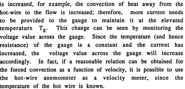
This expression was evaluated numerically by computer. This unsteady conduction, normalized by the steady conduction that would occur if the brass support were at ambient temperature (the previously mentioned steady model conduction), is plotted as a function of time in Figures 3.1 and 3.2. Figure 3.1 represents a plot with a linear time scale, and Figure 3.2 depicts the same plot with the time axis on a logl0 scale. Several features may be noted

in these two figures (particularly Figure 3.2). This time axis represents the time since the anemometers were turned on. Since it is generally many thousands of seconds following this process that the shock tube runs were made, the reduction of the substrate conduction is seen to be striking. This gives much more consistent results when attempting to predict the theoretical voltage jump across a shock, due to the fact that the probe is now much more sensitive to changes in the flow. The peak that occurs after 10 ms in the conduction implies that a thermal wave is propagating from the sensor through the substrate. It is only on time scales of this order that the conduction would severely limit the operation of the heater-passive or single-sensor gauge.

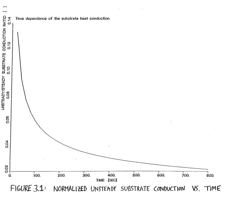
The effect of a finite thickness glue layer on the results presented in Figures 3.1 and 3.2 was numerically investigated.

Assuming that the thermal properties of the glue are similar to that of the kapton (a much more realistic assumption than assuming equivalence with brass), this just increases the value of 8 in the previous calculation. In particular, a 5 gtm glue layer was assumed and the results were recalculated. Presented in Figures 3.3 and Figures 3.4 are the same plots as in Figures 3.1 and 3.2,

(28)

except now the curve representing the scenario with a glue layer are offered for comparison. As can be seen from the graphs, the effect of the glue layer is to slightly move the peak of the conduction graph to the right, towards increased time. This gives slightly higher conduction values after the peak and slightly lower values before the peak for the glue case, consistent with predictions. Since the glue layer thickness is somewhat beyond the control of the experimentalist, it is important to demonstrate that the effect of a glue layer is not a significant contribution to the heat transfer process as modelled here.

3.2 PARALLEL VS. SERIES GAUGES

To completely determine the processes that take place in the boundary layer on a flat plate or compressor blade, spatial resolution of the candidate sensor is an important criterion. In particular, the single resistance bar (such as a DISA sensor) would not allow for good spatial resolution in such an environment, except with a large number of sensors placed in close proximity. Therefore, a multiple-element gauge is desirable for spatial resolution. However, this may adversely effect the signal to noise ratio of the output voltage across the gauge. Two types of multiple-element geometries were investigated; in particular, a parallel (or ladder) geometry and a series (or serpentine) gauge. See Figure 3.5. The use of a series gauge as a hot-film probe has been demonstrated [Epstein, Guenette, Norton, and Yuzhang]. It is desired to compare the voltage across a ladder gauge with that of a serpentine gauge with exactly the same properties. Figure 3.6 represents this relationship, graphing the ladder to serpentine gauge output ratio as a function of the number of resistance elements. This basically scales as the inverse square of the number of resistance elements. Clearly, this dictates that a serpentine pattern be used in the design of a mulitple-element gauge.

(29)

It is desired to know the expected voltage change as a shock wave crosses one element of an n element gauge. This allows the experimentalist to determine, by simply examining the voltage trace from a thin-film heat flux sensor, the presence and the motion of a shock. This is important for attempting to decipher the flow structure on the surface of a transonic compressor blade. Unfortunately, the absolute changes predicted by these models are not physically relevant, since these models were derived using the constant conduction into the substrate model, which has been shown not to be a realistic assumption. However, the shape of the plots will remain unchanged if the unsteady conduction model derived previously is incorporated into the present model. Figures 3.7-3.10 present the sensor voltage as a function of shock position divided by gauge length. Therefore, the leftmost points represent a shock just at one boundary of the gauge and the rightmost points represent the shock after crossing the entire length of the gauge. Two different sensor gauge overheat ratios are presented for both laminar and turbulent flow. Although the change in voltage as the shock propagates is larger in magnitude than is shown here, the nearly linear profile of sensor voltage with shock position over gauge length is expected to be seen, even taking into account the unsteady heat transfer term derived last chapter. Notice that in all cases that higher Mach numbers give larger voltage changes as the shock propagates over the gauge, consistent with intuition. Note also that the predicted value of the absolute voltage level is an increasing function of the overheat ratio, as is expected.

For the case where the heater and sensor are controlled to be at the same temperature in a double-layer gauge (note the distinction between multi-element and multi-layer), the conduction into the substrate can only equal zero if the heater and sensor temperature are balanced exactly. Therefore, it is useful to estimate the decrease in sensor voltage as the temperature difference between the sensor and the heater is increased.

(30)

Figures 3.11-3.14 present the sensor output voltage change across a shock (across all elements of the gauge) as a function of temperature ratio, where the temperature ratio is defined to be the temperature difference between the sensor and the heater normalized by the ambient air temperature. Again, results are presented for both laminar and turbulent flows, with two overheats and three Mach numbers investigated. As before, the absolute voltage level presented here is not correct due to the fact that this model incorporates a steady substrate conduction term. However, the shape of the curve with temperature ratio is consistent with the correct substrate conduction model. In all cases, there is a severe penalty for temperature mismatch between the sensor and the heater. Many of the parameters that determine the proximity of the heater and sensor temperatures are beyond the control of the experimentalist. Good calibrations for a are a necessity, as are carefully prepared control resistors or carefully dialed resistance decade values, depending on the mode of operation of the anemometer units.

3.4 MULTI-LAYER MULTI-ELEMENT GAUGE DESIGN TRADEOFFS 3.4.1 Element spacing

As mentioned above, the spatial resolution of a candidate heat transfer gauge is an important criterion for gauge design. The physical shock oscillation on a transonic compressor blade has been measured to have an amplitude of 0.5 mm. This, however, does not represent the true supersonic interaction length, due to shock wave/boundary layer interactions. In particular, it is desired to know whether the amplitude of shock oscillation is larger or smaller than this supersonic interaction length. Figure 3.15 represents a schematic of this scenario. Correlations can be found for scaling laws for the supersonic interaction domain. It is found that many experimental data points collapse onto one curve, described below:

(31)

L* = 70 60* (Hi - 1)

where L* is the interaction length, 80* is the displacement thickness of the boundary layer, and Hi is the incompressible

shape factor, which is a strong function of the Reynolds number and a rather weak function of the shock Mach number (at least until Ms becomes greater than 1.3, when separation may occur).

For this geometry, it is found that, for the Reynolds numbers encountered on the compressor rotor blade, the supersonic interaction length is roughly 2 mm, or about four times the shock oscillation amplitude. Therefore, the boundaries of the oscillating shock are smeared by the larger interaction region between the oblique shock and the turbulent boundary layer. Hence, providing a spatial resolution less than the shock oscillation amplitude is futile. A design value of 1.00 mm, or 1000 gm was chosen as the distance between adjacent gauge elements (denoted by e). Therefore, the width of the gauge depends only on the the width of the individual resistance elements (5) and the number of resistance elements (n).

3.4.2 Power considerations in gauge sizing

It is an important design criterion that the power supplied by the anemometer be equivalent to the power dissipated in the thin-film gauge. This depends not only on the surface area of the resistance elements, but on the surface area of the tags and leads as well. Tags are the electrical connections between resistance elements (i.e., they are part of the serpentine pattern) and leads are two electrical connections from one side of the heat-flux gauge. In general, the leads for these thin-film gauges are gold-plated to lower their resistance. There is usually no need to plate the tags, as their total resistance is typically small in a serpentine pattern. However, due to the fact that e is so large and that the cold resistance of the gauge is being designed to have a value of 15 Q (to allow standard use on DISA or TSI anemometer units), as well as the power limitations of the anemometer, the tags have a

30.

(32)

substantial resistance in the geometry employed here, so they will need to be gold-plated as well. It was desired to have a gauge that would work even with the failure of the gold-plating, but it was demonstrated that such a gauge cannot be constructed. Therefore, the successful operation of this multi-layer serpentine gauge hinges on the success of the plating process. For a completely non-plated gauge, there is an optimum (i.e., lowest) total tag and lead resistance for a given total resistance. This is demonstrated in Appendix B.

It was decided to select the total tag resistance to be no more than 20% of the total element resistance, since higher tag resistances will reduce the sensitivity of the gauge to flow changes. The effect of changing the parameter 8 is seen in Figures

3.16-3.18, which depict the dissipated electric power as a function

of the number of resistance elements. The three graphs represent three different a values for the gauges, where a is the ohms per square of the gauge. Due to power limitations of the anemometer, a value of 8= 20 pm was selected. This is physically realizable with vacuum sputtering technology. Figure 3.19 presents the correlation for dissipated heat flux as a function of overheat ratio for various materials. For a given overheat ratio and support material for the bonded gauge, this fixes the allowed surface area for the gauge. In particular, Figures 3.20 and 3.21 plot the dissipated to supplied power ratio as a function of gauge cold resistance for different values of n. The horizontal line at one represents the design point. Figure 3.20 shows the effect of the number of resistance elements for a fixed tag to element resistance ratio of 0.1. Figure 3.21 shows the effect of changing the tag to element resistance ratio for a fixed ten-element gauge. However, this is academic, as a value of 0.2 for the tag to element resistance ratio may be too large to assure a sensitive thin-film gauge.

3.4.3 Tag resistance tradeoffs: effects of 2D electrical conduction and plating

(33)

As mentioned before, the resistance of a material is a function of the geometry of the material and a material property known as the resistivity. In particular, for a rectangular conductor of width W, length L, and thickness t [ t << W,L ], the resistance of the plate along its length can be written as:

R =

(3.13)

where p is the resistivity of the material. However, this is only true for the case where current is distributed evenly over each of the sides of width W. The geometry for the thin-film resistance tag is much different than this. Current is injected at one corner of the rectangle and is lead off at an adjacent corner, the length of the side between these two corners being L. Therefore, arbitrarily increasing the width W of a tag element to lower the tag resistance will not work according to (3.13), since the current lines will thin out and therefore less resistance is offered to the total flow of current than would be expected. The analytical solution of the effective resistance of this 2D plate is extremely complex, and numerous attempts at an analytical solution failed. A numerical solution technique, though, can be readily applied. A computer smoothing algorithm was used to solve Laplace's equation for this geometry. Results were obtained for a case with four times fewer grid points, with no noticeable change of the output. This demonstrates that the smoothing algorithm has converged. Presented in Figure 3.22 is a plot of this true resistance, normalized by the resistance expected using (3.13), as a function of the width to length ratio of the tag. This effect clearly demonstrates that the current density rapidly decreases with increasing W, so this is a substantial effect. This model was incorporated into the gauge design model with a noticeable shift in the results. It is clear that this effect is more crucial for higher values of the tag/element resistance ratio. It is also clear that the solution to this problem is a strong function of the ratio of the

(34)

width of the element to the width of the tag (i.e., how much of the rectangle has current entering it and leaving it) This analysis was performed for a tag to element width ratio of 52, but may be performed for an arbitrary tag to element width ratio as well.

The effect of the thickness of the plating material, as well as the choice of plating material, on the resistance of the plating material for different values of n is presented in Figures 3.23-3.25. Figures

3.23 and 3.24 show that there is a severe (i.e., greater than linear)

penalty for choosing higher values of n. However, there is also a sharp decrease in the plate resistance for thicker plates, which may allow for a gauge to be designed with more elements. The desired limit of (Rtag/Relement) < 0.1 may be difficult to obtain in practice for gauges with more than a few elements. Figure 3.25 compares gold and copper as candidates for a plating material, with the plate and thin-film thicknesses set equal. Although copper offers superior performance, the corrosion properties and stability of gold make it a more attractive candidate for plating. There is a practical limit on the thickness of plating that may be allowed. Certainly, a plate thickness of 6000

A

is reasonable, with no significant boundary layer interaction phenomena.

A four-element and a ten-element gauge were designed meeting all the above criteria. Table 3.1 presents the design specifications and the system parameters for both gauges, allowing for either gold or copper plating. The symbols used are defined as follows:

1. 8 = width of the individual gauge element 2. L = length of the individual gauge element

3. e = distance between adjacent gauge elements

4. x = width of individual tag

5. 1 = total length of gauge

6. w = total width of gauge

7. tNi = thickness of thin nickel film

(35)

9. (Pp/PNi) = ratio of resistivities for plate and nickel

10. (RT)cold = total cold gauge resistance

11. (Re)cold = total cold resistance of n elements

12. (Rt)cold = total cold resistance of (n-1) tags

13. (Rt/RT) = ratio of tag to total resistance

Figure 3.26 shows a scale drawing of the four-element gauge, while Figure 3.27 depicts the ten-element gauge. The length of the ten-element gauge is nearly one centimeter, so a spatial map of the surface of a compressor rotor blade may be provided with a minimum amount of difficult and complex instrumentation. These gauges were designed with a stringent requirement that the cold resistance be no more than 15 2 . Very different gauge geometries are possible if the cold resistance of the gauge is allowed to be hundreds or thousands of ohms. This requirement is largely one of familiarity, as this is a typical cold resistance value for a hot wire probe. In addition, with this design, the resistance decades control on the anemometer can be used exclusively to set the overheat ratio, thus eliminating the need for cumbersome homemade control resistors.

(36)

CHAPTER 4

DESCRIPTION OF EXPERIMENTAL APPARATUS

AND TEST GAUGES

4.1 EXPERIMENTAL APPARATUS FOR THE SHOCK TUBE

4.1.1 Introduction and principle of operation

The use of a shock tube offers the experimentalist a relatively simple way to provide a step function in temperature or velocity. This is useful in measuring the unsteady frequency response of a wide variety of flow probes, in this case for a thin-film heat transfer probe. Unsteady flow probe calibrations are also provided via the shock tube. A schematic representation of the GTL shock tube facility is presented in Figure 4.1. This device was constructed with simplicity of operation as the most important criterion. To this end, it was decided to use over-pressure to burst the diaphragm rather than a complex bursting device. This has the disadvantage, of course, of not being able to select the shock Mach number (which is a function of the break pressure) for a given test.

Oil-free air is supplied from the GTL compressor and is controlled via a supply valve. A pressure relief valve (50 psi) is provided for safety purposes. The region to the right of the diaphragm (the "driver" side) in Figure 4.1 is pressurized gradually, to allow for a quasi-equilibrium break of the diaphragm. At this point, the gauge pressure in the driver side is recorded. Upon bursting, a shock wave propagates to the left, into the "driven" side of the shock tube. The action of the shock wave on the pressure transducers will be described subsequently.

(37)

At the moment of rupture, the pressure profile along the length of the shock tube is a step function. Figure 4.2 depicts this configuration, with the moment of rupture arbitrarily called time zero. This facility has the capacity to allow for an evacuation of the driven side of the shock tube, to allow for greater pressure ratios between the driver and driven sides. This allows for arbitrary increases in the shock Mach number, since the Mach number is an increasing function of the break pressure ratio (p4/Pl). However, for these sets of experiments, this vacuum scenario was not employed. Rather, a range of shock Mach numbers were obtained through the use of different diaphragm materials, as explained later.

The physical state of the shock tube somewhat after the burst can best be described with the use of an x-t diagram (see Figure 4.3). All relevant features of the problem can be seen here. At the far left, the shock wave is seen propagating to the left with speed cs. To the immediate right of the shock is the contact

surface, which is moving to the left at speed u2. Physically, the

contact surface represents the discontinuity between the two fluids of different entropy. At the far left is an expansion wave, which propagates to the right into the driver side of the shock tube. The leading expansion wave moves at speed a4, the speed of

sound in the driver gas at burst. The nomenclature for regions (1)-(4) in Figure 4.3 is standard for the shock tube and shall be used extensively here. At the instant in time cited in Figure 4.3, the pressure and temperature profiles along the shock tube are presented in Figure 4.4. The relation between break pressure ratio and Mach number is derived through standard non-stationary shock relations, with the requirement that the pressure and the velocity are continuous between regions (2) and (3). Notice the gradual change of flow properties through the expansion wave, as compared with the (ideally) discontinuous change between regions (1) and (2) and (2) and (3).

4.1.2 Data Acquisition and Triggering Mechanism

(38)

Since the data acquisition time is limited to less than 10 milliseconds for this shock tube (as explained presently), a high-frequency triggering device is clearly an important requirement. High-frequency response static pressure transducers are an excellent choice for a triggering mechanism. Since the pressure increases across a normal shock, as the shock in the shock tube propagates to the left and reaches the rightmost pressure transducer, a step increase in pressure is recorded. This step can be used to trigger a digital oscilloscope to begin recording data from the thin-film heat transfer probe (see Figure 4.1). The thin-film heat transfer probe is located between the two pressure tranducers. By adjusting the time scale on the oscilloscope, the

response of the heat transfer probe to a step in velocity and temperature can be obtained.

Since the distance between the two pressure transducers is known, an experimental value for the shock speed can be obtained by measuring the time delay on the oscilloscope. This experimental shock speed can then be compared to the shock speed predicted by knowing the break pressure ratio, which is also a measured quantity. This gives an internal consistency check. It was found that experimental and predicted shock speeds agreed very well (typically within 1-2 %), but only if the break pressure was approached in a quasi-equilibrium fashion. This is due to the fact that if the pressure is still increasing significantly while the membrane breaks, a well-defined shock front is not established by the time the shock has propagated to the first pressure transducer.

From Figure 4.3, we can see that the data acquisition time is limited by three different constraints. First, the shock wave may reflect from the far left wall and pass over the heat transfer gauge (again). This is called the driven reflection. Second, the contact surface may pass over the heat transfer gauge as it moves left.

(39)

and may interact with the thin-film gauge. This is a driver reflection. The maximum data acquisition time for these three constraints is a function of the shock Mach number, and any one of them may be the important constraint for a given Ms. Plotted

in Figure 2.5 is the maximum data acquisition time as a function

of Ms for the three different constraints mentioned above. It is

seen that the driven reflection is limiting for Ms<1.21, whereas the contact surface is the constraint for Ms>1.21. This is significant, because the Mach number range encountered in testing was

Ms=1.07-1.30.

4.1.3 Selection of diaphragm materials

As mentioned previously, to obtain a range of shock Mach numbers, at least two options are available. The use of vacuum in the driven side was not used due to the difficulty encountered in sealing the driven side from small leaks, particularly at the heat transfer probe attachment junction. Therefore, another option was needed to provide a reasonable Mach number range over which to test the thin-film probes. For a shock tube activated by over-pressure and not a manual bursting device, the only way to obtain a variety of Mach numbers is to use different diaphragm materials. Many possible candidates for diaphragm materials were tested. In particular, four types of Flexel cellophane products were tested, along with two thicknesses of common aluminum foil. Standard aluminum foil, although an attractive diaphragm candidate due to its low burst pressure, was found not to break cleanly enough to allow for a well-defined shock wave to form. This was determined by examining the shape of the pressure pulse as it passed the first pressure transducer. A sharp

rise in pressure signals a well-defined shock wave, whereas a gradual ramp in pressure indicates a shock wave that is getting steeper and is still being formed.

Having eliminated standard aluminum foil, heavy duty aluminum foil was tested. It was found to be an excellent

(40)

diaphragm material, with an intermediate average Mach number (1.21) with very little variance. The four cellophanes tested were Flexel products, with the following Flexel catalog numbers: "K" HB-20, MST, 123 "V" 58P, and 118 "V" 58F. A variety of trials were made with all five of the candidate diaphragm materials. Presented in Figure 4.6 is a plot of the mean break pressure for each of the five diaphragm materials, with one standard deviation shown. Notice that the most repeatable results are obtained with heavy duty aluminum foil. This is a Stop 'n' Shop brand name product, with a thickness of 1.5 mils. Figure 4.7 presents the same data, except now the more physically relevant parameter of shock Mach number is plotted rather than break pressure. It is intended that Figure 4.7 aid future users of the shock tube by offering a standard database for diaphragm material selection. In particular, an experimentalist may choose the membrane that provides the Mach number of interest or may use a variety of

materials to obtain a reasonable Mach number range.

The ultimate proof of concept test for the shock tube comes by comparing the experimental and the theoretical shock speeds. The theoretical shock speed is not truly analytical in an absolute sense because it relies on the measurement of break pressure. However, by comparing the speed implied by the pressure ratio at burst with the speed measured between the two pressure transducers, the degree of applicability of the standard one-dimensional shock tube equations can be determined. Figure 4.8 presents the percentage error in theoretical and experimental shock speeds as a function of Mach number for each shock tube test run. No distinction is made between the different heat transfer gauge conditions utilized, since we are only verifying the correct operation of the shock tube. The excellent agreement between theoretical and experimental shock speeds is clearly seen.

4.2 EXPERIMENTAL APPARATUS FOR THE SUBSONIC WIND

(41)

The shock tube is an ideal diagnostic tool to obtain the unsteady response (at least to a step function) of a thin-film heat transfer gauge. However, it cannot be of assistance in determining the

steady response of one of these probes, nor in obtaining steady

calibrations. The ideal test situation would consist of a subsonic wind tunnel, with provisions for changing the velocity and total temperature of the air stream. Such a facility is readily available and is sketched in Figure 4.9. The test section is split into two separate sections. Both flow speed and total temperature of the flow can be controlled, with a Mach number range for the tunnel from 0.0-0.2 and temperature increase over ambient of up to 40 K possible (for low speeds). Heating of the flow is accomplished through resistive (ohmic) power dissipation far upstream of the test section. The temperature of the airstream was not varied in the experiments performed here.

Flow speed is readily obtained from the manometer board. The static and total pressure at the test section are measured in inches of oil. From Bernoulli's equation, the difference in these two readings reflects the dynamic head of the system. The flow velocity is obtained as follows:

2 po g h sine

v= (4.1)

Pa

where v is the speed of the flow, po is the density of the oil, h is the height difference between the two relevant manometer columns, g is the acceleration due to gravity, 0 is the angle of inclination of the manometer board, and P a is the density of the airstream. A compressible model is used to reduce the data, however, as in the future these concepts may be tested on a steady flow device capable of compressible flow speeds.

4.3 DESCRIPTION OF TEST GAUGES

(42)

4.3.1 Probe supports for the thin film gauges

Several probe supports were constructed to allow the thin-film gauges to be used in the shock tube. A flush-mounting system is used with these gauges, to give minimum disturbance to the flow field of interest. Bonding is accomplished through standard strain-gauge bonding techniques. Both single-layer and double-layer gauges were tested. A double-layer gauge consists of a top thin-film resistor called the sensor, an insulating layer of kapton, and a bottom thin-film resistor called the heater. Figure 4.10 shows a schematic of the single-layer gauge used in shock tube testing. The radius of curvature rc of the right end of the probe support was machined to match the radius of the inner wall of the shock tube (for flush-mounting). An external BNC plug was used for ease of electrical connection with the anemometer units. The probe support was constructed of brass for its desirable thermal and electrical properties. Additionally, a gauge support constructed of anodized aluminum was used for the final set of tests. It was desired to have the same material supporting the gauge, and hence the same thermal properties, as for the flat plate probe support. Figure 4.11 depicts the gauge support for the double-layer gauge. Clearly, four leads are now necessary for the circuitry. An aluminum minibox was used (far left) to facilitate two BNC connectors. For both types of probe supports, the external groove was filled with epoxy to strain-relieve the leads attached to the gauge itself.

The flat plate probe support sketched in the tunnel in Figure 4.9 is shown in detail in Figure 4.12, to scale. The thickness of the anodized aluminum plate is 32 mils. The four square tags in each corner of the flat plate each are equipped with a centered 0.25 inch diameter hole. This is for ease of mounting in the subsonic tunnel as well as for providing a non-critical point of attachment during the anodizing process. As for the shock tube, standard strain-gauge bonding techniques are used to mount the heat transfer gauge to the flat plate. The leads are strain-relieved