Detection of RNA Structural Heterogeneity:
Computational Analysis and Development of Web-based
Tool
by
Sitara C. Persad
Submitted to the Department of Electrical Engineering and Computer Science
in partial fulfillment of the requirements for the degree of
Master of Engineering in Electrical Engineering and Computer Science
at the
MASSACHUSETTS INSTITUTE OF TECHNOLOGY
June 2018
c
○
Sitara C. Persad, MMXVIII. All rights reserved.
The author hereby grants to MIT permission to reproduce and to distribute
publicly paper and electronic copies of this thesis document in whole or in
part in any medium now known or hereafter created.
Author . . . .
Department of Electrical Engineering and Computer Science
May 25, 2018
Certified by. . . .
Prof. Manolis Kellis
Professor, Massachusetts Institute of Technology
Thesis Supervisor
Certified by. . . .
Dr. Silvia Rouskin
Fellow, Whitehead Institute for Biomedical Research
Thesis Supervisor
Accepted by . . . .
Detection of RNA Structural Heterogeneity: Computational
Analysis and Development of Web-based Tool
by
Sitara C. Persad
Submitted to the Department of Electrical Engineering and Computer Science on May 25, 2018, in partial fulfillment of the
requirements for the degree of
Master of Engineering in Electrical Engineering and Computer Science
Abstract
Beyond its function as a messenger molecule in protein formation, the linear sequence on RNA is capable of folding into higher order structures which may interact with other molecules and play key functional roles in the cell. Current methods in characterizing RNA structure via experimental probing are limited to the population average, which obscures structural heterogeneity. This thesis addresses the problem of inferring structural heterogeneity from dimethyl sulphate (DMS) probing data. First, we analysed sequence data to uncover experimental biases and developed simulations for sample structures. We proposed and evaluated machine learning methods in unsupervised learning to infer structural heterogeneity. Secondly, we designed and implemented runDMC, a web platform designed to facilitate the discovery of alternative RNA secondary structures, using in vivo chemical probing data and machine learning clustering methods. runDMC accepts experimental probing data and provides an intuitive, user-friendly interface for discovery of alternative structures. We anticipate that runDMC will facilitate the widespread use of DMS probing and analysis in the biological community, enabling the discovery of more RNA alternative structures. Thesis Supervisor: Prof. Manolis Kellis
Title: Professor, Massachusetts Institute of Technology Thesis Supervisor: Dr. Silvia Rouskin
Acknowledgments
First and foremost, I thank Silvi Rouskin, who welcomed me into her lab and introduced me to the world of research. Without her guidance, wisdom and infectious enthusiasm over the past two and a half years, this thesis would not have been possible. Thank you, Silvi, for everything you have taught me and for the countless opportunities and the endless inspiration you have given me.
Thank you to Professor Manolis Kellis for introducing me to the incredible field of computational biology. I am incredibly grateful to you for your knowledge, enthusiasm and support, and for the opportunities you have given me to delve deeper into the field.
I thank my fellow members of the Rouskin Lab, Paromita, Phil and Margalit, without whom the past few years would not have been nearly as enjoyable. I will fondly remember our discussions, ranging from the biological to the mathematical to the utterly inane. Thanks for making time spent in lab so much fun!
Thank you to Andy Nutter-Upham of the Whitehead IT department, for your assistance navigating the path to deployment and bringing runDMC to life.
To my friends, thank you for the support and laughter that made the past few years some of the best in my life. Finally, I thank my parents, Rambachan and Carmen, and my sister Ashisha. I am incredibly grateful for your unwavering support and continuous encouragement through the process of researching and writing this thesis, throughout my academic career and in each and every one of my life’s endeavours. It is to you that I owe all of my accomplishments.
Contents
1 Introduction 15
1.1 Methods in RNA Structure Prediction . . . 16
1.2 The Problem of Averages . . . 16
1.3 Problem Statement . . . 17
2 Background 19 2.1 Experimental Probing Assays . . . 19
2.2 Clustering Multiple Structures . . . 20
2.2.1 Expectation Maximization . . . 22
3 Simulations 25 3.1 DMS Modification and Reverse Transcription . . . 25
3.2 Simulating Amplification via PCR . . . 29
3.3 Simulating Fragmentation and Sequencing . . . 30
4 Embedded Clustering 33 4.1 Distance-Preserving Embeddings . . . 33
4.2 t-Stochastic Neighbor Embedding . . . 34
4.2.1 Results. . . 35
4.2.2 Signal Boosting . . . 39
4.3 Multidimensional Scaling . . . 41
5 runDMC - A Web Platform for DMS-MapSeq Analysis 45 5.1 User Analysis . . . 46 5.1.1 User Interviews . . . 46 5.1.2 User Classes . . . 49 5.1.3 Interface Goals . . . 50 5.2 Implementation . . . 51 5.2.1 Back-end Infrastructure . . . 51 5.2.2 Front-end Infrastructure . . . 52 5.3 Design . . . 53
5.4 Data Analysis and Results . . . 60
5.4.1 Inputs . . . 60 5.4.2 Sample Statistics . . . 60 5.4.3 Population Average . . . 64 5.4.4 Clustering Results . . . 67 5.4.5 Number of Clusters . . . 68 5.4.6 Structure Visualization . . . 72 5.5 Summary . . . 73 6 Conclusion 75
List of Figures
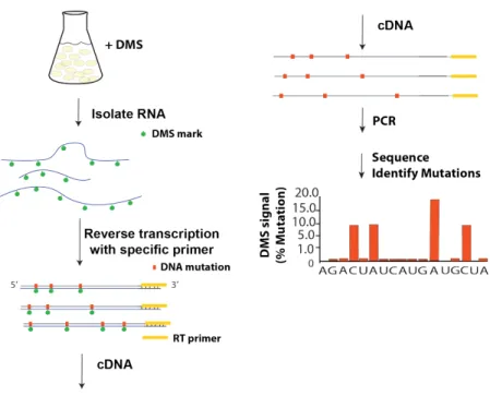
2-1 Experimental Approach for Probing RNA Structure in vivo . . . 20
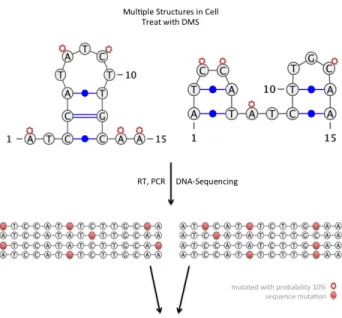
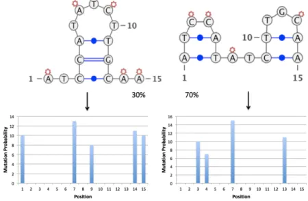
2-2 Population average obscures the signal from individual structures . . . 21
2-3 RNA Structural Heterogeneity can be represented as a mixture of multivariate Bernoulli distributions. . . 22
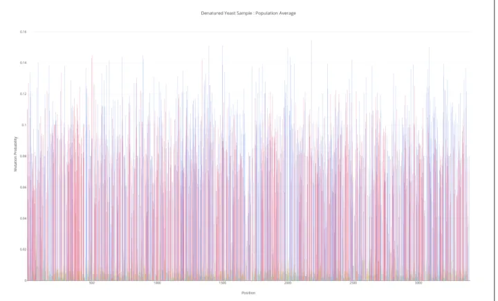
3-1 Reactivity profile for denatured yeast sample. . . 26
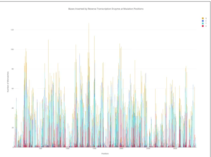
3-2 Distribution of bases induced by RT enzyme at mutated positions. . . 27
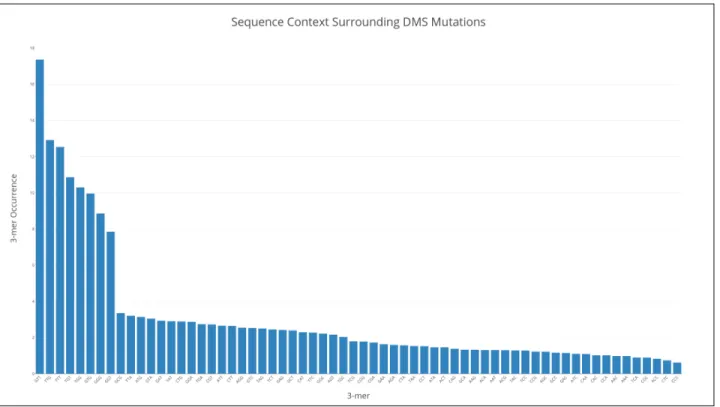
3-3 Sequence context around DMS modifications is highly non-uniform. . . 28
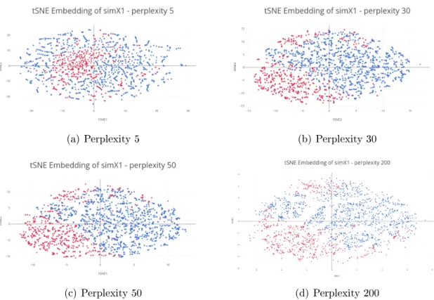
4-1 Simulated structures for the same sequence: simX1-1 (left) and simX1-2 (right) 36 4-2 tSNE Embedding for simX1 for various values of perplexity . . . 36
4-3 Recovery of Clusters in Embedded Space . . . 37
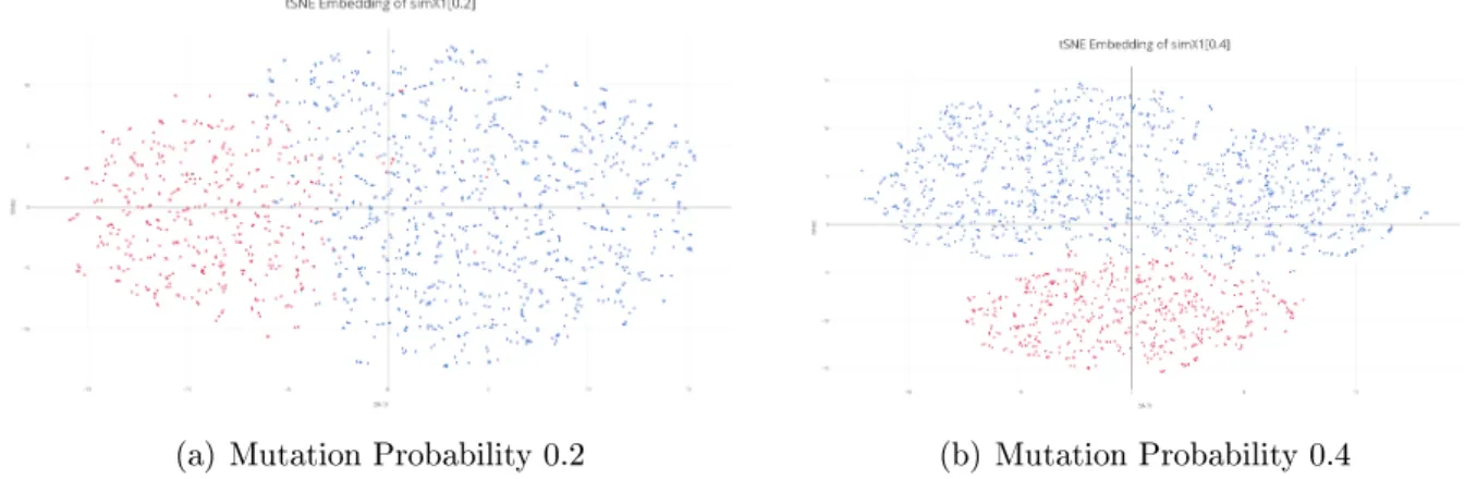
4-4 tSNE Embedding of High Mutation Probability Embeddings . . . 38
4-5 Reads filtered for minimum mutation threshold. . . 39
4-6 Alternative dissimilarity function incorporating nearest neighbor distances. . 40
4-7 tSNE Embedding using Nearest Neighbor Distances . . . 41
4-8 Results of MDS Embedding on simX1. . . 42
5-1 Database Schema for runDMC . . . 52
5-2 The user can view further details about a job . . . 53
5-3 Interface provides streamlined graphical interface for upload and parameter selection . . . 54
5-4 Advanced parameters are available for modification by power users, but otherwise abstracted away . . . 55
5-5 Error messages are provided to highlight mistakes in data entry. . . 56
5-6 A success page confirms valid submission and allows further sample upload. . 56
5-7 All active samples are displayed for the user to access results or sample details. 57
5-8 Details of a sample are provided for easier sample management, along with the facility for free form notes. . . 58
5-9 Results are presented in a report format to easily view all aspects of the analysis 59
5-10 Directory of all results generated by the analysis. . . 59
5-11 The number of data points used in the analysis is displayed, and warnings provided to ensure sufficient sample size. . . 61
5-12 The number of mutations on off-target bases informs the false positive rate. . 62
5-13 The number of mutations per reads can reveal outliers. . . 63
5-14 We generate interactive plots showing sample statistics to help assess experimental success. . . 64
5-15 Bitvector files provide a succinct representation of DMS-MapSeq data for further analysis. . . 65
5-16 The population average highlights positions which are receptive to DMS, and are likely unpaired bases. . . 66
5-17 The number of data points used in the analysis is displayed, and warnings provided to ensure sufficient sample size. . . 68
5-18 The BIC score indicates how well the data fits the model, penalizing the number of free parameters in the model. . . 68
5-19 We display the log-likelihood evolution to visualize whether the algorithm converged. . . 69
5-20 Reactivity profiles allow use to visualize which bases differ in reactivity for different clusters. . . 70
5-21 The correlation between positions in different clusters indicates how cluster similarity. . . 71
5-22 We predict the RNA structure folding using sequence data and experimental constraints. . . 71
5-23 The user can view how well their experimental results agree with the predicted structure. . . 72
List of Tables
3.1 Mutation probability is high for A/C nucleotides. . . 26
3.2 Percentage of each nucleotide induced at mismatch positions. . . 28
4.1 Accuracy of structure recovery for simX1 using differing levels of DMS modification. 38
4.2 Accuracy of structure recovery for simX1 using mutation thresholding. . . . 40
Chapter 1
Introduction
RNA, or ribonucleic acid, is a molecule which plays essential biological roles in all forms of life. Canonically, the principal role of RNA is to act as a messenger molecule, carrying instructions from DNA to control the synthesis of proteins. However, in recent years, scientists have discovered much broader roles of RNA in the cell, such as ribozymes, riboswitches, and small RNAs, some of which control gene expression and play key roles in the function of cellular metabolic networks [15]. These RNAs share the trait of assuming sophisticated functional structures.
Although often thought of as a linear sequence of nucleotides, RNA usually exists in a state where it has folded into higher order structures, defined by base pair interactions (often within a single RNA molecule). These structures are capable of interacting with other molecules and directly catalyzing biochemical reactions. Knowledge of the structure of an RNA molecule can yield critical information on the importance and function of that element. This knowledge has direct biomedical applications, since RNA misfolding has been shown to play a critical role in certain diseases. For example, RNA structure is thought to mediate pre-mRNA splicing and lead to different tau protein versionss [5]. Aberrations in tau splicing regulation are directly linked to several neurodegenerative diseases which lead to dementia.
1.1 Methods in RNA Structure Prediction
As such, the determination of in vivo RNA structure is an important step in understanding structure-function relationships. RNA structure prediction is facilitated by both experimental and computational approaches. Structure prediction algorithms minimize free energy, based on the strength of Watson-Crick base pair interactions, and stacking energies between bases [17]. However, these algorithms do not typically yield accurate results, compared to the gold standard of structures determined by X-ray crystallography, as these prediction algorithms cannot fully capture the effects of three-dimensional interactions and the chemical environment of the cell [4].
In recent years, biologists have used experimental probing assays [16] to infer constraints on bases that are involved in pairing interactions. These constraints can be incorporated in folding algorithms so that predictions are informed by the n cell data or physiological data [2], resulting in accuracies up to 95-100%. However, the field of RNA structure determination is largely limited to characterizing the structure of the population average, which can be grossly misleading.
1.2 The Problem of Averages
The problem with the average comes from the underlying assumption that each member of the population matches the average structure and therefore folds exactly the same way i.e. every RNA molecule with the same sequence will form one stable structure. However, when studied in silico or in solution, RNA sequences often adopt multiple distinct, yet energetically equal, structural conformations, which can have different biological activities. Thus, based on these fundamental biophysical properties of RNA, it is highly likely that RNA structures in vivo are heterogeneous, and the population average structure does not represent any of the underlying structures.
Furthermore, these alternative structures may play different functional roles, so that in order to elucidate the true structure-function relationship, we must be able to detect the presence of alternative structures as well as characterize them. At the Rouskin Lab
in the Whitehead Institute for Biomedical Research, we have been developing an approach for detecting RNA structural heterogeneity using chemical probing followed by Expectation Maximization clustering. This approach has yielded promising results in the field of alternative structure detection. However, it is implemented via a cumbersome and unintuitive command line interface, and the results are difficult to interpret by scientists who are not intimately familiar with the details of the approach, serving as a barrier to entry for many biologists.
1.3 Problem Statement
In order to address these issues, the goal of this project is to explore computational approaches for inferring structural heterogeneity and develop a simple and intuitive web tool for the analysis of chemical probing data to detect RNA structural heterogeneity. We analyze chemical probing data to develop faithful simulations from proposed structures. We propose and evaluate independent methods for detecting alternative structures, and use these simulations to evaluate the developed methods. Finally, we design and build a tool for comprehensive structural analysis, incorporating structure prediction and visualizations directly from experimental data.
This thesis is organized into several chapters. In Chapter 2, we discuss the background work in structure experimental probing techniques, as well as the previous work our lab has done in characterizing structural heterogeneity. In Chapter 3, we analyze DMS sequencing data to verify our assumptions about the process of modification, and use this sequence analysis to develop simulations for alternative structures. In Chapter 4, we propose and evaluate alternative approaches to inferring RNA structural heterogeneity, using the simulations generated in the previous chapter. In Chapter 5, we design and implement a web tool for analysis of RNA structure and structural heterogeneity. In Chapter 6, we summarize the results and contributions of this thesis.
Chapter 2
Background
In this chapter, we look at an overview of existing techniques relevant to this thesis, from the fields of computational and experimental biology. We first discuss the experimental probing work upon which this thesis relies, followed by the computational foundations of clustering and metagenomic assembly.
2.1 Experimental Probing Assays
At the Rouskin Lab in the Whitehead Institute we developed DMS MapSeq, a chemical assay for analysing RNA structure. We use Dimethyl Sulfate (DMS), a small molecule, to experimentally probe RNA structure, either in vitro or in vivo using both a targeted and genome-wide approach. DMS enters cells rapidly and is highly reactive with unpaired adenine and cytosine nucleotides accessible to the solvent but is unreactive with bases engaged in Watson-Crick pairing [16].
We use a special enzyme (TGIRT [10]) to perform reverse-transcription (RT). When this RT enzyme encounters a DMS modification, it will substitute a random base on the reverse-transcribed DNA, which can subsequently be sequenced. We can align these sequences to a reference genome in order to infer the positions of mutations, and, hence, the positions of open bases in the RNA structure. This experimental approach is highlighted in Figure2-1. This approach works well in generating folding constraints in the case where all RNA molecules of the same sequence are folded similarly. However, many RNA molecules are
Figure 2-1: Experimental Approach for Probing RNA Structure in vivo
known to exist in an equilibrium of multiple stable structures simultaneously. In such cases, the population average can be utterly misleading. Figure 2-2 illustrates one such scenario where identifying sequences at the population level provides some insight into RNA structure, but obscures the individual structures. In Section 2.2, we discuss previous work done on separating these structures to infer RNA structural heterogeneity (Rouskin et al, Manuscript In Preparation).
2.2 Clustering Multiple Structures
Recall the process by which DMS induces mismatches, or mutations, on a read. A mutation occurs probabilistically where an open A/C base is present. We can consider each structure, then, to be a probability distribution over mutation positions - open A/C positions will have a relatively higher probability of mutation than other positions.
Suppose then, that we are interested in a region of length 𝐿. Then, for every base position 𝑏𝑖, it has a certain probability, P(𝑏𝑖 = 1), of being mutated, depending on whether
it is an open position, as well as ambient environmental conditions within the cell. We model each position as a Bernoulli random variable, and so a region of length 𝑛 is a multivariate
Figure 2-2: Population average obscures the signal from individual structures
Bernoulli random model (Figure2-3). The set of RNA in the cell, can then be considered as a mixture of such distributions.
Therefore, each read can be considered as a sample drawn from the distribution associated with its true structure. As such, we reformulate each DNA sequence read as a bit vector, where a value ‘0’ corresponds to ‘no mutation’ and a value of ‘1’ corresponds to ‘mutation’. For a given sample, we will generally have on the order of hundreds of thousands of DNA sequence reads converted to bit vectors.
We can then use the Expectation Maximization algorithm to iteratively learn the mixture proportions and probability distribution over bases for each cluster, for some pre-defined number of clusters.
Figure 2-3: RNA Structural Heterogeneity can be represented as a mixture of multivariate Bernoulli distributions.
2.2.1 Expectation Maximization
The Expectation Maximization (EM) Algorithm [3] is an iterative algorithm which finds the best estimate for the parameters of a model that depends on hidden latent variables. In clustering applications, these latent variables are typically the ’true’ membership of each point to each cluster. The EM algorithm optimizes the likelihood of the model parameters, given the set of data. In our case, the model and model parameters are the mutation probabilities on each base in each cluster. Each iteration of Expectation-Maximization performs two steps: the expectation (E) step and the maximization (M) step.
The E step probabilistically assigns reads to clusters and computes the expected likelihood using the current parameters of the model. As described above, each read is reformulated as a sequence of length 𝑙 of 1’s (mutations) and 0’s (wild type bases). The reactivity profile for each cluster, 𝜇(𝑘) is vector of probabilities of length 𝑛 where 𝜇(𝑘)
𝑖 represents the probability
that, for a read belonging to cluster 𝑘, the base at position 𝑖 will be mutated, or P(𝑏𝑖 = 1) =
𝜇𝑖.
We define the proportion of reads belonging to cluster 𝑘 as 𝜋𝑘. These are the mixing
proportions of the model.
as the product of observing each base under the model parameters: P(𝑅𝑒𝑎𝑑|𝜇, 𝜋) = 𝐾 ∑︁ 𝑘=1 𝜋𝑘P(𝑅𝑒𝑎𝑑|𝜇(𝑘)) = 𝐾 ∑︁ 𝑘=1 𝜋𝑘 𝐿 ∏︁ 𝑖=1 P(𝑏𝑖|𝜇(𝑘)) = 𝐾 ∑︁ 𝑘=1 𝜋𝑘 𝐿 ∏︁ 𝑖=1 (𝜇(𝑘)𝑖 )𝑏1(1 − 𝜇(𝑘) 𝑖 ) (1−𝑏𝑖)
For a sample of 𝑁 reads, we compute:
P(𝐷𝑎𝑡𝑎|𝜇, 𝜋) =
𝑁
∏︁
𝑗=1
P(𝑅𝑒𝑎𝑑𝑖|𝜇, 𝜋)
Since the log(𝑥) is increasing in 𝑥, we can equivalently optimize the log-likelihood, log P(𝐷𝑎𝑡𝑎|𝜇, 𝜋) and optimize it with respect to parameters 𝜇 and 𝜋. Optimizing over the log-likelihood allows us to avoid numerical precision errors as well as have a more well-scaled gradient for optimization.
The M step computes the parameters which maximize the log-likelihood function found in the E step. The new parameters are used to update the latent variables in the model, the assignments of points to clusters. These steps are then repeated, until the algorithm converges to a maximum likelihood.
The EM algorithm converges at a point where the derivative of the likelihood is close to zero, that is either a saddle point or a maximal value. There is, however, no guarantee that the point is a global maximum, and indeed the solution derived may not be the globally optimal solution. This issue is alleviated by running the EM algorithm from multiple random initial points, so that at least one run will escape the local maximum and achieve a higher likelihood.
Chapter 3
Simulations
In the absence of biological data with ground truth labels, we create simulated data to test the performance of each approach. In this section, we describe the simulation of this data, along with the simplifying assumptions made.
Given a sequence and corresponding RNA structure, the simulation steps roughly follow the experimental workflow as follows:
1. Simulate treatment of whole molecules using dimethyl sulphate (DMS). Probabilistically induce modifications and RT-induced DNA mutations at these positions.
2. Simulate the polymerase chain reaction (PCR) by naively replicating molecules at random until we have the specified number of duplicated molecules
3. Simulate the random fragmentation of these molecules and subsequent size selection of the fragments for sequencing. Simulate the random sub-sampling of molecules before sampling.
In the following sections, we outline the specific methods and parameters used to produce these simulations.
3.1 DMS Modification and Reverse Transcription
DMS modification is achieved when dimethyl sulphate is introduced into a sample of (folded) RNA molecules, and induces chemical modifications at accessible adenosine or cytosine
(A/C) nucleotides. In order for a base to be accessible it must be both unpaired as well unblocked in three dimensional space.
When DMS encounters an accessible base, it will induce a chemical modification at that base, with some probability, 𝑑𝑚𝑠𝑃 𝑟𝑜𝑏. This probability depends on the concentration of DMS introduced. However, to a first approximation, we will estimate this probability from the population average of a genome-wide denatured sample of yeast containing 100000 reads (Figure 3-1). Mutations on ’A’ are shown in red, ’C’ in blue, ’G’ in yellow and ’T’ in turquoise. The denatured sample is necessarily unstructured, so all A/C bases are accessible. The average probability of mutation on A/C bases was 0.081 ± 0.027. (Table 3.1).
Base Mutation Probability Standard Deviation
A 0.0740 0.0244
T 0.0031 0.0052
C 0.0907 0.0266
G 0.0051 0.0047
Table 3.1: Mutation probability is high for A/C nucleotides.
In order to convert this modified RNA to DNA, we use a special enzyme, TGIRT enzyme for reverse transcription. This reverse transcription (RT) enzyme reads the modified RNA and inserts another nucleotide at this position, theoretically at random. In order to estimate the probability of each base being inserted, we again examine the denatured yeast sample to compute the probability of each base being introduced at a modified A/C base (Figure
3-2). This estimate provides a method for simulating how bases are mutated, denoted by 𝑚𝑢𝑡𝑎𝑡𝑒𝐵𝑎𝑠𝑒() in the pseudocode below.
Figure 3-2: Distribution of bases induced by RT enzyme at mutated positions.
These mutations are summarized in Table3.2. For the most part, the inserted nucleotide is near random (33%). However, original ’A’ nucleotides show a distinct increase in the percentage of ’T’s introduced, and original ’G’ nucleotides show a distinct increase in the percentage of ’A’s introduced.
Original Base A Inserted T Inserted C Inserted G Inserted
A - 69.4 13.2 17.4
T 25.3 - 31.4 43.3
C 38.7 38.5 - 22.8
G 54.5 29.7 15.9
-Table 3.2: Percentage of each nucleotide induced at mismatch positions.
Finally, we know that DMS should only be modifying A/C bases, but we do observe signal on G/T bases. We estimate the false positive rate (FPR) based on the signal of these bases, which allows us to model the noise inherent in the experimental process, which may be introduced during the DMS modification or RT stage of the experiment. The average signal on G/T bases was found to be 0.004 ± 0.005.
The naive assumption is that the probability of a base being modified or mutated is unaffected by the surrounding sequence context. In order to test this assumption, we examine k-mer frequencies around modified A/C bases in the denatured yeast sample, as shown in Figure 3-3.
Figure 3-3: Sequence context around DMS modifications is highly non-uniform.
normalize with respect to the number of k-mer occurrences in the sequence, to account for certain k-mers which may by chance occur more often in the sequence. In contrast to what we expect, we observe a highly non-uniform distribution of k-mers both before modified positions, suggesting that the modification of accessible positions is not in fact random. We account for this by modifying the probability of inserting a DMS modification based on the sequence context immediately preceding. We use k-mer size three, since this is the stretch of bases that the RT enzyme holds on to while traversing the RNA.
We use this sequence analysis to inform our parameters used in simulating DMS data. This overall process is described in Algorithm1.
Data:
𝑆𝑒𝑞𝑢𝑒𝑛𝑐𝑒 - nucleotides comprising the linear RNA sequence
𝑆𝑡𝑟𝑢𝑐𝑡𝑢𝑟𝑒 - dot-bracket string indicating the base pairs in an RNA structure 𝑛𝑀 𝑜𝑙𝑒𝑐𝑢𝑙𝑒𝑠 - the number of molecules to be simulated
Result:
𝑚𝑜𝑙𝑒𝑐𝑢𝑙𝑒𝑠 - array of molecules with mismatches induced at DMS modified positions begin 𝑚𝑜𝑙𝑒𝑐𝑢𝑙𝑒𝑠 ←− [] for molecule ∈ 𝑛𝑀𝑜𝑙𝑒𝑐𝑢𝑙𝑒𝑠 do 𝑚𝑜𝑙𝑒𝑐𝑢𝑙𝑒 ←− [] for (𝑖, 𝑝𝑜𝑠) ∈ 𝑆𝑡𝑟𝑢𝑐𝑡𝑢𝑟𝑒 do base ←− Sequence[i]
if isOpen(base) & Mutate(dmsPprob) || insertFalsePositive(FPR) then if sequenceContextProb(Sequence[i-3:i]) then base ←− MutateBase(base) end end molecule.add(base) end molecules.add(molecule) end end
Algorithm 1: DMS Modification and RT Mismatch Simulation
3.2 Simulating Amplification via PCR
We assume a simple model of PCR amplication where a random molecule is selected and duplicated. This simplifying assumption does not, however, entirely ring true in experimental
settings For example, it neglects the effects of preferential amplication, where the frequency of a few molecules grows exponentially so that the final distribution of molecule proportions does not accurately reflect the initial distribution. Another experimental issue which we do not replicate is the formation of chimeras, where molecules may break and reattach incorrectly, so that it is a hybrid of multiple original molecules. For the sake of simplicity we ignore these effects, although they may be incorporated in further works. The procedure used for the simulations in this work is described in Algorithm 2.
Data:
𝑀 𝑜𝑙𝑒𝑐𝑢𝑙𝑒𝑠 - array of molecules with mismatches induced at DMS modified positions 𝑆𝑡𝑟𝑢𝑐𝑡𝑢𝑟𝑒 - dot-bracket string indicating the base pairs in an RNA structure
𝑚𝑎𝑥𝑀 𝑜𝑙𝑒𝑐𝑢𝑙𝑒𝑠 - the maximum number of molecules after PCR duplication Result:
𝑀 𝑜𝑙𝑒𝑐𝑢𝑙𝑒𝑠 - array of duplicated molecules based on output of PCR begin
while 𝑀𝑜𝑙𝑒𝑐𝑢𝑙𝑒𝑠.𝑙𝑒𝑛𝑔𝑡ℎ < 𝑚𝑎𝑥𝑀𝑜𝑙𝑒𝑐𝑢𝑙𝑒𝑠) do
duplicate ←− chooseRandom(Molecules) Molecules.add(duplicated) end
end
Algorithm 2: PCR Amplification
3.3 Simulating Fragmentation and Sequencing
The final step in the experimental pipeline is to fragment these whole molecules in preparation for paired-end sequencing, which can accommodate reads of length 600 nucleotides (nt) at most. Therefore, before sequencing the PCR products, they must be fragmented and size selected to a certain range. We simulate the fragmentation of PCR products by choosing two random points to break up the PCR product and then select all resulting fragments within the appropriate size. Experimentally, this range is typically 500-600nt.
We assume that fragmentation is random, as previous studies [12] have found that DNA fragmentation by sonication usually results in uniform capture. However, we do not experimentally test this assumption. Gross violations of this assumption can be detected by examining the read coverage over the region of interest and ensuring uniform coverage.
standard for downstream sequence analysis. Data:
𝑀 𝑜𝑙𝑒𝑐𝑢𝑙𝑒𝑠 - PCR products containing amplified molecules Result:
𝑓 𝑜𝑟𝑤𝑎𝑟𝑑𝐹 𝑎𝑠𝑡𝑎, 𝑟𝑒𝑣𝑒𝑟𝑠𝑒𝐹 𝑎𝑠𝑡𝑎 - Fasta files containing paired end sequencing reads. begin
forwardFasta ←− [ ] reverseFasta ←− [ ]
for molecule ∈ Molecules do
fragments ←− breakRandom(molecule) fragments ←− validLength(fragments) for fragment ∈ fragments do
forwardFasta.add(𝑓𝑜𝑟𝑤𝑎𝑟𝑑𝑆𝑒𝑞𝑢𝑒𝑛𝑐𝑒(𝑓𝑟𝑎𝑔𝑚𝑒𝑛𝑡)) reverseFasta.add(𝑟𝑒𝑣𝑒𝑟𝑠𝑒𝑆𝑒𝑞𝑢𝑒𝑛𝑐𝑒(𝑓𝑟𝑎𝑔𝑚𝑒𝑛𝑡)) end
end end
Chapter 4
Embedded Clustering
At the Rouskin Lab, we have implemented Expectation Maximization clustering (Manuscript In Preparation) to detect RNA structural heterogeneity, as discussed in Chapter 2. One shortcoming of the EM approach to clustering RNA structures in high dimensions is that the number of clusters is unknown and must be specified, or inferred by running the algorithm repeatedly and determining the number of clusters using the Bayesian Information Criterion (BIC score) [13]. Running the EM algorithm multiple times is computationally intensive. Furthermore, interpreting the BIC score is unintuitive to experimentalists, unlike using low-dimensional representations which allow us to visualize the data to select the number of clusters. Such low dimensional embeddings would provide more confidence for biologists to determine the number of structures and interpret the structural heterogeneity.
We now investigate alternative clustering approaches to address the weaknesses of the Expectation Maximization (EM) approach, as well as to provide independent validation of the results obtained by the EM method. Thus, we explore several algorithms for low-dimensional representation to determine whether they can detect alternative structures from simulated and experimental DMS probing data.
4.1 Distance-Preserving Embeddings
Alternative structures contain distinct patterns of mutations, corresponding to the open bases in that structure. For each read belonging to a given structure, a subset of these
positions will be mutated. The size of this subset relative to the number of modifiable positions depends on mutation probability which can be controlled, up to a certain level, by the DMS concentration used experimentally. As such, we expect that reads generated by the same structure will contain overlapping mutations. If we formulate reads as a ’0’ where no mutation occurs and ’1’ where a mutation occurs, then we can compute the Hamming distance between reads, which tells us the number of positions that differ between the two reads. This distance should be smaller for reads belonging to the same cluster, and therefore these reads should be neighbors in high dimensional space. We can use this fact to explore distance-preserving embeddings for visualizing RNA structures in low dimension.
We describe two approaches for low dimensional representation that aim to preserve distances between points. We begin by describing these algorithms and then present the results of their performance on our sample datasets.
4.2 t-Stochastic Neighbor Embedding
t-Distributed Stochastic Neighbor Embedding (t-SNE)[9] is a probabilistic approach to low dimensional embedding. Objects are placed in low dimension to preserve neighbors. That is, points that are close in high dimensional space will be close in low dimensional space as well. In order to avoid over-crowding, t-SNE uses a t-distribution over the points in the low dimensional space.
The general method by which objects are embedded is as follows:
1. Create a dissimilarity matrix, D, for each object. A dissimilarity matrix is more flexible than a distance matrix, and only requires the following conditions:
∙ 𝐷𝑖𝑖= 0
∙ 𝐷𝑖𝑗 ≥ 0
∙ 𝐷𝑖𝑗 = 𝐷𝑗𝑖
neighbor 𝑝𝑖𝑗 = exp(−𝐷2 𝑖𝑗) ∑︀ 𝑘̸=𝑙exp(−𝐷 2 𝑘𝑙)
3. For each object 𝑦𝑖 in low dimensional space, compute the probability that 𝑦𝑗 is its
neighbor, using a student’s t-Distribution.
𝑞𝑖𝑗 =
(1 + ‖𝑦𝑖 − 𝑦𝑗‖22) −1
∑︀
𝑘̸=𝑙(1 + ‖𝑦𝑖− 𝑦𝑗‖22)−1
4. Minimize the KL-divergence
𝐾𝐿(𝑃 ‖𝑄) =∑︁
𝑖̸=𝑗
𝑝𝑖𝑗log
𝑝𝑖𝑗
𝑞𝑖𝑗
This is a non-convex optimization problem, and is typically solved using gradient descent. As such, every time t-SNE is run, the algorithm may converge to a different solution.
4.2.1 Results
We evaluate the performance of t-SNE on simulated data, described in Section 3. We first test these approaches on a small, simple structure and then expand our results to more realistic structures.
simX1
We first generate simulations for a small molecule shown in Figure 4-1, which can be sequenced entirely using paired-end or single-end sequencing. This toy molecule has highly distinct structures, so the set of candidate mutable positions (open A/C) bases for each structure is reasonably distinct.
We generate simulated data containing 10,000 reads with a DMS mutation probability 0.10 for this small structure which adopts very distinct conformations, mixing them in a ratio of 70:30, (simX1-1:simX1-2).
Figure 4-1: Simulated structures for the same sequence: simX1-1 (left) and simX1-2 (right)
Perplexity
t-SNE employs a tune-able parameter, the perplexity, which affects how local and global structure is balanced. We run t-SNE on this data, using different values for the perplexity, to observe how well the data separates.
(a) Perplexity 5 (b) Perplexity 30
(c) Perplexity 50 (d) Perplexity 200
Figure 4-2: tSNE Embedding for simX1 for various values of perplexity
We observe that with perplexity 30 and 50, points from the same structure are embedded close together. However, using lower values of perplexity results in poor separation, while higher values begin to create the appearance of clusters which do not exist. Therefore, we
use perplexity values in the range of 30 to 50.
We perform hierarchical clustering as well as expectation maximization using a Gaussian Mixture Model (GMM) in the embedded space to determine how accurately we can cluster the embedded data (Figure 4-3).
(a) Labels Generated by Hierarchical Clustering (b) Labels Generated by GMM EM Clustering
(c) Ground truth labels
Figure 4-3: Recovery of Clusters in Embedded Space
In the embedded space, the clusters could not be recovered accurately. Both hierarchical clustering and GMM EM Clustering fail to accurately recover the initial clusters, achieving AUROC scores of 0.74 and 0.83 respectively. AUROC, or Area Under the Receiver Operating Characteristic curve plots the True Positive Rate versus the False Positive Rate, and computes the area under the curve. A random classifier achieves an AUROC score of 0.5.
Furthermore, under these perplexity values, the number of clusters could not be distinguished using these embeddings if the labels were unknown. In order to use embedding for visualization of structures, these clusters need to be more well separated. The embedded points may not be well separated because the distance between points in different clusters is not sufficiently high. We examine this hypothesis by simulating data with higher DMS mutation probability.
Increased Mutation Probability
We explore the performance of tSNE using high mutation probabilities, in order to determine whether the critical factor in separating structures is the low DMS mutation rate. We experiment with various values of perplexity, and find performance to be robust to perplexity values between 30 and 50. We generate simulations of simX1 using DMS mutation probability 0.2, 0.3 and 0.4, referred to as simX1[0.2], simX1[0.3] and simX1[0.4], respectively.
(a) Mutation Probability 0.2 (b) Mutation Probability 0.4
Figure 4-4: tSNE Embedding of High Mutation Probability Embeddings
We observe that at high signal levels, such as mutation probability 0.3 - 0.4, we can clearly see distinct structures. We apply our clutering algorithms to these sets of data, and observe increased accuracy in structure recovery for mutation probabilities above 0.3, as shown in Table 4.1.
Hierarchical Clustering EM Clustering with GMM
Sample Accuracy AUROC Accuracy AUROC
simX1[0.1] 0.71 0.74 0.8 0.83
simX1[0.2] 0.81 0.85 0.85 0.89
simX1[0.3] 0.95 0.96 0.95 0.92
simX1[0.4] 0.98 0.98 0.96 0.98
Table 4.1: Accuracy of structure recovery for simX1 using differing levels of DMS modification.
However, these levels of DMS modification are not achievable experimentally - we typically observe maximum mutation levels of approximately 0.15. Thus, we must explore methods for boosting experimental signal computationally.
4.2.2 Signal Boosting
We return to simulations using realistic levels of DMS mutation probability, such as simX1[0.1]. Our previous results show that in our embeddings, points belonging to the same structure in simX1 are generally close to each other in low dimensional space. However, points in different structures are not sufficiently separated. This problem is due to the fact that there is insufficient distance between points in different clusters, potentially due to the fact that there are not sufficient mutations on a given read. This explains why high mutation levels lead to improved separation, as the reads generated from these simulations have more mutations per read on average.
One possibility, then, for improving the separation between structures in embedded space is to discard reads with few mutations. We evaluate this approach in the following section.
Mutation Thresholding
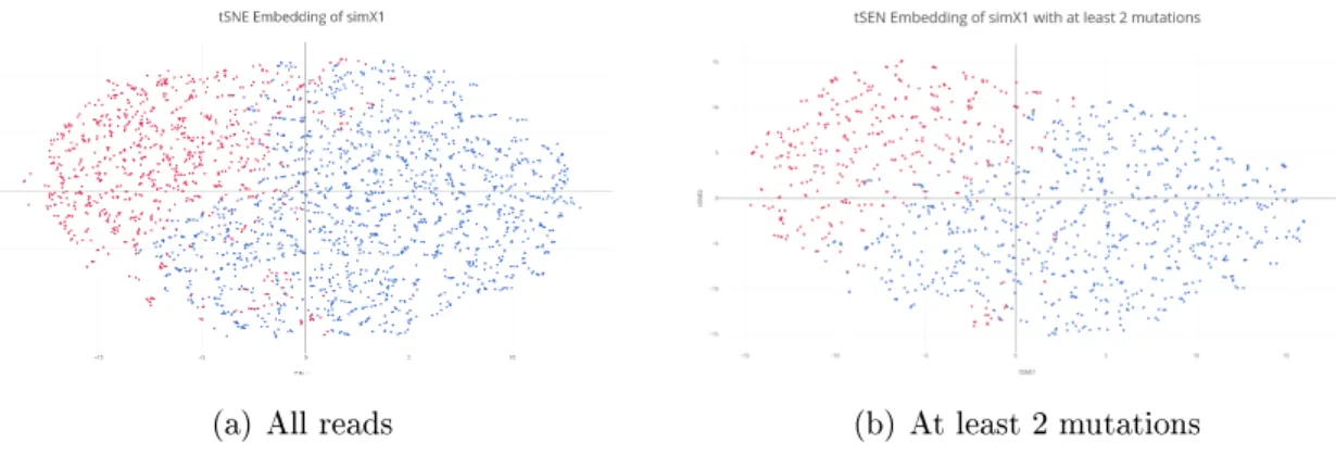
We define a minimum mutation per read cutoff, and select only reads matching this criteria. We evaluate this performance using a cutoff of 1 and of 2 (Figure 4-5, Table4.2). For values higher than 2, there were insufficient reads to obtain a reliable result.
(a) All reads (b) At least 2 mutations
Figure 4-5: Reads filtered for minimum mutation threshold.
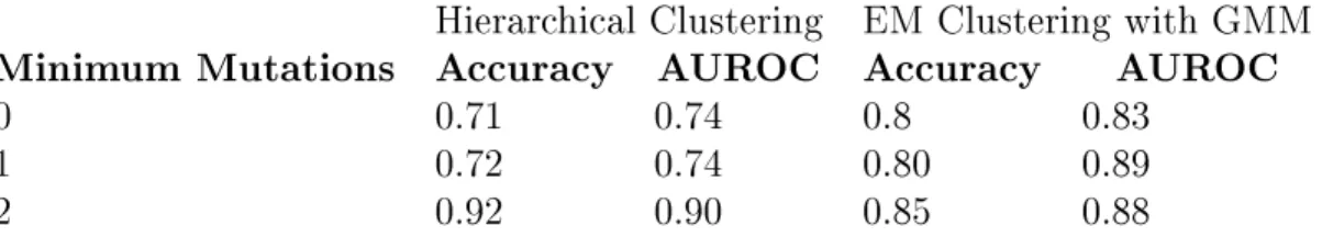
We observe a slightly improved performance for reads with at least one mutation and further improvement for reads with at least two mutations, an improvement which is most pronounced using hierarchical clustering. This makes sense, since reads with more mutations are likely to have stronger affinity for reads in their own cluster than reads with no mutations, which cannot be distinguished as coming from one structure or another. However, by
Hierarchical Clustering EM Clustering with GMM Minimum Mutations Accuracy AUROC Accuracy AUROC
0 0.71 0.74 0.8 0.83
1 0.72 0.74 0.80 0.89
2 0.92 0.90 0.85 0.88
Table 4.2: Accuracy of structure recovery for simX1 using mutation thresholding.
discarding reads in such a biased fashion, we may alter other aspects of our results by artificially increase the reactivity profile at certain positions, or altering the mixture proportions. For example,if one structure has fewer DMS accessible positions, more reads from this structure will be discarded, making its proportion appear smaller than in reality.
Nearest Neighbor Distances
Another possibility for improving the distance between reads from different clusters is to use an alternative distance metric, which emphasizes the distance between clusters more strongly. We propose an alternative metric based on the observation that reads from a given cluster are generated by the same structure. Therefore, if reads, 𝑟𝑖 and 𝑟𝑗 belong to the same
cluster, then 𝑟𝑖 should be quite close to the neighbors of 𝑟𝑗 as well.
Thus, we define a new dissimilarity function as follows (Figure 4-6).
𝛿𝑖𝑗 = 𝐷𝑖𝑗 + 𝛼1𝑖̸=𝑗(Σ𝑘∈𝐾𝑁 𝑁 (𝑗)𝐷𝑖𝑘+ Σ𝑘∈𝐾𝑁 𝑁 (𝑖)𝐷𝑗𝑘)
Figure 4-6: Alternative dissimilarity function incorporating nearest neighbor distances.
This metric satisfies the requirement for a dissimilarity function described above. We evaluate the results of this dissimilarity function, using 5 nearest neighbors, for various
values of 𝛼 on our simulated data (Table 4.3).
Hierarchical Clustering EM Clustering with GMM
𝛼 Accuracy AUROC Accuracy AUROC
0.0 0.71 0.74 0.8 0.83
0.2 0.78 0.83 0.83 0.87
0.5 0.78 0.82 0.84 0.87
2.0 0.71 0.76 0.63 0.67
20.0 0.60 0.58 0.68 0.67
Table 4.3: Accuracy of structure recovery for simX1 using nearest neighbor distances.
We observe very slightly improved classification accuracies for small values of 𝛼, peaking around 𝛼 = 0.5.
However, although more points are clustered together with other points from the same structure, we still do not observe significant separation between clusters, allowing us to visually determine the correct number of structures (Figure 4-7)
Figure 4-7: tSNE Embedding using Nearest Neighbor Distances
Since the performance of tSNE is not sufficient to observe distinct clusters in a simple RNA heterogeneous simulation, we explore the use of another embedding technique below.
4.3 Multidimensional Scaling
Multidimensional scaling [6] is another approach to low dimensional embedding which solves the following problem.
Given a distance matrix, 𝐷 ∈ R𝑛×𝑛, determine low dimensional points 𝑦
1, ..., 𝑦𝑛 ∈ R𝑞
𝑛 ∑︁ 𝑖=1 𝑛 ∑︁ 𝑗=1 (𝐷𝑖𝑗 − ‖𝑦𝑖− 𝑦𝑗‖)2
This approach is extended to dissimilarity matrices in non-metric MDS, in which the optimization problem has no closed solution but must be solved numerically. There are two major drawbacks to MDS. First, MDS is a numerical optimization technique, and, like t-SNE, it can fail to find the optimal solution by becoming stuck in local minima. Secondly, it is very slow due to the time-consuming numerical solution.
Results
We explore the use of MDS for clustering out simulated structures in simX1.
(a) MDS on All Reads (b) MDS using nearest neighbors for reads with at
least 2 mutations
Figure 4-8: Results of MDS Embedding on simX1.
We observe worse performance when using MDS compared to tSNE. This can be explained by that fact that tSNE focuses on preserving local structure, and less so on global distances. As such, tSNE has been found to yield superior performance in visualizing clusters.
4.3.1 Summary
Overall, we find that low dimensional representation methods like tSNE and MDS do not yield good results in separating alternative structures, and as such cannot provide an independent verification for our EM Clustering approach. If experimental advances lead to the possibility for increased signal on open bases or to modification on G and T bases as well, then the possibility of embedded clustering approaches may be revisited. However, in its current
form, the Expectation Maximization approach significantly outperforms low dimensional embedding.
Chapter 5
runDMC - A Web Platform for
DMS-MapSeq Analysis
In Chapter4, we evaluate independent methods for clustering RNA structure, and find that they are significantly outperformed by the EM clustering approach we previously developed at the Rouskin Lab. EM also uses data from chemical probing assays, such as DMS-MapSeq analysis, and provides a powerful tool for in vivo and in vitro detection of RNA structure and heterogeneity (Manuscript In Preparation). However, in order to analyze data from DMS probing and subsequent sequencing, there is a fairly detailed pipeline of computational steps that a biologist must undertake. This pipeline involved installing multiple dependencies, which means that it is difficult for scientists to immediately perform their analysis on any computing environment. Furthermore, the analysis is provided by a command-line tool, which is both cumbersome for large amounts of data analysis and deters experimentalists by its unintuitive interface.
In this chapter, we describe runDMC (run DMS Mutations Clustering), a web application which provides a simple, graphical user interface for immediate analysis of RNA probing data. We anticipate that this tool will simplify the process of RNA structure prediction and alternative structure detection, facilitating further scientific discovery.
5.1 User Analysis
In designing this web interface, we bear in mind the target audience and their specific characteristics. In order to understand the needs of the user, we perform several user interviews to identify the requirements of this user interface (UI). The current interface is implemented by a series of command line prompts on a Whitehead Server.
5.1.1 User Interviews
User 1:
User 1 is an experimental biologist who works on development in Drosophila melanogaster ovaries. Her expertise is primarily biological, and she describes herself as a novice when it comes to using computational tools. She describes her frustrations with the current work flow as follows: Sequencing samples typically have long names, which are difficult to type into a command line correctly. The commands are long and she often makes mistakes when typing sample names and parameters. This often leads to failed jobs which she has to rerun if she doesn’t notice a mistake. If she does realize that a mistake has occurred, she finds it annoying and time-consuming to retype the entire command. This failing is so serious that she often will not perform an analysis herself, but will wait for a more computationally experienced lab mate to perform thae analysis for her. Beyond the annoyances of the command line, she additionally does not like having to access the Whitehead server where the code is hosted, since access to this server requires repeated entry of her password and she cannot access her results when she is not connected to the Whitehead Institute network. The alternative of downloading the code from a GitHub repository and installing dependencies is even more intimidating to her.
Furthermore, she finds it very difficult to remember all commands and all the parameters needed. She keeps a file where she lists the commands and usually copy-pastes them into the terminal. However, this often leads to mistakes where she forgets to change a specific parameter, and then realizes she has performed analysis on the wrong region of interest after waiting several days for results.
of the results and connect them to samples. Although she employs a naming convention, she does not use it every time, and so she often forgets where the results of an analysis should be found, leading her to re-run the entire process or examine the wrong analysis results. Furthermore, it is time consuming for her to have to open each plot separately, and would like to be able to view them all quickly, without switching between folders in different locations. Finally, a text or graph output is not the most intuitive way for her to look at alternative structures, so she wishes it would be easier for her to look at her clustering results projected onto the RNA structure instead.
User 2:
User 2 is a graduate student studying virology at Harvard University. Although his expertise is primarily biological, he is familiar with computational tools, such as Python, and with command line interfaces.
He describes his frustrations with the current work-flow as follows. He does not like that after executing a command to perform analysis on a sample, he doesn’t know where in the stage of analysis he is. It becomes difficult for him to keep track of the jobs that are currently running and those that are completed, and he sometimes finds himself running the same analysis multiple times simultaneously.
When the analysis is complete, he becomes annoyed by having to navigate to many windows to open multiple samples, and by losing track of where the results are, and what sample they related to. Specifically, remembering the experimental conditions and regions being analyzed for a given result is difficult.
He often finds himself in the position where he has to share results with his other advisor or members of his team. He finds it cumbersome to aggregate all his results in a folder to zip this and share. He also finds it tiresome to have to explain each graph every time he sends the results to a less experienced user of the method. Indeed, he also sometimes finds it difficult to interpret the graphs produced and the sample quality checks, and would prefer having warnings displayed about the quality of his sample.
He also had concerns with running the code via a command line, finding it time-consuming and cumbersome to type long commands as well as determine data paths.
User 3:
User 3 is a principal investigator at the Whitehead Institute involved in RNA structure research. She is highly experienced in using command line tools, Python and other tools in computational analysis. However, she also has frustrations with the current command line interface. She has many samples to upload, so entering commands for each sample becomes time-consuming and repetitive, thus leading to many data entry errors.
In performing her analyses, she often has to fine-tune parameters to explore the performance on different samples. In the command line interface, it is difficult to keep track of the default parameters and very inflexible to change these parameters. Additionally, she finds it hard to remember which parameters were used in a given analysis.
The current pipeline consists of multiple stages, and if one stage fails, the entire analysis has to be re-run, or, if she simply wants to modify one aspect at a later stage in the analysis, she has to re-run the entire process. She would prefer to be able to have a more modular process, as well as view failed results which may be informative nonetheless.
She finds it difficult to compare the results of clustering, as it is not easy to see structural changes directly from a change in probability or observe which structures have similar mutation profiles. In order to do this, she uses another tool to independently generate structure illustrations. However, she often finds herself losing track of, and regenerating, the pictures from each clustering result, and keeping track of which structure corresponds to which sample becomes cumbersome.
She has multiple collaborators at various other institutions. They cannot access the internal server where the code is hosted, so they must download the code themselves and setup the environment required to run the analysis. They often are unable to install all the dependencies and set up the data paths correctly. This either leads to User 3 having to spend a significant amount of time showing them how to do this, or simply running their analyses for them. She finds it time-consuming to do this, and then explain their results to them, desiring a simpler view of results which would be easier for collaborators to understand.
5.1.2 User Classes
Based on our interviews, we define two primary user classes:
1. Power Users: This user class contains experimentalists who are also computationally experienced. They often have many samples to analyse, and prize being able to efficiently but accurately analyse their data. Some goals of this user class would be:
∙ Quickly input large numbers of samples for analysis
∙ Manage progress of multiple samples simultaneously and keep track of results ∙ Share results with collaborators in an easy to understand format.
∙ Easily view which regions in each alternative structure are accessible or occluded to look for functional differences.
2. Inexperienced Users: These users are often primarily experimental biologists who wish to have a simple, intuitive way of analyzing data. They do not want to deal with program dependencies, setting up computing environments or navigating command line interfaces. Some goals of this user class would be:
∙ Upload a sample and check on its progress in analysis
∙ Decide whether results can be trusted, given the experimental data
∙ View results in the context of resulting biological interpretation - what is the bottom line of the structural change.
∙ Easily view which regions in each alternative structure are accessible or occluded to look for functional differences.
5.1.3 Interface Goals
Based on the feedback received from user interviews, we describe the interface goals of runDMC as follows.
1. Simple. The runDMC user interface must above all provide an interface which is simple and usable for a non-technical user. This must be reflected in both the data upload, requiring a minimal amount of user parameter tuning, as well as in the results being displayed.
2. Intuitive and Detailed Results. The results of runDMC must be presented in such a way that the details of the analysis are explicit so that experimental failures or anomalies can be quickly detected, allowing experimentalists to determine whether the computational analysis can be trusted. Furthermore, the results should be presented in such a way that they intuitively provide insight into the biology, rather than some abstracted understanding.
3. Flexible. runDMC must provide a flexible interface for both inexperienced users, who want a streamlined, simple experience, as well as power users, who will often want to experiment many settings of parameters and have fine-grain control over the analysis. 4. Quick. Power users describe the need to analyse large numbers of samples, requiring an interface which allows a very fast upload so that they can process all their samples quickly.
5. Organized. Users must be able to collect all the details of an analysis together in an organized fashion, so that parameters and inputs relevant to the results are stored alongside the results.
With these goals in mind, we present the implemetation details and design of runDMC in the following section.
5.2 Implementation
5.2.1 Back-end Infrastructure
The back-end component of runDMC does the heavy lifting of the analysis. It is responsible for the various data input and validation tasks, the implementation of DMS data analysis, the EM clustering algorithm, and serving data for visualization of results to the front-end component.
The back-end server for runDMC is implemented using Django, a Python based framework. Django follows the Model-View-Template architectural pattern, and provides a highly adaptable template system and reusable components, which are key in providing a framework for rapid iterations and development. Celery is used to provide a task queue to distribute work across threads. Using this distributed system is key in processing vast quotas of messages, allowing us to handle large files of sequencing data. Celery employs multiple workers and brokers, giving way to high availability and horizontal scaling.We use Redis as a broker to send and receive messages between Celery and our Django framework.
Database capabilities are enabled by an SQLite server. The database design is as shown in Figure5-1. The running Django instance is served by Apache, a popular free and open-source webserver, and is hosted on a server at the Whitehead Institute for Biomedical Research.
In addition to its strengths in simplifying web development, Django, as a Python based framework, integrated well with the code for analysis. All scripts used were developed using Python.
For RNA structure prediction, we use the RNAStructure package developed by the Matthews Lab at the University of Rochester Medical Center [11]. Specifically, we use the Fold tool which minimizes the free energy of the folded structure, and accepts DMS data constraints to inform these predictions.
Figure 5-1: Database Schema for runDMC
5.2.2 Front-end Infrastructure
The front-end component which provides the user interface is implemented using HTML, CSS and JavaScript. We use Bootstrap, front-end component library, to create a uniform aesthetic and facilitate quick design prototyping. Data visualizations are done using plot.ly [14], a D3.js (Data-Driven Documents) based plotting library to create interactive and informative visualizations.
5.3 Design
In this section, we present the design of the runDMC user interface, which reflects the interface goals determined from the user interviews.
Login
We present a simple interface for logging in by either creating an account or using the Google+ API to facilitate login using Gmail. This provides a quick way of using runDMC and allows for easier management and organization of uploaded samples.
Figure 5-2: The user can view further details about a job
By implementing account management on runDMC, we allow all samples to be associated with a specific user. This enables us to collect all their results in an organized manner for subsequent viewing.
Sample Uploads
Upon login, the user is immediately redirected to the upload page (Figure 5-3). This is useful for both inexperienced and power users, since they can quickly upload samples without wasting time or getting confused by having to navigate to the data upload page. The upload
page provides a simple interface, displaying only required fields initially. Default values are shown as placeholders to provide intuition for reasonable values, and help text is provided for each entry field using the help icons positioned adjacent to the respective input fields.
Figure 5-3: Interface provides streamlined graphical interface for upload and parameter selection
For power users who wish to have more control over details, a section on advanced parameters is available via a drop-down menu, from which they can modify further parameters, as well as view the defaults used by the algorithm (Figure 5-4).
Figure 5-4: Advanced parameters are available for modification by power users, but otherwise abstracted away
well as detailed error messages so that the user does not submit a job, realize it has failed and then be forced to re-submit the job later on without first addressing the source of the error.
Following the submission of a job, the user is re-directed to a success page (Figure 5-6), confirming the job’s submission and providing a quick link for further sample upload. This allows power users who have many samples to upload to establish a logical and simple flow for continuously uploading samples, reducing the time spent to navigate back to the uploads page and begin the process again.
When a user is logged in, they can see their user name in the upper right hand corner (Figure 5-6). This is a drop-down menu, indicated by the arrow affordance, which user can click on. The menu displayed allows them to either logout of runDMC or navigate to their submitted jobs.
Figure 5-5: Error messages are provided to highlight mistakes in data entry.
User Jobs
In order to facilitate easier management of samples and analysis progress, we create a view of the uploaded samples, date of upload as well as status (Figure5-7).The status may be either ’SUCCESS’, ’Failed’ or ’In Progress’, indicating whether the analysis is complete, resulted in an error or is still running.
The sample ID allows users to contact the administrator about specific questions about a sample, and clicking on the sample ID, the user can view all the details about that sample. This becomes useful when examining results after some time has passed, so that keeping track of experimental details becomes easier. We additionally provide a small ’Details’ section where the user can jot down notes relating to the sample for reference at a later date (Figure 5-8).
Upon completion of a job, the user receives an email with a link to the results if successful, or an error log if the job fails. However, keeping track of the link via email is cumbersome and begets disorganization. Therefore, if a job is successful, they can access the results by clicking on the success button next to the sample ID. During interviews, users expressed a desire to be able to view the progress of their jobs, as well as to view partial results in the case of failure. As such, the Results page can be accessed before a job is terminated, and includes all the results generated up to that point. Combined with the log file emailed to the user in case of a failure, this allows users to potentially troubleshoot issues with their experimental data or upload parameters.
Additionally, users can use the intuitive red trash icon to delete any analyses that they no longer wish to keep. Following a confirmation dialog for safety, these analyses are removed from the model database and cannot be accessed again.
Figure 5-8: Details of a sample are provided for easier sample management, along with the facility for free form notes.
Results
The results are displayed in the form of a report, with a drop down menu to navigate through the different sections of results, described below.
1. Results Downloads 2. Sample Statistics 3. Population Average 4. Clustering Results
Figure 5-9: Results are presented in a report format to easily view all aspects of the analysis
On the Results page, users can choose to download zipped files of the bitvector created, the clustering results or all the files generate by the analysis (Figure 5-10). They can then access the results off-line and perform further analyses.
Figure 5-10: Directory of all results generated by the analysis.
We display and further discuss the actual results displayed later on the page in further detail in the following section.
5.4 Data Analysis and Results
In this section, we discuss the required inputs as well as the results generated by runDMC, and describe the visualizations corresponding to these results.
5.4.1 Inputs
The user first follows the experimental protocol for DMS MaPseq, outlined in [16], for their sample and region of interest. The user inputs aligned reads, in the form of a SAM or BAM [8] file. This is the output of an alignment, often using bowtie2 [7] which maps sequenced reads to a reference sequence. This allows us to identify whether a mutation relative to the reference has occurred. Additionally, the user must input several parameters, identifying a region of interest and analyzing that region. In order to identify this region, the user must specify a reference gene, as well as genomic coordinates on this reference. Alternatively, they may specify the forward primer and reverse primer used in their experiment, and the region of interest will be inferred.
In order to have a simple and intuitive interface, we provide defaults and placeholders for all inputs, and only require the minimal set of inputs. Once these inputs have been validated, we submit the task to the Celery queue and generate the results.
5.4.2 Sample Statistics
In order to know whether the result of the computational analysis can be trusted, the user must first be convinced of the quality of the sample. In order to provide information for the user to make this decision, we first display a plot showing the coverage achieved by their sample, as show in Figure5-11.
This plot shows the coverage of all the aligned reads along the reference of interest. This allows the user to determine whether the experiment was successful in:
1. Using primers that allow selection of the correct region of interest
2. Having sufficient coverage in the region of interest, allowing them to either modify PCR cycles or sequencing depth.
3. Having read fragments being of the expected length, and not overly fragmented due to excessively high DMS concentrations
Figure 5-11: The number of data points used in the analysis is displayed, and warnings provided to ensure sufficient sample size.
If the region coverage is not as expected, the user can know that there was an experimental error in the sample, and so they should not trust the results of the analysis.
To improve the intuition for interpreting results, we provide errors, warnings and success messages for critical aspects of the analysis. For example, if coverage of the region of interest is too low, then we display either an error or warning, depending on the severity of the problem. Otherwise, the user receives a message signalling they the results of the analysis can be trusted. These messages are displayed using different color-coded icons - red, orange or green - as affordances to indicate the severity of the issue.
Mutations per Nucleotide
We compute and display the number of mutations/mismatches which occur on each nucleotide as shown in Figure 5-12. Theoretically, DMS should only modify open A/C nucleotides. However, in practice this is not always true. In order to estimate the false positive rate, we compute the number of mutations occurring at each base. Mutations occurring on G/T nucleotides can provide insight into the noise of the sample, allowing the user to determine whether the experiment was likely to have been successful. If the false positive rate is higher than 10%, the user is warned about this issue.
Figure 5-12: The number of mutations on off-target bases informs the false positive rate.
Mutations per Read
We compute the distribution of the number of mutations occurring on each read, as shown in Figure 5-13. This allows the user to determine whether there are any anomalous reads, containing significantly higher number of mutations than would be expected. DMS modification is a probabilistic process, modifying open bases with a low probability. Thus, we do not expect many reads to have large numbers of mismatched positions. Such reads can indicate poor alignments, sequencing error, or other experimental issues. The number of mutations
per read depends on the length of the sequence as well as the structure, since longer sequences will naturally have more positions capable of being modified but more structured regions have less bases accessible to DMS. However, the user can inspect this graph to ensure there are few outlier reads with too many mutations.
Figure 5-13: The number of mutations per reads can reveal outliers.
RT Enzyme Inserted Bases
For every mismatched position, we count the number of times each possible base was inserted by the RT enzyme. Theoretically, we expect a random base to be inserted on every DMS modified position.
This figure (Figure 5-14) allows the user to examine this assumption, as well as identify endogenously modified bases, since they will have primarily one inserted base at that position. We can also identify biases in the RT enzyme for different bases. For example, in the sequence above and generally, we observer a strong preference for inserting ’T’ nucleotides.
Figure 5-14: We generate interactive plots showing sample statistics to help assess experimental success.
5.4.3 Population Average
Bitvectors
The first aspect of DMS analysis involves the creation of a bitvector, which allows us to identify positions where DMS mutations occur. We consider the size of the region of interest, specified by the reference gene and the genomic coordinates within this gene. We then collect all reads which overlap with the region of interest and calculate the positions where mismatches occurred (most likely) due to DMS modifications. Each read produces a bitvector - a string the length of the region of interest, containing a 0 where the read matches the reference, otherwise containing the nucleotide which was inserted in place of the reference nucleotide or a D if a deletion occurred at that position. If the read does not contain information corresponding to that position, then we include a ’.’ at that position to indicate the lack of coverage. Poor quality positions, based on the quality reported by the sequencer, are indicated by ’?’, and are not used later in analysis. Our prior on a mutated position is much lower than our prior on a position matching the reference sequence, so we report bases as low quality if they match the reference and have an accuracy lower than 50%, or they are a mismatch and have an accuracy lower than 99%.