Factor analytical modeling of C₂?C₇ hydrocarbon sources at an urban background site in Zurich (Switzerland): changes between 1993?1994 and 2005?2006

HAL Id: hal-00303256

https://hal.archives-ouvertes.fr/hal-00303256

HAL is a multi-disciplinary open access

archive for the deposit and dissemination of sci-entific research documents, whether they are pub-lished or not. The documents may come from teaching and research institutions in France or abroad, or from public or private research centers.

L’archive ouverte pluridisciplinaire HAL, est destinée au dépôt et à la diffusion de documents scientifiques de niveau recherche, publiés ou non, émanant des établissements d’enseignement et de recherche français ou étrangers, des laboratoires publics ou privés.

Factor analytical modeling of C2?C7 hydrocarbon

sources at an urban background site in Zurich

(Switzerland): changes between 1993?1994 and

2005?2006

V. A. Lanz, B. Buchmann, C. Hueglin, R. Locher, S. Reimann, J. Staehelin

To cite this version:

V. A. Lanz, B. Buchmann, C. Hueglin, R. Locher, S. Reimann, et al.. Factor analytical modeling of C2?C7 hydrocarbon sources at an urban background site in Zurich (Switzerland): changes between 1993?1994 and 2005?2006. Atmospheric Chemistry and Physics Discussions, European Geosciences Union, 2008, 8 (1), pp.907-955. �hal-00303256�

ACPD

Full Screen / Esc

Printer-friendly Version Interactive Discussion

EGU Atmos. Chem. Phys. Discuss., 8, 907–955, 2008

www.atmos-chem-phys-discuss.net/8/907/2008/ © Author(s) 2008. This work is licensed

under a Creative Commons License.

Atmospheric Chemistry and Physics Discussions

Factor analytical modeling of C

₂

–C

₇

hydrocarbon sources at an urban

background site in Zurich (Switzerland):

changes between 1993–1994 and

2005–2006

V. A. Lanz1, B. Buchmann1, C. Hueglin1, R. Locher2, S. Reimann1, and J. Staehelin3

1

Empa, Swiss Federal Laboratories for Materials Testing and Research, Laboratory for Air Pollution and Environmental Technology, 8600 Duebendorf, Switzerland

2

ZHAW, School of Engineering, Institute of Data Analysis and Process Design IDP, 8401 Winterthur, Switzerland

3

Institute for Atmospheric and Climate Science, ETH Zurich, 8092 Zurich, Switzerland Received: 28 November 2007 – Accepted: 9 December 2007 – Published: 18 January 2008 Correspondence to: V. A. Lanz (valentin.lanz@empa.ch)

ACPD

Full Screen / Esc

Printer-friendly Version Interactive Discussion

EGU

Abstract

Hourly measurements of 13 volatile hydrocarbons (C2–C7) were performed at an urban

background site in Zurich (Switzerland) in the years 1993–1994 and again in 2005– 2006. Changes in hydrocarbon profiles and source strengths were recovered by pos-itive matrix factorization (PMF). Eight and six factors could be related to hydrocarbon

5

sources in 1993–1994 and in 2005–2006, respectively. The modeled source profiles were verified by hydrocarbon profiles reported in the literature. The source strengths were validated by independent measurements, such as inorganic trace gases (NOx,

CO, SO2), methane (CH4), oxidized hydrocarbons (OVOCs) and meteorological data

(temperature, wind speed etc.). Our analysis suggests that the contribution of most

10

hydrocarbon sources (i.e. road traffic, solvents use, and wood burning) decreased by a factor of about two to three between the early 1990s and 2005–2006. On the other hand, hydrocarbon losses from natural gas leakage remained at relatively constant (−20%) concentration levels. The estimated emission trends are in line with the results from different top-down approaches reported for other European cities. Their

discrep-15

ancies to national emission inventories are discussed.

1 Introduction

Air pollutants can have adverse impacts on human health, most notably on the respira-tory system and circulation (Nel, 2005), acidify and eutrophicate ecosystems (Matson et al., 2002), diminish agricultural yields, corrode materials and buildings (Primerano et

20

al., 2000), and decrease atmospheric visibility (Watson, 2002). Organic pollutants are very complex regarding their composition, properties and chemical processes. Organic gases and particles can both be directly emitted into the atmosphere, e.g. by fossil fuel combustion, or secondarily formed and decomposed there by chemical reactions and/or gas-to-particle conversions (Fuzzi et al., 2006). Volatile organic compounds

25

ACPD

Full Screen / Esc

Printer-friendly Version Interactive Discussion

EGU e.g. benzene (WHO, 1993), or relevant greenhouse gases, e.g. methane (Forster et

al., 2007), all VOCs are oxidized in the atmosphere and most are thereby involved in the formation of secondary pollutants, such as ozone (O3), and secondary organic

aerosol (SOA). Ambient VOC measurements got special attention since the 1950s due to summer smog phenomena, first and foremost due to high O3levels in the Los Ange-5

les basin (Eggertsen and Nelsen, 1958). The identification and quantification of VOC sources is therefore a necessary step to mitigate air pollution.

Receptor models were developed to attribute measured ambient air pollutants to their emission sources. Depending on the degree of prior knowledge of the sources, a chemical mass balance (CMB; composition of the emission sources is known), a

mul-10

tivariate receptor model (no a priori knowledge) or a hybrid model in between these extreme cases is most appropriate (Christensen et al., 2006). The first multivariate source apportionment studies were about the elemental composition of particulate mat-ter (e.g. Blifford and Meeker, 1967). In contrast to organic species, they do not react in ambient air. Given that their sources emit those elements in constant proportions over

15

time, the calculated receptor profiles can directly be related to sources. Receptor mod-els have also been applied to speciated organic data since detailed information about the chemical composition of volatile and semi-volatile organic compounds is available, provided e.g. by high-resolution gas-chromatography (Schauer et al., 1996) or aerosol mass spectrometry (Lanz et al., 2007). However, the fundamental assumption of

non-20

reactivity or mass conservation (Hopke, 2003) can be violated and the calculated fac-tors may not always be directly related to emission profiles but have to be interpreted as aged profiles (depending on the selected species and measurement location). There-fore, a flexible model such as positive matrix factorization (PMF; Paatero and Tapper, 1994) is favorable to model VOC concentration matrices. Furthermore, PMF modeling

25

allows for any changes (e.g. local differences) in the nature of the VOC sources. The PMF2 program (Paatero, 1997) uses a stable algorithm to estimate source strengths and profiles from multivariate data sets (bilinear receptor-model). Miller et al. (2002) concluded for simulated data that PMF was superior in recovering VOC source profiles

ACPD

Full Screen / Esc

Printer-friendly Version Interactive Discussion

EGU compared to other receptor models based on standard CMB (Winchester and Nifong,

1971), principal component analysis (Blifford and Meeker, 1967) or UNMIX, a multi-variate receptor model developed by Henry (2003). Also Jorquera and Rappengl ¨uck (2004) found PMF resolved VOC profiles more reliable than profiles resolved by UN-MIX, while Anderson et al. (2002) found the results of the two models to be in good

5

agreement. Further evidence that bilinear unmixing by PMF2 can be used to model VOC data was provided for the Texas area (Buzcu and Frazier, 2006), where for cer-tain emission situations (e.g. wind directional dependencies of point sources etc.) an enhanced PMF was favorable (Zhao et al., 2004).

Due to the environmental problems mentioned above, abatement strategies have

10

been developed and implemented for the reduction of VOC emissions. In fact, the sum of non-methane VOCs at an urban background location in Zurich (Switzerland), as an example, decreased by -50% from the late 1980s to the early 1990s and again by -30% from the early 1990s to today (Fig. 1). For 1993–1994, about 20 volatile hydrocarbon species were determined at Zurich-Kaserne by hourly resolved gas-chromatography

15

(GC-FID). For 2005—2006, more than 20 hydrocarbons were measured again at the same site (13 of them were measured during both periods and are summarized in Ta-ble 1 and Fig. 2). By PMF modeling of hydrocarbon observations in 1993–1994 and in 2005–2006 we describe the underlying factors of each data set. The factors recovered by multivariate PMF modeling are related to hydrocarbon source profiles and source

20

strengths. This attribution needs to be verified by means of collocated measurements (inorganic trace gases, oxidized hydrocarbons, meteorology), by time series analysis of the source strengths as well as by published VOC profiles and emission factors from the literature. The decrease in ambient VOC concentrations between the early 1990s and today (2005–2006) is explained by comparing the factor analytical results for both

25

ACPD

Full Screen / Esc

Printer-friendly Version Interactive Discussion EGU 2 Methods 2.1 Measurements 2.1.1 Hydrocarbon measurements

The measurements at Zurich-Kaserne (410 m a.s.l.) represent an urban background site in Zurich, Switzerland. It is located at a public backyard near the city center. The

5

earlier VOC measurements in 1993–1994 were presented by Staehelin et al. (2001). The time spans in this study included 4 June 1993 to 6 October 1994 and 4 June 2005 to 6 October 2006.

18 hydrocarbons were measured quasi-continuously in Zurich between 1993 and 1994: first, ambient air was passed through a Nafion Dryer to minimize its water

con-10

tent and was then extracted from hydrocarbons using an adsorption-desorption unit (VOC Air Analyzer, Chrompack) equipped with a multi-stage adsorption tube at −25◦C. The flow of air through the trap was 10 ml min−1 and the trapping time was 30 min, yielding a total volume of 300 ml of sampled air. Then the trap was heated to 250◦C for transferring the VOCs to a cryo-focussing trap (Poraplot Q), held at −100◦C.

Fi-15

nally, concentrated VOCs were passed onto the analytical PLOT column (Al2O3/KCl,

50 m×0.53 mm, Chrompack) by heating to 125◦C. The analysis was performed by gas chromatography-flame ionization detection (GC-FID, Chrompack). Calibration was per-formed regularly by diluting a commercial standard with zero air to the lower ppb (parts per billion by volume) range.

20

22 hydrocarbons were measured quasi-continuously in 2005–2006: First, ambient air was passed through a Nafion Dryer to minimize its water content and was then extracted from hydrocarbons using an adsorption-desorption unit (Perkin-Elmer, TD), equipped with a multi-stage microtrap held at −30◦C by means of a Peltier element. The flow of air through the trap was 20 ml min−1 and the trapping time was 15 min,

25

yielding a total volume of 300 ml of sampled air. After flushing with helium to reduce the water vapor content the trap was rapidly heated to 260◦C for desorption of the

hy-ACPD

Full Screen / Esc

Printer-friendly Version Interactive Discussion

EGU drocarbons onto the analytical PLOT column (Al₂O₃/KCl, 50 m×0.53 mm, Varian). The

analysis was performed by gas chromatography-flame ionization detection (GC-FID, Agilent 6890). Calibrations were performed regularly using a standard which contains the analyzed hydrocarbons in the lower ppb range (National Physical Laboratory, UK). 13 hydrocarbon species were measured in both data sets (summarized in Table 1

5

and Fig. 2) and used for the statistical analysis. Ethane measurements were not quan-titatively determined in 1993–1994, but we can assume (based on comparisons with quantitatively measured compounds) that the reported signals are proportional to the real concentrations and therefore do not influence the PMF analysis.

2.1.2 Ancillary data

10

About 20 different, hourly resolved OVOCs are available at Zurich-Kaserne for cam-paigns in summer 2005 and winter 2005/2006. The measurements were performed by GC-MS (gas chromatograph with mass spectrometer) and summarized in Legreid et al. (2007a). Inorganic trace gases (NO_x, CO, SO₂), meteorological parameters (tem-perature, wind speed etc.), methane (CH4), and t-NMVOC were measured by standard 15

methods (Empa, 2006). Measurements of t-NMVOCs are performed continuously by a flame ionization detector (FID) (APHA 360, Horiba). For separation between CH₄ and t-NMVOCs the air sample is divided into two parts. One part is directly introduced into the FID, while the second part is lead through a catalytic converter to remove the NMVOCs. The outcome of both lines is measured alternately and the t-NMVOC

20

ACPD

Full Screen / Esc

Printer-friendly Version Interactive Discussion

EGU 2.2 Data analysis and preparation

2.2.1 Unmixing multivariate observations

Linear mixing of observable quantities is the basis to all receptor models and can be represented by the following equation (Henry, 1984):

x

i=giF+ei, (1)

5

where x_i represents the i-th multivariate observation (vector of m variables) and is ap-proximated by linear combinations of the loadings or source profiles (F) and scores or source strengths (g_i) up to an error vector e_i. Chemical mass balance models were designed for estimation of source strengths, g_i (a p-dimensional vector), for given nu-merical values of F, representing a p×m-matrix of the source profiles, and a specified

10

number of assumed factors or sources p. Multivariate receptor models, on the other hand, are most useful when very little or no prior knowledge about the sources is as-sumed. In such a case, both gi and F have to be estimated, and p has to be determined

by exploratory means. Paatero and Tapper (1994) have proposed to solve Eq. (1) by a least-square algorithm minimizing the uncertainty weighted error (“scaled residuals”):

15

eij/si j=(xij−gi pfpj)/si j (2)

The associated software PMF2 (Paatero, 1997) minimizes the sum of (e_ij/s_ij)2(called Q) for all samples i=1. . .n and all variables j=1. . .m. In practice, an enhanced Q is to be minimized, accounting e.g. for penalty terms that ensure a non-negative solution to Eq. (1). This approach implicitly assumes that uncertainties, s_ij, for each element

20

of the multivariate data set,x_ij, are known. For VOC species, an ad hoc uncertainty calculation has been suggested by Anttila et al. (1995) and was used in many studies (e.g. Fujita et al., 2003, and Hell ´en et al., 2006):

s2_ij=4 (DL)2j+(CV )

2

j x

2

ACPD

Full Screen / Esc

Printer-friendly Version Interactive Discussion

EGU where DL represents the detection limit (as an absolute concentration value) and the

coefficient of variation, CV, accounts for the relative measurement error determined by calibration of the instruments. The DLs equal five times the baseline noise of the species’ chromatograms, whereas the CV s are the relative standard deviations of six repeated measurements of a real-air standard in the range of ambient concentrations.

5

Following this method, both DL and CV are species-specific and given in Table 1 for the present hydrocarbon data sets.

2.2.2 Model specifications and reactivity

For the presented results, the PMF2 program was run with default settings (robust mode, central rotation induced by fpeak =0, outlier thresholds for the scaled residuals

10

of −4 and 4), but the error model (E M=−14) was adjusted for ambient data. A relatively high modeling uncertainty of 10% was assumed as the atmospheric lifetimes (due to reactions with OH radicals) of the considered VOC species vary widely: from 0.6 days (propene) to 55 days (ethane). We assumed that the VOC variability at the urban site Zurich-Kaserne is generally driven by source activities rather than by ageing of the

15

compounds; VOC transport time from source to receptor was assumed to be less than 0.5 day on average, which is smaller than the lifetime of propene, the most reactive compound analyzed in the study. Furthermore, we have imposed an aged VOC profile – averaged during a high pressure episode at a remote location (Rigi-Seebodenalp, 1030 m a.s.l., about 40 km Southeast of Zurich) – on the Zurich-Kaserne data by using

20

a hybrid receptor model in between CMB and PMF following the approach described in Lanz et al. (2008). The resulting source contributions indicated that down-mixing of aged air masses is not a relevant process that influences VOC variability at this location.

ACPD

Full Screen / Esc

Printer-friendly Version Interactive Discussion

EGU 2.2.3 Missing values

In 1993–1994, missing ethane and ethyne concentrations had to be imputed for n=3450 and n=1500 samples, respectively (∼ 5% of data matrix). Row-wise dele-tion of those missing values would have caused a loss of 50% of the data. We in-stead have used the k-nearest neighbor (knn) method to estimate those missing values

5

(function knn of the EMV package in R, The R Foundation for Statistical Computing; www.r-project.org). Additional VOCs were considered for the nearest-neighbor calcu-lations (e.g. 2,2,4-trimethylpentane, 2-methylpropene, and heptane). Advantages of data imputation by multivariate nearest neighbor methods in the field of atmospheric research were evaluated by Junninen et al. (2004): they are particularly important for

10

practical applications as they are fast, perform well, and do not generate new values in the data. We calculated (by repetitively and randomly assigning missing values to known values) that the relative uncertainty of this imputational method is about 48% (1σ) for ethane and about 32% (1σ) for ethyne. Calculating the uncertainty matrix, the imputed concentration values of ethane and ethyne were multiplied by 0.96 (2σ) and

15

0.64 (2σ), respectively, and the square of this product was added to the error as stated by Eq. (3):

s_ij2=4(DL)2_j+(CV )2_jx_{i j}2+(2σxi j)2, xijimputed (4)

In summary, this additional term down-weights the imputed values by a factor of about 10. Even though the imputed values have a minor weight in the minimization algorithm

20

of PMF2, factors characterized by ethane or ethyne for the 1993–1994 data should nevertheless be carefully interpreted.

2.2.4 Outliers in the data (local contamination)

Propane peaks up to 400 ppb (2005–2006) and 200 ppb (1993–1994) could be ob-served and were most probably caused by local barbecue events. We have defined

25

ACPD

Full Screen / Esc

Printer-friendly Version Interactive Discussion

EGU About 70 samples were identified and excluded from both data sets in order to not

distort the factor analysis. A detailed inspection of the deleted samples revealed that these propane peaks mostly occurred on/before weekends and holidays during the summery season, supporting the hypothesis of local barbecue emissions in the public backyard surrounding the measurement site. In 2005–2006, a threshold of σ rather

5

than 2σ was needed to identify a similar fraction (∼1%) of contamination type outliers. 2.2.5 Robustness of the PMF solution

In order to test the robustness of the presented results, we made additional PMF runs with 21 hydrocarbons available since 2005 (the sum of butenes was deleted column-wise from the data matrix due to its abundant missing values). Isoprene and

1,3-10

butadiene were found to determine two additional factors almost alone due to their distinct temporal behavior in ambient air: both VOCs are rapidly removed by radical reactions. Their atmospheric lifetime is in the order of minutes to hours and these compounds therefore change the variability structure of the data matrix. However, isoprene and 1,3-butadiene accounted for less than 1% of the total concentration (in

15

ppb) given by the 22 hydrocarbons retrieved since 2005 at Zurich-Kaserne. Therefore, the exclusion of these latter compounds does not influence the representativeness, but yields robust results. On the other side, aromatic C₈hydrocarbons, which were highly correlated (R>0.97), summed up to considerable concentrations, but did not alter the variability pattern in the data (see Sect. 3.5.1).

20

3 Results and discussion

3.1 Determination of the number of factors (p)

The determination of the number of factors p is a critical step for receptor-based source apportionment methods, especially for multivariate models, where very little

ACPD

Full Screen / Esc

Printer-friendly Version Interactive Discussion

EGU prior knowledge about the sources is assumed. Mathematically perfect matrix

decom-positions into scores and loadings do not guarantee that the solutions are physically meaningful and can be interpreted. Here, we followed the philosophy that an appropri-ate number of factors has to be determined by means of interpretability and physical meaningfulness as already proposed earlier (e.g. by Li et al., 2004; Buset et al., 2006;

5

Lanz et al., 2007 and 2008). Mathematical diagnostics are however indispensable to corroborate the chosen solution and to describe the mathematical aspect of its ex-planatory power.

For the recently (2005–2006) measured VOCs, up to 6 factors can be interpreted. A detailed discussion of the interpretation of the 6-factorial solution can be found in

10

Sects. 3.3 and 3.4. Choosing 5 and less factors coerces two profiles (attributed to “sol-vent use” and “gasoline evaporation”; see Sect. 3.3). On the other hand, by choosing 7 factors and more, a factor splits from the “gasoline evaporation” factor (the sum of two split contributions is very similar to 6-factorial gasoline source, R=0.97). We therefore consider the 6-factorial solution for further analyses of the VOC sources in 2005–2006.

15

For the earlier VOC series (1993–1994), we have most confidence in the 8-factorial so-lution: when assuming 8 factors, for each of the 6 factors found in 2005–2006 a similar factor is found as in the earlier measurements (plus a toluene source and an additional, combustion-related source). This can not be observed for solutions where more than 8 factors or less than 8 factors were imposed.

20

The data sets from 1993–1994 and 2005–2006 had to be described by a different number of factors each (eight and six, respectively) in order to account for the different emission situations: two factors were absent in the 2005–2006 data, which can be explained by policy regulations (see Sects. 3.4 and 4).

3.2 Mathematical diagnostics

25

More than 93% and 96% of the variability of the VOC species could be explained on average by the 6-factorial model (2005–2006) and the 8-factorial model (1993–1994), respectively (see concept of explained variance; Paatero, 2007). Using the proposed

ACPD

Full Screen / Esc

Printer-friendly Version Interactive Discussion

EGU model we can further explain on average 97% and 99% of the VOC concentrations

(in ppb) measured in 2005–2006 and 1993–1994, respectively. For both models, less than 1% of all data points (about 100 000 for both data sets) exceeded the model outlier thresholds for the scaled residuals and were down-weighted (Sect. 2.2). The Q-value, the total sum of scaled residuals, equals 11 275 in the robust-mode for the 1993–1994

5

data (n=7606, p=8). For 2005–2006 (n=8912, p=6), this value is 70 018. Thus, for both data sets the calculated Q is in the order of the expected Q, estimated by mn-p(m+n) as a rule of thumb. The scaled residuals for each species and both data sets are approximately normally distributed N(0,σ_j).

3.3 Hydrocarbon profiles and first-guess attribution to emission sources

10

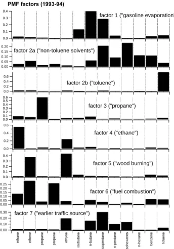
In this section, the factor profiles as retrieved by PMF for 1993–1994 and 2005–2006 are summarized (Table 2) and discussed. We introduce a tentative attribution of PMF factors to emission sources based on a priori knowledge such as published source profiles. The factors underlying the recent measurements (Fig. 3) and the ones ex-plaining the earlier VOC data (Fig. 4) are compared with each other, with reference

15

profiles found in the literature, and with profiles reported in Staehelin et al. (2001). The factors for the recent data (2005–2006) were sorted on the basis of explained variance (Paatero, 2007). The factors calculated for the earlier data (1993–1994) were rearranged according to the order of the factors retrieved from the recent data (2005– 2006).

20

3.3.1 Profiles for the years 2005-2006

The variability described by factor 1 is dominated by contributions of (iso-)pentane, isohexanes, (iso-)butane and it includes toluene and benzene (Fig. 3). This feature is shared by gasoline evaporation as well as gasoline combustion as can be de-duced from the VOC profiles reported in Theloke and Friedrich (2007). In fact, the

25

ACPD

Full Screen / Esc

Printer-friendly Version Interactive Discussion

EGU therein: two-stroke engine, urban mode, warm (R=0.94, n=13) and cold start phase

(R=0.94, n=13) as well as with gasoline evaporation (R=0.97, n=7). Thus, based on its fingerprint alone factor 1 could be related to gasoline combustion and/or gasoline evaporation. A more specific interpretation of this first factor is given in Sect. 3.4.1.

In factor 2, prominent toluene, isohexane and isopentane contributions can be

ob-5

served and most of the toluene (61%), isohexanes (52%), hexane (48%), pentane (40%) and isopentane (40%) variability is explained by the second factor. This factor is only weakly influenced by the variability of combustion related C₂–C₄ hydrocarbons (<10%). We therefore attribute this factor to solvent use.

Given the hydrocarbon fingerprint only, factor 3 (propane and butane) and factor 4

10

(ethane) could be related to many different sources (natural gas distribution and/or combustion, gas grill emissions, petrol gas vehicles etc.). Because benzene and toluene do not influence this third factor, we tend to attribute these factors to gas leak-age or a “clean” combustion source. Furthermore, factor 4 is dominated by ethane and potentially could also represent an aged background profile; ethane is the longest lived

15

species considered in this study. In the Northern Hemisphere, ethane and propane are principally related to natural gas exploitation (Borbon et al., 2004), but the presence of background ethane needs to be considered as well. Additional analyses of the source strengths are necessary for further interpretations (Sect. 3.4.3.).

The hydrocarbon profile of factor 5 is similar to a wood burning profile from a flaming

20

stove fire, which is characterized by ethene and ethyne as can be derived from Bar-refors and Petersson (1995) (Fig. 5). Further, factor 5 is also correlated (R=0.75, n=9) with the one reference profile for wood combustion provided in Theloke and Friedrich (2007). According to both studies, more benzene than toluene is emitted by wood fires ranging from 3:1 ppb/ppb to 8:1 ppb/ppb. This latter value is close to

25

a ratio of 6:1 ppb/ppb in factor 5 (2005–2006). Further, the sum of iso-hexanes is enhanced in factor 5, which is possibly due to furan derivates. Furan is released by wood smoke (Olsson, 2006). Note that the iso-hexanes measured in 1993–1994 only included 2-methylpentane and 3-methylpentane, which are not likely to interfere with

ACPD

Full Screen / Esc

Printer-friendly Version Interactive Discussion

EGU furan derivates. This would explain the absence of the sum of isohexanes in the wood

burning profile computed for the ancient data (Fig. 4). All these findings suggest that factor 5 can be related to wood burning.

Factor 6 is closest (R=0.82, n=13) to the profile measured for diesel vehicles in the urban mode and warm phase within the database compiled by Theloke and Friedrich

5

(2007; source profiles representing 87 different anthropogenic emission categories in Europe). As observed for wood fires, gasoline and diesel powered vehicles typi-cally release more alkenes (ethene, propene, etc.) than alkanes (ethane, propane, etc.) as well, but the latter sources emit more toluene than benzene (Staehelin et al., 1998). Increasing toluene-to-benzene ratios during the last decade can be derived

10

from emission factors as calculated from a nearby tunnel study: while this ratio was 2:1 [mg km−1/ mg km−1] in 1993 (Staehelin et al., 1998), a ratio of 5:2 [mg km−1/ mg km−1] was reported for the year 2004 (Legreid et al., 2007a). Let both species be emitted into an air volume of unity at a distance of unity: we then can also say that the ra-tio toluene:benzene increased from about 1:1 ppb/ppb to 2:1 ppb/ppb from the early

15

1990s until today. This change is perfectly represented by factor 6 (comp. 1993–1994 vs. 2005–2006). The large ratio isopentane-to-pentane as found in factor 6 (namely 10:1) is shared with diesel reference profiles, where a ratio up to 7:1 can be calculated (Theloke and Friedrich, 2007). All in all, we interpret factor 6 as fuel combustion with significant contributions from diesel vehicles.

20

3.3.2 Profiles for the years 1993–1994

In this section, the PMF retrieved hydrocarbon profiles from 1993–1994 are compared with the factors for the recently measured data (2005–2006) and with the factor analyt-ical results of a precedent study carried out by Staehelin et al. (2001).

ACPD

Full Screen / Esc

Printer-friendly Version Interactive Discussion

EGU

Comparison with recent data (2005–2006).

Five very similar factors (R>0.90) as found for 2005–2006 (Sect. 3.3.1) can be recov-ered from the 1993–1994 data (both data sets analyzed by bilinear PMF2). Based on the correlation coefficient, R, factors 2a, 2b, and 7 seem to be missing in the recent data (2005–2006) and the most dramatic change can be observed for the organic

sol-5

vents that were separated in the earlier data (1993–1994; represented by factor 2a and factor 2b) (Table 2 and Fig. 4).

In 1993, toluene showed a different temporal variability than the other potential or-ganic solvents (iso-pentane, n-pentane, iso-hexanes, and n-hexane) and emerges as a distinct factor. Both factor 2a and 2b virtually only explain the variability of potential

10

solvents (Fig. 6). The distinct temporal behavior of toluene (with increased concen-trations at night) is probably due to the local printing industry that was active in the 1990s but was not continued after or uses other solvents. Also Staehelin et al. (2001) identified a distinct toluene source (see Sect. 3.4). It is possible that asphalt works are represented by factor 2b as well. The addition of factor 2a and 2b (1993–1994)

15

however yields a factor with similar loading proportions of toluene, iso-hexanes and iso-pentanes as found for solvents in the recent data (2005–2006).

In terms of R, factor 7 is closest to two stroke-engines (R=0.74, n=13) within the reference data base provided by Theloke and Friedrich (2007). However, relatively prominent ethyne and isohexanes contributions (compared with other types of engines

20

found in Theloke and Friedrich, 2007) point to gasoline driven vehicles without cat-alytic converters, which still accounted for about 30% of the Swiss fleet in 1993–1994 (Staehelin et al., 1998).

Comparison to Staehelin et al. (2001).

Staehelin et al. (2001) also analyzed the Zurich-Kaserne 1993–1994 data by

non-25

ACPD

Full Screen / Esc

Printer-friendly Version Interactive Discussion

EGU well (R>0.80) with the PMF computed profiles for the 1993–1994 data (Table 3).

Sources dominated by single VOC species (toluene and propane source) are here also represented by one single PMF factor. The relation of the other factors is however more ambiguous, but for the reasons discussed below it can not be expected that the results of the two studies are in perfect agreement:

5

Unlike PMF2, the algorithm used in the precedent study was based on alternat-ing regression. Similar to the considerations by Henry (2003), it was also assumed by Staehelin et al. (2001) that the VOC sources can be identified by the geometrical implications of the receptor model Eq. (1), i.e. there are samples in the data matrix that represent single-source emissions, defining the vertices of the solution space

pro-10

jected onto a plane (and thereby providing starting points for the unmixing algorithm). Contrary to this proceeding, the PMF2 algorithm is started from random initial values by default. In contrast to the present study, Staehelin et al. (2001) included inorganic gases and t-NMVOC in the data matrix. By expanding the data matrix its variability structure was altered and factors dominated by inorganic SO2 and NOx as well as 15

t-NMVOC were identified. Different sources may have been coerced as e.g. SO2 is

emitted by several source types (wood burning, diesel fuel combustion etc.), and as activities of non-SO2 emitting sources can be correlated with the SO2 time series by

coincidence or due to strong meteorological influence. Instead, we suggest using the inorganic gases and sum parameters (t-NMVOC) as independent tracers to validate

20

our factor interpretation. Furthermore, wood burning was not considered as potentially important emission source by Staehelin et al. (2001).

3.4 Source activities and validation of hydrocarbon sources

In this section, the hydrocarbon factors are attributed to emission sources based on comparisons with other, indicative compounds and meteorological data measured at

25

the same site. Before the factors are discussed individually, we will first give a brief overview of the correlation of computed source activities with independently measured trace gases at the same location. The correlation coefficients are summarized in

Ta-ACPD

Full Screen / Esc

Printer-friendly Version Interactive Discussion

EGU ble 4. A positive correlation between a hydrocarbon and a trace gas can occur because

they were emitted by the same source or because they were released by different sources showing similar time evolution (as both reflect human activities). However, an evaporative source, as an example, may also be correlated with tracers of combustion (e.g. NO_x) by coincidence; this clearly impairs the explanatory power of interpretations

5

that are exclusively based on correlation.

Most evident is the high correlation of both the fuel combustion and wood burn-ing factor with both nitrogen oxides (NO_x) and carbon monoxide (CO) found for both data sets (1993–1994 and 2005–2006). The factor interpreted as gasoline evaporation shows higher correlations with t-NMVOC than with combustion tracers, supporting that

10

factor 1 represents a non-combustion source. Also factors that have been associated mainly with solvent use (factor 2 in 2005–2006; factors 2a and 2b in 1993–1994, see Sect. 3.3) are more strongly correlated with t-NMVOC than with the combustion tracers CO, NO_x, and SO₂. The factors dominated by ethane (factor 4) show activities that are closest to sulphur dioxide (SO2), which may point to a source active in winter, combus-15

tion of sulphur-rich fuel or long-range transport. Methane (CH4) is strongest correlated

with the “propane” factors; this discussion will be continued in more detail (Sect. 3.4.3). 3.4.1 Traffic-related sources

Gasoline evaporation.

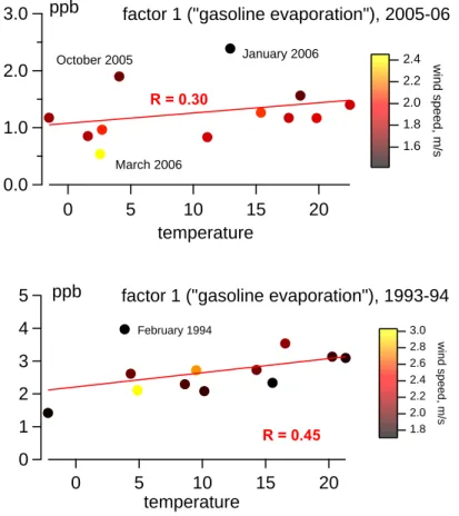
Modeled gasoline evaporation sources (factor 1) in 1993–1994 and in 2005–2006 are

20

positively correlated with temperatureR=0.45 and R=0.30 (Fig. 7), respectively, while the other factors (related to road traffic) show a different seasonal behavior, typically anti- or uncorrelated with temperature. In several cases, positive deviations from the linear regression slope (scores vs. temperature) coincide with low wind speed (Fig. 7), which is indicative for thermal inversions and pollutant accumulation (e.g. in February

25

1994, October 2005, and January 2006). This general dependence suggests that factor 1 in both data sets represents gasoline release via evaporation, during cold

ACPD

Full Screen / Esc

Printer-friendly Version Interactive Discussion

EGU starts and re-fueling rather than by warm-phase combustion. A positive correlation

with temperature might also be due to a combustion-related gasoline source that is active in summer (e.g. from ship traffic or from engines used at road works), but is rather unlikely due to relatively low correlations with the inorganic combustion tracers (Table 4).

5

The comparison of the PMF calculated gasoline factor with methyl-tert-buthyl-ether (MTBE) measured during two campaigns in 2005–2006 provides further evidence for an evaporative gasoline loss. Poulopoulos and Philippopoulos (2000) reported MTBE exhaust emission particularly during cold start and from evaporation. This is in agree-ment with other studies (e.g. MEF, 2001). Further, MTBE is neither synthesized in

10

Switzerland nor formed secondarily in the atmosphere, but exclusively used as a gaso-line additive with concentrations between 2% and 8% per volume (BAFU, 2002). The gasoline factor is strongly correlated with MTBE in summer as well as in winter (Fig. 8) and, therefore, likely represents evaporative gasoline loss and cold start phases. The slightly higher correlation found in summer (R=0.81) compared to winter (R=0.71) is

15

most probably due to larger temperature differences between day and night, which determine the amplitude of evaporative gasoline loss.

Gasoline and diesel fuel combustion.

As for gasoline evaporation, factors representing fuel combustion were also found in both data sets (factor 6). They exhibit a bimodal daily cycle with peaks in the morning

20

around 07:00 a.m. and in the evening at 09:00 p.m. in both data sets, as shown in Fig. 9 for the recent case (2005–2006). Typically, this temporal behavior is much more prominent on working days. A very similar pattern as found here was also reported for particulate emissions from incomplete fuel combustion at Zurich-Kaserne (Lanz et al., 2007). The strong dependence of the day of the week further supports findings

25

based on the hydrocarbon fingerprint of this factor (Sect. 3.3): diesel exhaust is a major contributor. A large fraction (∼66%, deduced from BAFU, 2000) of diesel-related total

ACPD

Full Screen / Esc

Printer-friendly Version Interactive Discussion

EGU hydrocarbons in 2000 was caused by the heavy-duty fleet (transport of goods), which

is not allowed to drive on weekends. Also commuter traffic is at a minimum, but the share of diesel passenger cars was and is still comparatively low in Switzerland (∼10%, HBEFA, 2004) compared to its neighboring states, as diesel taxes are relatively high and petroleum taxes rather low (Kunert and Kuhfeld, 2007). Note that the same diurnal

5

behavior was also found for other factors (e.g. solvents use; Sect. 3.4.4), but neither for ethane and propane sources (Sect. 3.4.3) nor for wood burning (Sect. 3.4.2).

Other traffic-related sources.

In 1993–1994, a similar factor to the gasoline evaporation source can be found (see Sect. 3.3.2), but due to the absence in 2005–2006 we hypothesize that this factor

10

represents gasoline combustion by cars without catalytic converters (factor 7, 1993– 1994). Recall that the fraction of non-catalyst vehicles was still in the order of one third of all passenger cars in the early 1990s (Sect. 3.3.2) and emissions were higher than from engines equipped with a catalytic converter. Today, this fraction is negligible: a large decrease in t-NMVOC (as well as in NOx) was found in measurements of the 15

Gubrist tunnel, which is located in the surroundings of Zurich (Colberg et al., 2005). Such tunnel studies do not cover cold start emissions and the large decrease was mainly attributed to the introduction of catalytic converters in the Swiss gasoline fleet. Therefore, no such factor could be resolved for the recently measured hydrocarbons (2005–2006). We will label this factor “earlier traffic source”.

20

3.4.2 Wood burning

Unlike the evaporative gasoline loss described in Sect. 3.4.1, factors representing wood burning activities are typically anti-correlated with temperature (i.e. increased domestic heating when outdoor temperatures are lower) and accumulate strongest during win-ter months that frequently are associated with temperature inversions (November to

ACPD

Full Screen / Esc

Printer-friendly Version Interactive Discussion

EGU February; Ruffieux et al., 2006) (Fig. 10). For this latter hydrocarbon source, no

signif-icant difference between daily emission pattern on working and non-working days can be observed (also when the data of different seasons are analyzed separately). It has been suspected that wood is mainly used for private, supplementary room heating in winter (Lanz et al., 2008), which is not connected to working days.

5

3.4.3 Ethane and propane sources

The ethane (2005–2006) and propane (1993–1994 and 2005–2006) dominated fac-tors generally exhibit a diurnal pattern different from other hydrocarbon sources, i.e. a bimodal daily cycle with maxima in the morning and late evening as found for fuel combustion (Sect. 3.4.1). In contrast, the diurnal patterns of the propane and ethane

10

dominated factors are generally characterized by an early morning maximum and a mid-afternoon minimum, which was observed for measured methane as well. This be-havior is shown for the 1993–1994 and 2005–2006 data in Fig. 11. Generally such a behavior is interpreted as accumulation during the night under a shallow inversion layer followed by reducing concentrations as the boundary layer expands during the

15

morning and early afternoon (e.g. Derwent et al., 2000). Concentrations are therefore highest when the boundary layer depth is smallest and lowest when the boundary layer depth is highest. This implies that these emission rates must be reasonably constant between day and night. The medians between midnight and 04:00 a.m. (small traffic contribution) increase linearly for the propane and ethane factor, but also for measured

20

methane in 2005–2006 (Fig. 11): an emission ratio for methane:ethane:propane of about 180:3:1 can be deduced. Natural gas leakage is an obvious candidate for the main urban source of these hydrocarbons, especially as a compositional ratio (per vol-ume) of 190(±129):3.7(±0.8):1 (methane:ethane:propane) can be deduced for trans-ported natural gas in Zurich (Erdgas Ostschweiz AG, Zurich, 2005/2006, unpublished

25

data). The uncertainties mainly reflect the variable gas mix, but also year-to-year vari-abilities. Natural gas consumption in [GWh] increased by 50% from 1992 to 2005 in Switzerland; it is typically more than four times higher in winter than in summer, which

ACPD

Full Screen / Esc

Printer-friendly Version Interactive Discussion

EGU would explain its correlation with SO₂. For the early data (1993–1994), the presence

of ethyne (Fig. 6) and a weak bimodal daily cycle (Fig. 11) point to the possibility that the ethane factor was then also influenced by incomplete combustion, possibly from residential (gas or oil) heating due to its yearly trend similar to that of wood burning (Fig. 10). It finally has to be noticed that factors 3 and 4 in both data sets

predom-5

inantly explain the variability (>60%) of ethane and propane, respectively. The nor-malized loadings of other hydrocarbons than ethane and propane (e.g. butane in the “propane” factor from 2005–2006) do not represent their explained variability, but are, in other words, partially floating species within the mentioned factors.

Due to their relatively long atmospheric lifetimes (days to weeks), propane and

10

ethane (also from other sources than gas leakage) tend to accumulate in the air. There-fore, we can not completely rule out that the factors “ethane” and “propane” may also represent aged VOC emissions as suspected by Buzcu and Fraser (2006). However, given the seasonal and diurnal patterns of those factors (Fig. 10 and Fig. 11) the con-tribution of processed VOC source emissions can not be of a major importance: for

15

aged and secondary organic aerosols (SOA) with similar lifetimes (days to weeks as the considered hydrocarbons) Lanz et al. (2007 and 2008) have calculated increasing concentrations in the early after-noon (due to elevated photochemical activity) and only a slight enhancement of their mean concentrations in the winter (5.3µg m−3) compared to summer (4.4µg m−3), as stronger accumulation and partitioning of volatile

precur-20

sors outweigh less solar radiation in wintertime (Strader et al., 1999). Furthermore, ethane and propane concentrations reported for European background air exhibit dif-ferent levels and time trends than the factors as calculated for the urban background here (also see Sect. 4). Firstly, the ethane factors, as an example, showed 3–8 times higher concentrations than reported for ethane in Finnish background air (Hakola et al.,

25

2006). Note that ethane is decomposed faster at mid latitudes than in Polar air (due to the temperature dependence of the ethane-OH reaction rate constant and [OH] lev-els). Secondly, we estimated that ethane and propane dominated factors, most likely representing natural gas leakage, slightly decreased by a factor of 1.3 from 1993–1994

ACPD

Full Screen / Esc

Printer-friendly Version Interactive Discussion

EGU to 2005–2006, whereas background ethane and propane showed increasing trends

between 1994 and 2003 (Hakola et al., 2006). We therefore conclude again that the hydrocarbon concentrations measured at the urban background of Zurich-Kaserne can not be significantly influenced by aged background air (also see Sect. 2.2.2).

3.4.4 Solvent usage

5

Acetates (belonging to the class of OVOCs) are commonly used solvents in industry (Legreid et al., 2007b). Also Niedojadlo et al. (2007) measured elevated acetate con-centrations close to industries in Wuppertal (Germany). A strong correlation was found between the sum of acetates (methyl-, ethyl, and butyl-) measured during two cam-paigns in 2005–2006 and the calculated solvent factor for 2005–2006 (Fig. 12). Lower

10

correlation of acetates in summertime (R=0.61) than in wintertime (R=0.70) is possibly due to secondary formation of acetates in the atmosphere, which is triggered by photo-chemistry. Further note that factor 2 was derived for two years of data; it nevertheless seems representative of weekly to daily variability of this hydrocarbon source.

3.5 Source contributions

15

Average source contributions as absolute concentrations [ppb] and relative [%] to the total mixing ratio of the 13 hydrocarbons were calculated for both data sets and sum-marized in Table 5.

3.5.1 Representativeness of the 13 hydrocarbons

The concentrations of the 13 hydrocarbons considered in this study accounted on

av-20

erage for 80–90% of the sum of all 22 NMHC species measured at this site since 2005. Aromatic C8hydrocarbons (m,p-xylene, o-xylene, and ethylbenzene) represent a major

fraction of that difference, accounting for more than 6% of the total concentration [ppb] of the 22 NMHCs. They were not measured in 1993 and 1994. A PMF analysis of the extended data set (2005–2006; comp. Sect. 2.2.5) revealed that those latter aromatics

ACPD

Full Screen / Esc

Printer-friendly Version Interactive Discussion

EGU will be attributed to solvent use (60%), fuel combustion (30%), gasoline evaporation

(5%), and wood burning (3%). The NMHCs plus the oxidized VOCs measured during three campaigns sum up to 73%–91% of the t-NMVOC concentrations determined by FID. For the earlier data (1993–1994), we estimate that NMHCs accounted for 62% and OVOCs for 13% of t-NMVOC (FID) on average. Today (2005–2006), the

rela-5

tive contributions to t-NMVOCs of the two measured classes is still 75% on average, but somewhat shifted towards the OVOCs (17%). Unlike the hydrocarbons used in this study, most OVOCs can be both directly released into the atmosphere or formed there secondarily. Furthermore they can be of anthropogenic as well as biogenic origin (Legreid et al., 2007b). We therefore conclude that the 13 hydrocarbons used in the

10

present study are representative for primary and anthropogenic hydrocarbon emissions in Zurich.

3.6 Hydrocarbon emission trends (1993–1994 vs. 2005–2006)

For most hydrocarbon sources (road traffic, solvent use, and wood combustion) de-creasing contributions by a factor 2–3 between 1993–1994 and 2005–2006 were

mod-15

eled (Table 5 and Fig. 13). This trend is also reflected by the decline of t-NMVOC mea-surements (Fig. 1) and vice versa. However, for ethane and propane sources (mainly city gas leakage), no such strong negative trend was found. In contrast, propane and ethane sources only decreased by a factor of 1.3 (but its consumption increased about 1.5 times). In Switzerland, steering taxes of about 2 Euro per kg VOC were enforced

20

in 1998. They are based on a black list of about 70 VOC species (e.g. toluene) or VOC classes (e.g. aromatic mixtures). Unlike most VOCs used in or as solvents, propane and ethane are not part of the black list (VOCV, 1997). This might explain the differ-ent trends for gas leakage hydrocarbons versus other sources. These results are in agreement with relatively constant methane concentrations measured in 1993–1994

25

and 2005–2006: ethane (1%–6%) and propane (∼1%) are minor components of natu-ral gas, which predominantly consists of methane (>90%). On the other hand, methane is emitted by other sources as well (e.g. incomplete combustion of fossil and non-fossil

ACPD

Full Screen / Esc

Printer-friendly Version Interactive Discussion

EGU materials) and therefore no perfect correlation can be expected.

3.6.1 Traffic-related sources and solvent use

The EMEP (Cooperative Programme for Monitoring and Evaluation of the Long-range Transmission of Air Pollutants in Europe) emission inventory for Switzerland (1993 ver-sus 2004) suggests that the most dominant sources, i.e. solvent use (115 Gg or 55% of

5

t-NMVOC in 1993) and road transport (63 Gg or 30% of t-NMVOC in 1993) decreased by a factor of two and three, respectively (Vestreng et al., 2006). Roughly the same relative decrease for road traffic and solvent use can be deduced from the data pre-sented in Table 5 and Fig. 13. However, we estimate that traffic is still an important VOC emission source accounting on average for 40% (1993–1994) and 29% (2005–2006)

10

of the measured hydrocarbon concentrations. In contrast, solvent usage contributed on average only to about 20% of the ambient hydrocarbon concentrations measured at Zurich-Kaserne.

For the 1993–1994 data Staehelin et al. (2001) have also found that road traffic con-tributes at least twice as much to ambient VOC concentrations than solvents, which is

15

in line with our findings. Thus, both studies disagree with the official Swiss emission inventory which claims that road traffic is a minor VOC source (contributing less than 20% to total VOCs, while solvent use would account for more than 50%; BAFU 2007). Vehicle emissions were limited by law since the 1980s, propagating the use of cata-lyst converters. Generally, road-traffic sources diminished by a factor of nearly three

20

between 1993–1994 and 2005–2006 (Fig. 13). However, the fuel combustion factor (strongly influenced by diesel contributions) only decreased by a factor of 1.3. For the diesel fleet, no catalysts have been enforced yet. This would also explain its rather similar hydrocarbon fingerprint found in 1993–1994 and in 2005–2006 (Sect. 3.3). On the other side, gasoline evaporation showed a decrease by a factor of 2.2. We can

25

explain this reduction of evaporative loss by the introduction of vapor recovery systems at Swiss gasoline stations during the late 1990s.

ACPD

Full Screen / Esc

Printer-friendly Version Interactive Discussion

EGU 3.6.2 Other trends

It is interesting to note that the modeled maximum wood burning emission in winter (January 2006 vs. February 1994) decreased by less than a factor 1.5, while mod-eled annual emissions decreased by a factor of 2.4. Therefore, the decrease of wood burning VOCs mainly results from reduced emissions in spring, summer, and autumn,

5

potentially caused by changes in agricultural and horticultural management.

4 Conclusions

Underlying factors of two year-long data sets of volatile hydrocarbons (C2–C7) were

de-scribed by multivariate receptor modeling (PMF) and related to different sources: fuel combustion, gasoline evaporation, solvent use, wood burning, and natural gas

leak-10

age. With different numbers of factors for the 1993–1994 (p=8) and 2005–2006 (p=6) data we accounted for the different emission situations prevailing in the two periods and thereby higher comparability between the factor analytical results was achieved. In contrast to a traditional CMB based analysis, no source profiles are imposed within the PMF approach to calculate the source activities, and the profiles are estimated

15

as well. In this way, we allowed for any changes in the nature and number of VOC source profiles, which obviously represents an advantage of an analysis based on PMF. We furthermore have provided evidence that yearly PMF factors are represen-tative for short-term source variability (days to weeks) by comparing factor scores to tracer OVOCs (methyl-tert-butyl-ether and acetates). We however can not rule out that

20

sources emitting widely variable hydrocarbon proportions, e.g. wood combustion (de-pending on burning conditions, temperatures etc.), may be underestimated by linear factor analysis.

To our knowledge it was not reported before that the number of dominating emission sources changed over time, which is however plausible due to large emission

reduc-25

ACPD

Full Screen / Esc

Printer-friendly Version Interactive Discussion

EGU traffic is in accordance with the measurements of a nearby road tunnel (Gubrist)

show-ing the successful introduction of catalytic converters in the Swiss road traffic fleet. Hydrocarbons from combustion sources (road traffic and wood burning) as well as solvent use decreased by a factor of two to three, while factors that mostly repre-sent natural gas leakage remained at relatively constant levels between 1993–1994

5

and 2005–2006. This general result is in line with conclusions drawn by Dollard et al. (2007) for similar sites (urban background) in the United Kingdom: while ethane concentrations pointing to natural gas leakage remained at constant levels between 1993 and 2004, a yearly decrease by −15% and −28% could be observed for vehicle exhaust tracing ethene and propene, respectively. A decrease of road traffic emissions

10

by factor of 2.8 during 12 years as estimated in this study is therefore also in line with findings from other European urban background locations. Note that the loss of natural gas relative to its transported amount also decreased by more than a factor of two as its consumption increased by 50% between 1992 and 2005.

In agreement with Niedojadlo et al. (2007; CMB analysis of ambient hydrocarbons

15

in a German city), we also found that solvent use is over-represented in European (Vestreng et al., 2006) as well as national (BAFU, 2007) emission inventories. We hypothesize that solvent VOCs used for industrial purposes were substituted by less toxic and oxidized VOCs; the proportion of OVOCs to t-NMVOCs measured at an urban background in Switzerland (Zurich-Kaserne) increased by 4% between 1993–1994 and

20

2005–2006. However, we believe that the disagreement between bottom-up (i.e. emis-sion inventories) and top-down approaches (i.e. modeling sources from field measure-ments) can only be partly explained by the fact that a certain amount of VOCs used in solvents are oxidized species; this aspect can not be covered by studies with a main focus on hydrocarbons. A minor issue is also the reduced transmission efficiencies for

25

long-chained and oxidized hydrocarbons that may adsorb on the surface of the inlet tubes to a greater extend. More importantly, many city centers in Europe and North-America today predominantly harbor service sectors, while manufacturing industries moved to suburban or remote places, which would indicate that Zurich is biased

to-ACPD

Full Screen / Esc

Printer-friendly Version Interactive Discussion

EGU wards traffic emissions.

Acknowledgements. The OVOC measurements were supported by the Swiss Federal Office for the Environment (FOEN). We thank U. Lohmann, A. Pr ´ev ˆot and H. Hell ´en for their valuable comments and suggestions which improved this paper. The earlier hydrocarbon data were provided by AWEL (Kanton Zurichs Department for Waste, Water, Energy, and Air). The current

5

VOC data are measured within the National Air Pollution Monitoring Network (NABEL). We are grateful to M. Hill for supporting the VOC measurements.

References

Anttila, P., Paatero, P., Tapper, U., and J ¨arvinen, O.: Source identification of bulk wet deposition in Finland by positive matrix factorization, Atmos. Environ., 29, 1705–1718, 1995.

10

BAFU: Luftschadstoff-Emissionen des Stassenverkehrs 1950–2020. Nachtrag. Schriftenreihe UMWELT Nr. 225, Swiss Federal Office for the Environment FOEN, Bern, 2000.

BAFU: Absch ¨atzung der Altlastenrelevanz von Methyl-tert-butylether (MTBE). Swiss Federal Office for the Environment FOEN, Bern, available at:

http://www.bafu.admin.ch/php/modules/shop/files/pdf/phpyeb9SE.pdf, 2002.

15

BAFU: Anthropogene VOC-Emissionen Schweiz 1998, 2001 und 2004, Swiss Federal Office for the Environment FOEN, Bern, available at:

http://www.bafu.admin.ch/voc/03756/03758/index.html?lang=de, 2007.

Barrefors, G. and Petersson, G.: Volatile hydrocarbons from domestic wood burning, Chemo-sphere, 30, 1551–1556, 1995.

20

Blifford, I. H. and Meeker, G. O.: A factor analysis model of large scale pollution, Atmos. Envi-ron., 1, 147–157, 1967.

Borbon, A., Coddeville, P., Locoge, N., and Galloo, J.-C.: Characterising sources and sinks of rural VOC in eastern France, Chemosphere, 57, 931–942, 2004.

Buset, K. C., Evans, G. J., Leaitch, W. R., Brook, J. R., Toom-Sauntry, D.: Use of advanced

25

receptor modelling for analysis of an intensive 5-week aerosol sampling campaign, Atmos. Environ., 40, Suppl 2, 482–499, 2006.

Buzcu, B. and Frazier, M. P.: Source identification and apportionment of volatile organic com-pounds in Houston, TX, Atmos. Environ., 40, 2385–2400, 2006.

ACPD

Full Screen / Esc

Printer-friendly Version Interactive Discussion

EGU Christensen, W. F., Schauer, J. J., and Lingwall, J. F.: Iterated confirmatory factor analysis for

pollution source apportionment, Environmetrics, 17, 663–681, 2006.

Colberg, C. A., Tona, B., Stahel, W. A., Meier, M., and Staehelin, J.: Comparison of a road traffic emission model (HBEFA) with emissions derived from measurements in the Gubrist road tunnel, Switzerland, Atmos. Environ., 39, 4703–4714, 2005.

5

Derwent, R. G., Davies, T. J., Delaney, M., Dollard, G. J., Field, R. A., Dumitrean, P., Nason, P. D., Jones, B. M. R., and Pepler, S. A.: Analysis and interpretation of the continuous hourly monitoring data for 26 C₂–C₈hydrocarbons at 12 United Kingdom sites during 1996, Atmos. Environ., 34, 297–312, 2000.

Dollard, G. J., Dumitrean, P., Telling, S., Dixon, J., and Derwent, R. G: Observed trends in

10

ambient concentrations of C₂–C₈hydrocarbons in the United Kingdom over the period from 1993 to 2004, Atmos. Environ., 41, 2559–2569, 2007.

Eggertsen, F. T. and Nelsen, F. M.: Gas chromatographic analysis of engine exhaust and at-mopshere. Determination of C₂–C₅hydrocarbons, Anal. Chem., 30, 1040–1043, 1958. Empa: Technischer Bericht zum Nationalen Beobachtungsnetz f ¨ur Luftfremdstoffe (NABEL),

15

available at:http://www.empa.ch/nabel, D ¨ubendorf, Switzerland, 2006.

Forster, P., Ramaswamy, V., Artaxo, P., Berntsen, T. , Betts, R., Fahey, D.W., Haywood, J., Lean, J., Lowe, D. C., Myhre, G., Nganga, J., Prinn, R., Raga, G., Schulz, M., and Van Dorland, R.: Changes in atmospheric constituents and in radiative forcing, in: Climate Change 2007: The Physical Science Basis. Contribution of Working Group I to the Fourth Assessment Report of

20

the Intergovernmental Panel on Climate Change, edited by: Solomon, S., Qin, D., Manning, M., Chen, Z., Marquis, M., Averyt, K. B., Tignor, M., and Miller, H. L., Cambridge University Press, Cambridge, United Kingdom and New York, NY, USA, 2007.

Fujita, E. M., Campbell, D. E., Zielinska, B., Sagebiel, J. C., Bowen, J. L., Goliff, W. S., Stock-well, W. S., and Lawson, D. R.: Diurnal and weekday variations in the source contributions of

25

ozone precursors in California’s South Coast Air Basin, J. Air Waste Manage., 53, 844–863, 2003.

Fuzzi, S., Andreae, M. O., Huebert, B. J., Kulmala, M., Bond, T. C., Boy, M., Doherty, S. J., Guenther, A., Kanakidou, M., Kawamura, K., Kerminen, V.-M., Lohmann, U., Rus-sell, L. M., and P ¨oschl, U.: Critical assessment of the current state of scientific

knowl-30

edge, terminology, and research needs concerning the role of organic aerosols in the at-mosphere, climate, and global change, Atmos. Chem. Phys., 6, 2017-2038, available at:

ACPD

Full Screen / Esc

Printer-friendly Version Interactive Discussion

EGU Hakola, H., Hell ´en, H., and Laurila, T.: Ten years of light hydrocarbons (C₂–C₆) concentration

measurements in background air in Finland, Atmos. Environ., 40, 3621–3630, 2006.

HBEFA: Handbuch f ¨ur Emissionsfaktoren des Strassenverkehrs (handbook of emission factors for road traffic), Umweltbundesamt Berlin, Bundesamt f ¨ur Umwelt, Wald und Landschaft Bern, Infras AG, Bern (published on CD-ROM, also available at: www.hbefa.net), 2004.

5

Hell ´en, H., Hakola, H., Pirjola, L., Laurila, T., and Pystynen, K.-H.: Ambient air concentrations, source profiles, and source apportionment of 71 Different C2–C10volatile organic compounds in urban and residential areas of Finland, Environ. Sci. Technol., 40, 103–108, 2006. Henry, R. C., Lewis, C. W., Hopke, P. K., and Williamson, H. J.: Review of receptor model

fundamentals, Atmos. Environ., 18, 1507–1515, 1984.

10

Henry, R. C.: Multivariate receptor modelling by N-dimensional edge detection, Chemometr. Intell. Lab., 65, 179–189, 2003.

Hopke, P. K: Recent developments in receptor modeling, Chemometr. Intell. Lab., 17, 255–265, 2003.

Jorquera, H. and Rappengl ¨uck, B.: Receptor modeling of ambient VOC at Santiago, Chile,

15

Atmos. Environ., 38, 4243–4263, 2004.

Junninen, H., Niska, H., Tuppurainen, K., Ruuskanen, J., and Kolehmainen, M.: Methods for imputation of missing values in air quality data sets, Atmos. Environ., 38, 2895–2907, 2004. Kunert, U. and Kuhfeld, H.: The diverse structures of passenger car taxation in Europe and the

EU Commissions proposal for reform, Transp. Policy, 14, 306–316, 2007.

20

Lanz, V. A., Alfarra, M. R., Baltensperger, U., Buchmann, B., Hueglin, C., and Prevot, A.S.H.: Source apportionment of submicron organic aerosols at an urban site by factor analyti-cal modelling of aerosol mass spectra, Atmos. Chem. Phys., 7, 1503-1522, available at:

http://www.atmos-chem-phys.net/7/1503/2007/, 2007.

Lanz, V. A., Alfarra, M. R., Baltensperger, U., Buchmann, B., Hueglin, C., Szidat, S., Wehrli,

25

M. N., Wacker, L., Weimer, S., Caseiro, A., Puxbaum, H. and Prevot, A. S. H.: Source attribution of submicron organic aerosols during wintertime inversions by advanced fac-tor analysis of aerosol mass spectra, Environ. Sci. Technol., 42, 214–220, available at:

http://pubs.acs.org/cgi-bin/abstract.cgi/esthag/asap/abs/es0707207.html, 2008.

Legreid, G., Reimann, S., Steinbacher, M., Staehelin, J., Young, D., and Stemmler, K:

Mea-30

surements of OVOCs and NMHCs in a Swiss highway tunnel for estimation of road transport emissions, Environ. Sci. Technol., 41, 7060–7066, 2007a.