Bayesian Calibration of Safety Codes Using
Data from Separate-and Integral Effects Tests
The MIT Faculty has made this article openly available. Please share
how this access benefits you. Your story matters.
Citation
Yurko, Joseph P., Jacopo Buongiorno, and Robert Youngblood.
"Bayesian Calibration of Safety Codes Using Data from
Separate-And Integral Effects Tests." Proceedings of the International
Meeting on Probabilistic Assessment and Analysis (PSA 2015),
Sun Valley, Idaho, USA, 26-30 April 2015. Vol. 1. American Nuclear
Society, 2015, pp. 718-727.
As Published
http://www.proceedings.com/27017.html
Publisher
American Nuclear Society
Version
Author's final manuscript
Citable link
http://hdl.handle.net/1721.1/107919
Terms of Use
Creative Commons Attribution-Noncommercial-Share Alike
BAYESIAN CALIBRATION OF SAFETY CODES USING DATA FROM SEPARATE-AND INTEGRAL EFFECTS TESTS
Joseph P. Yurko, Jacopo Buongiorno
MIT, 77 Massachusetts Avenue, Cambridge, MA, 02139, [email protected], [email protected] FPoliSolutions, LLC, 4618 Old William Penn Hwy, Murrysville, PA 15668, [email protected]
Robert Youngblood
INL, PO Box 1625, Idaho Falls, ID 83415-3870, [email protected]
Large-scale system codes for simulation of safety performance of nuclear plants may contain parameters whose values are not known very accurately. In order to be able to use the results of these simulation codes with confidence, it is important to learn how the uncertainty on the values of these parameters affects the output of the codes. New information from tests or operating experience is incorporated into safety codes by a process known as calibration, which reduces uncertainty in the output of the safety code, and thereby improves its support for decision-making. Modern analysis capabilities afford very significant improvements on classical ways of doing calibration, and the work reported here implements some of those improvements. The key innovation has come from development of safety code surrogate model (code emulator) construction and prediction algorithms. A surrogate is needed for calibration of plant-scale simulation codes because the multivariate nature of the problem (i.e., the need to adjust multiple uncertain parameters at once to fit multiple pieces of new information) calls for multiple evaluations of performance, which, for a computation-intensive model, makes calibration very computation-intensive. Use of a fast surrogate makes the calibration processes used here with Markov Chain Monte Carlo (MCMC) sampling feasible. Moreover, most traditional surrogates do not provide uncertainty information along with their predictions, but the Gaussian Process (GP) based code surrogates used here do. This improves the soundness of the code calibration process. Results are demonstrated on a simplified scenario with data from Separate and Integral Effect Tests.
I. INTRODUCTION
Bayesian inference provides a mathematically and statistically rigorous framework for solving inverse problems, which would otherwise be ill-posed or analytically intractable. Observational data can be used to calibrate1 computer model predictions and infer the
numerous parameters within the computer model. The resulting posterior distributions combine data with the expert judgment encoded within the prior distributions, thereby accounting for as much information as possible. However, implementing Bayesian calibration for safety analysis codes is very challenging. Because the posterior
distribution cannot be obtained analytically, approximate Bayesian inference with sampling is required. Markov Chain Monte Carlo (MCMC) sampling algorithms are very powerful and have become increasingly widespread over the last decade. 2 However, for even relatively “fast”
computer models practical implementation of Bayesian inference with MCMC would simply take too long. A computer model that takes 1 second to run but needs 105
MCMC samples would take over 27 hours to complete. Surrogate models (or emulators) that emulate the behavior of the input/output relationship of the computer model but are very computationally cheap allow MCMC sampling to be possible. An emulator that is 1000x faster than the computer model would need only 100 seconds to perform the same number of MCMC samples. As the computer model run time increases, the surrogate model becomes even more attractive because MCMC sampling would become impractically lengthy.
Ultimately, the goal is not simply to update the state of knowledge about some parameter values, but to use the updated parameters to better inform predictions on some system response. Observational data at various “levels” are therefore required. The lowest level or Separate Effect Tests (SETs) deals with a specific type of physical phenomenon or physical process. Calibrating a computer model with SET data calibrates the parameters associated with that specific physical process. Higher levels, or Integral Effect Tests (IETs), have multiple phenomena interacting together and are usually larger in scale. Calibrating a computer model with IET data alone may be quite difficult for many reasons, especially if the total number of parameters is very high. Incorporating the information from the SET data into the IET calibration would be able to improve the overall IET calibration process. The SET data should act to constrain the parameter distributions. 3 The SET model could be
calibrated first with the resulting posterior parameter distribution used to construct the prior for the IET model calibration. This work, however, calibrates the SET and IET models simultaneously. The benefit of the simultaneous approach is that a simple prior distribution can be used.
This work uses emulators to perform the simultaneous calibration of SET and IET models to their respective data. The methodology is demonstrated on a
simple channel pressure drop scenario. The SET deals with the specific pressure drop through one portion of the channel, namely the driver fuel bundle within the Experimental Breeder Reactor-II (EBR-II). The EBR-II was a sodium cooled fast reactor that operated for 30 years, performing a large number of important operational and safety analysis tests, before being shut down in 1994.12,16. The IET is the pressure drop over the entire
channel including the form loss at the inlet nozzle. Therefore, even though this demonstration requires only simple computer models, it still maintains the ingredients of the SET/IET calibration process. The IET model may not “know” the specific physics within the driver fuel bundle. The SET data will provide that information during the simultaneous calibration.
The rest of the paper is organized as follows: Section II discusses the specific type of emulator used in this work and how it is incorporated into the MCMC sampling, and the simultaneous calibration formulation. Section III describes the specific channel pressure drop SET and IET data and computer models, and Section IV provides the results.
II. EMULATOR-BASED BAYESIAN MODEL CALIBRATION
II.A Overview
Surrogate models can be used to approximate long-running computer codes to accomplish a variety of tasks. They are common in many engineering fields usually in the form of response surfaces and look-up tables.6 An
emulator is a specific type of surrogate model that
provides an estimate of its own uncertainty when making a prediction.4 An emulator is therefore a probabilistic
response surface which is a very convenient approach because the emulator’s contribution to the total uncertainty can be included in the Bayesian calibration process. An uncertain (noisy) emulator would therefore limit the parameter posterior precision, relative to calibrating the parameters using the long-running computer code itself.
A commonly-used emulator is the Gaussian Process (GP) model.4,5,6 The GP model is a Bayesian
non-parametric, non-linear model, and has been used successfully as an emulator in many engineering fields.6,7
Non-parametric refers to the fact that the GP model makes use of the training set in order to make a prediction. The training set is the set of computer code runs used to build, or, as the name implies, train the emulator. Parametric models, such as a best-fit line, never require the training set once the parameters within the model have been determined. Although computationally easier to manage, parametric models are not as flexible, and require the analyst to pre-specify the input/output relationship. Non-parametric statistical models, such as the GP, learn the input/output relationship
from the training data directly. The analyst must still pre-specify certain aspects of the GP, such as if the output is expected to be smooth or not, but in general the training data dictates the functional form rather than the analyst. For a comprehensive review of GP models see Ref. 5 and References 4, 6, and 7 for applying GP models to Bayesian model calibration of long-running computer codes.
However, the GP model has certain limitations. First, the GP does not scale very well to large amounts of data. The GP requires inversions of matrices that grow with increasing amounts of training data, which can be prohibitively slow for large amounts of data. Predicting multiple outputs is also challenging for the same reason, since the size of the matrices grows very quickly. Determining the training points is also not a trivial task. Training points that are too close together in the parameter space may cause the matrix which is required to be inverted to be singular or at least ill-conditioned. Naively using as many training points as possible may not help the GP, which may view some or many of the training points as effectively providing no new information relative to other points. This, too, can lead to the ill-conditioning issues.
Many different approaches have been adopted to overcome these issues. This work chose to adopt the Function Factorization with Gaussian Process (FFGP) Priors approach, a pattern-recognition style framework where the GP model is a piece of the overall statistical model.8 In the FFGP model, the training set is factored
into simpler functions. Each of the simpler functions is trained only by a fraction of the total training set. The pattern-recognition setup is therefore a dimensionality reduction technique since several smaller GP models are faster to work with than one very large GP. FFGP is a generalization of probabilistic Principal Component Analysis (PPCA) and Non-Negative Matrix Factorization (NMF).8 FFGP is also referred to as Gaussian Process
Factor Analysis (GPFA) by other authors in other fields.9
II.B Function Factorization with Gaussian Process (FFGP) Priors Model
II.B.1 Model Formulation
The main idea of function factorization (FF) is to approximate a complicated function, 𝑦(𝐱) , on a high-dimensional space, 𝒳 , by the sum of products of a number of simpler functions, 𝑓𝑖,𝑘(𝐱𝑖) , on lower
dimensional subspaces, 𝒳𝑖. The FF model is:
,
1 1 K I i k i k i y f
x x (1)In Eq. (1), I is the number of factors – patterns – and K is the number of different components within each factor.
The terminology used here is consistent with Schmidt’s in Ref. 7. The input, 𝐱 , is a vector with D-elements corresponding to the D-inputs to the problem. Each factor’s input, 𝐱𝑖, is a subset of the total input.
The difference between factor and component is easier to see when Eq. (1) is rewritten in matrix form. The training output data, 𝐘, is a matrix of size 𝑀 × 𝑁, where 𝑁 is the number of cases run and 𝑀 is the number of points taken per case. A case or case run denotes an evaluation of the computer model (the code) at a particular set of uncertain input parameter values. If the problem of interest was the analysis of a transient in a nuclear reactor, 𝑀 could be the number of points taken in time per case run. Factor 1 would be the time factor with 𝐱1 being a column vector of the 𝑀 points in time taken
per case run. If there was only 1 uncertain input parameter, 𝐱2 would be a vector of the 𝑁 different values
used to run the code 𝑁 times. In general, either factor’s input could be a matrix; the vectors were used here to describe the format. The entire set of training input values will be denoted as 𝐗 = {𝐱1, 𝐱2} , and the entire training dataset will be denoted as D X Y
,
. Withonly 1-component the FF-model becomes a matrix product of two vectors 𝐟1 and 𝐟2: Yf f1 2T . The
superscript T denotes the transpose of the vector. For more than one component, each factor is represented as a matrix instead of a vector. The columns within each factor’s matrix correspond to the individual components within that factor. For the 2-factor 2-component FF-model the factor matrices are 𝐅1= [𝐟1,1T , 𝐟1,2T ]
T
and 𝐅2=
[𝐟2,1T , 𝐟2,2T ] T
. The FF-model is then:
T 1 2
Y
F F
(2)The elements within each of the factor matrices are latent or hidden variables that must be learned from the training dataset. Performing Bayesian inference on the FF-model requires specification of a likelihood function between the training output data and the FF-model as well as the prior specification on each factor matrix. The likelihood function is assumed to be a simple Gaussian likelihood with likelihood noise (variance) 𝜎𝑛2 and mean
equal to the FF-model, 𝐅1𝐅2T.
The prior on each component within each factor is specified as a GP prior. Each GP prior is assumed to be a zero-mean GP with a squared-exponential (SE) covariance function. The SE covariance function is widely used in standard GP models because it is mathematically convenient (it is a Gaussian expression) and provides meaningful interpretation of the input/output relationship through a length scale hyperparameter. Each input has its own unique length scale which represents how far the values need to move (along a particular axis)
in each input space for the function values to become uncorrelated4. This formulation implements what is
known as automatic relevance determination (ARD) due to the fact that the inverse length scale determines how relevant the particular input is. If the length scale has a very large value, the covariance will become almost independent of that input.
Each factor’s covariance matrix requires evaluating the covariance function for all of that factor’s input pair combinations. The covariance matrix for factor 1 is therefore size 𝑀 × 𝑀 while the covariance matrix for factor 2 is size 𝑁 × 𝑁. This immediately shows how the FFGP is a dimensionality reduction technique compared to standard GP models where the covariance matrix size for all training points would be size 𝑁𝑀 × 𝑁𝑀. Each factor’s covariance matrix will be denoted asK and the i
set of all covariance function hyperparameters for that factor are denoted as 𝜙𝑖. The hyperparameters are
unknown and must be learned from the training data. The individual factors and components are all assumed independent a priori, therefore any covariance between components and factors results in the joint-posterior due to the contribution of their interaction within the likelihood function. All hyperparameters were also assumed to be independent and for simplicity were assumed to have improper “flat” hyperpriors. If the set of the hyperparameters is denoted as Ξ , the improper hyperprior is 𝑝(Ξ) ∝ 1. The probability model defining the joint-posterior distribution on all latent variables and hyperparameters is given in detail in Ref. 11.
II.B.2 Emulator Training
As shown in Ref. 5, building standard GP models requires learning the various hyperparameters within the statistical model. The FFGP emulator adds an additional layer to the training because hyperparameters as well as latent variables must be learned simultaneously to fully specify the emulator.
Following Schmidt in Ref. 8, the Hamiltonian Monte Carlo (HMC) MCMC scheme was used to build the FFGP emulator. The HMC is a very powerful MCMC algorithm that accounts for gradient information to suppress the randomness of a proposal. See References 8, 10, and 17 for detailed discussions on HMC. The HMC algorithm is ideal for situations with a very large number of highly correlated variables, as is the case with sampling the latent variables presently.
This work has several key differences from Schmidt’s training algorithm in Ref. 8, to simplify the implementation and increase the execution speed. Following Ch. 5 in Ref. 17, the latent variables and hyperparameter sampling were split into a “Gibbs-like” procedure. A single iteration of the MCMC scheme first samples the latent variables given the hyperparameters, then samples the hyperparameters given the latent
variables. The latent variables were sampled with HMC, but the hyperparameters can now be sampled from a simpler MCMC algorithm such as the Random-Walk-Metropolis (RWM) sampler. Although less efficient compared to the HMC scheme, the RWM performed adequately for this work.
The next key difference relative to Schmidt’s training algorithm was to use an empirical Bayes approach and fix the hyperparameters as point estimates. Fixing the hyperparameters as point estimates neglects their impact on the emulator uncertainty; however, the empirical Bayes approach is far less computationally expensive and is commonly used with GP models.5 The empirical Bayes
approach used here is slightly different than most because the hyperparameters are fixed at the end of MCMC sampling rather than determined by an optimization scheme. The hyperparameter point estimates are denoted as Ξ̂. Once fixed, the HMC algorithm is restarted, but now the hyperparameters are considered known.
The end result of the HMC algorithm is a potentially very large number of samples of all of the latent variables. One last simplification relative to Schmidt’s setup was to summarize the latent variable posteriors as Gaussians. Their posterior means and covariance matrices were empirically estimated from the posterior samples. All of the latent variables are denoted in stacked vector notation as f and the empirically estimated means of the latent variables are 𝔼[𝐟̂|𝒟, Ξ̂]. The empirically estimated covariance matrix of all the latent variables is cov[𝐟̂|𝒟, Ξ̂]. As will be shown in the next section, this assumption greatly simplified making predictions with the FFGP emulator and ultimately provided a very useful approximation that aided the overall goal of emulator-based Bayesian model calibration.
II.B.3 Posterior Predictions
Once the FFGP emulator is built, it can be used to make predictions at new input values, not used in the training set. A prediction consists of two steps: first, make a prediction in the latent factor space; then, combine the factor predictions together to make a prediction on the output directly. A latent space posterior prediction is very straightforward following MVN theory.8,9 Predictions on
the output space are made by assuming the FF-model predictive distribution is a Gaussian. The FF-model predictive mean and variance are estimated using the laws of total expectation and variance with details given in Ref. 11. Due to the assumptions made to evaluate the posterior predictions analytically, the FF-model predictions are labeled as approximate posterior predictions.
II.C Emulator-Modified Likelihood Function
The FF-model approximate posterior predictive distribution is used to modify the likelihood function
between the observational data and the uncertain input parameters. The observational data will be assumed to in vector form labeled asy . The computer code prediction o
will also be labeled in vector form asy x
cv,
, with x cvdenoting a set of control variables controlled by the experimenters,4 while 𝜃 is the set of uncertain input
parameters of interest. The control variables can also be the time the data was taken if the experiment of interest is a transient. Typically, in Bayesian calibration of computer models, the computer code prediction is used as a (non-linear) mapping function within the likelihood function. The posterior on 𝜃 is then given as:
p
|yo
p
yo|y x
cv o, ,
p
(3)The subscript “o” on the control variable locations refers to the fact that the computer predictions are made at the same control variable “locations” as the observational data. The likelihood function in Eq. (3) could however be written in a “hierarchical-like” fashion with the “total” likelihood broken into two parts as given in Eq. (4):
p
y
, |
y
o
p
y y
o|
p
y x
|
cv,
p
(4) The first part on the right hand side of Eq. (4) is the likelihood between the observational data and the computer prediction p
yo|y while the second is the
likelihood between the computer prediction and the inputs
| cv,
p y x . The likelihood between the observational data and the computer prediction is simply the assumed likelihood model for the experiment. This work assumes a simple factorizable Gaussian likelihood function with known measurement error (variance) 2
ò , which is
common in practice due to its simplicity. The likelihood between the computer prediction and the inputs is much more complicated to specify however and is most likely impossible to analytically determine for safety analyses codes in the nuclear industry. However, thanks to the emulator framework, this likelihood can be approximated by the emulator posterior predictive distribution.
Denoting the FF-model prediction as 𝐇∗, the joint
posterior between the FF-model prediction and the uncertain inputs 𝜃 is:
* * * , ˆ , | , , ˆ | | cv o, , , p p p p o o H y y H H x D D (5)By assuming the FF-model prediction is Gaussian, the FF-model prediction can be integrated out when likelihood between the observational data and computer
prediction is also Gaussian. This leads to the emulator-modified calibration process where the emulator-emulator-modified likelihood function relates the uncertain inputs directly to the observational data. The uncertain input posterior after the FF-model posterior prediction has been integrated out is:
p
|yo, ,D ˆ
p
yo|
xcv o,,
, ,Dˆ
p
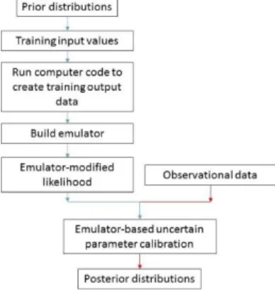
(6)The FFGP-modified likelihood function is used in place of the conventional likelihood function in a MCMC sampling scheme. The emulator-based Bayesian model calibration process is summarized by a flowchart depicted in Fig. 1 below.
Fig. 1. Emulator-based Bayesian model calibration flow chart.
II.D Emulator-Based Simultaneous Bayesian Calibration of Multiple Models
In order to calibrate multiple models simultaneously, the emulator-modified likelihood function needs to be modified slightly. In general terms, the total number of models will be denoted as 𝑍 with the total set of observational data for all 𝑍 experiments labeled as 𝕐𝐨=
{𝐲𝐨,𝑧}𝑧 𝑍
with corresponding computer model predictions 𝕐 = {𝐲𝑧}𝑧𝑍. These 𝑍 models could be allowed to be
correlated; however, this work assumed that the models are uncorrelated. The complete likelihood structure between all models simply takes a factorized form:
,
1 | | Z z z z p p
O yo y Y Y (7)The convenience of this assumption is that each of the 𝑍 models’ individual likelihood functions can be approximated by that specific model’s own emulator-modified likelihood function.
III. CHANNEL PRESSURE DROP DEMONSTRATION
III.A Overview
To demonstrate simultaneous emulator-based calibration, a flow channel pressure calibration scenario is presented. This was a piece of a larger emulator-based calibration of RELAP5 as discussed in Ref. 11. There are two models, a SET model of a bundle-specific pressure drop through the driver fuel region of the core in EBR-II. The driver fuel region is the middle portion of the entire core channel which sandwiches the EBR-II driver fuel between the upper and lower blanket.12 The core channel
IET model therefore includes the lower blanket, driver fuel, and upper blanket, as well as the core channel inlet nozzle form. The SET model therefore informs one specific portion of the IET model.
The experimental data are values of pressure drop at various mass flow rates through the channel. The control variable is therefore the inlet mass flow rate rather than time, which was the example used throughout the discussion of the FFGP emulator.
Both the SET and IET models are generated using RELAP5. The set of uncertain parameters involve the RELAP5 user-defined friction factor correlation which allows specifying turbulent coefficients, A and B, the turbulent exponent, C and the laminar flow shape factor
S
17. The turbulent user defined friction factor
correlation is:
T (Re)C
f A B (8)
The leading coefficient A was pre-set to be zero and was considered known. Together, B and C are referred to as the turbulent parameters. In the laminar flow regime, the friction factor correlation is:
64 Re L S f (9)
In Eqs. (8) and (9), Re is the Reynolds number and the friction factor is denoted as f (not to be confused with the emulator latent variables). Within the transition flow regime, RELAP5 interpolates between the turbulent and laminar friction factors.18 The user defined friction factor
inputs were specified for each region within the channel. The upper and lower blankets share the same set of inputs, while the driver fuel region has its own set of B, C, and values. Including the core channel inlet nozzle S loss coefficient, the total number of uncertain input parameters to the IET RELAP5 model is 7 while the SET RELAP5 model has only 3 uncertain inputs.
Although a lot of EBR-II data exist, the bundle-specific SET is a “pseudo” SET. The observational data are in fact generated from an empirical correlation rather than coming from a true experiment. Therefore, the SET can be viewed as updating the various uncertain inputs in the RELAP5 user-defined friction factor correlation to match physical phenomena not present in the default list of friction factor correlations within RELAP5. EBR-II had a tight light wire-wrapped bundle within the driver fuel region.12 An appropriate friction factor correlation
for this design is the Cheng & Todreas wire-wrapped bundle average friction factor correlation.13 Once the
Cheng & Todreas friction factor is computed for the desired mass flow rate, the pressure drop over the length of the driver fuel bundle is computed. A total of 25 “pseudo” data points were used.
For the core channel IET data, the data are taken from Gapalakrishnan & Gillette (1973) (Ref. 14). The core channel pressure drop includes the effect of the inlet nozzle form loss. It is difficult to determine whether the data presented in Ref. 14 are real measured experimental data and not simply the results of an empirical correlation derived from scaled water tests. However, the present IET and SET model calibration demonstration is illustrative of the entire process, whether the core channel pressure drop is real or synthetic. Fig. 2 below shows the data taken directly from Ref. 14. Since the pressure drop are read off of Fig. 2, only 6 data points were taken for the IET “pseudo” data.
Fig. 2. Core Channel IET Pressure Drop Data from Ref. 13.
III.C RELAP5 Model Descriptions
The SET and IET RELAP5 models are very similar. Both are simply channels built using 1-D pipe RELAP components. The SET model consists of one pipe channel to represent the driver fuel bundle. Single volumes are connected at the inlet and outlet of the driver fuel channel which are connected to the inlet mass flow and outlet pressure boundary conditions (BCs). Those single volumes have wall friction turned off and are used to calculate the total pressure drop across the pipe
component of interest. Fig. 3 provides an illustration of the RELAP5 SET model.
Fig. 3. RELAP5 SET Model Illustration.
The core channel IET RELAP5 model is very similar to the SET model in Fig. 3. Two additional 1-D pipe components were attached to the driver fuel pipe component, one to represent the lower blanket and the other to represent the upper blanket. Additionally, the inlet nozzle loss coefficient is added to the junction that connects volume 200 in Fig. 3 to the lower blanket pipe component. Both the SET and IET RELAP5 models are steady-state models.
IV. RESULTS
In this work, all of the uncertain parameters are given uniform prior distributions between their assumed minimum and maximum values. In general, the choice of prior for epistemically uncertain variables is controversial, but in the present application, it is seen that some of the variables are determined extremely well by the data alone. The min/max values were assumed to be multiples of the McAdams friction factor correlation coefficient and exponent for B and C and a multiple of 1 for the laminar shape factor. The core channel inlet nozzle loss coefficient bounding values were determined by varying its value from a set of trial runs.
All of the posterior input parameter results will be shown on a scaled basis. The scaled value of 0 corresponds to the prior minimum bound while the scaled value of 1 is the prior maximum bound. In the scaled values the priors were all uniform between 0 and 1.
The uniform prior bounding values were used as the bounding values to generate the training sets. Therefore the uniform prior prevented the MCMC sampling scheme from jumping outside of the training set bounding values. Future work will improve on the treatment of cases where the search “wants” to go outside the prior assessed variable ranges.
IV.A Bundle-Specific SET Calibration Results
The SET RELAP5 model has 3 uncertain input parameters. Along with the control variable – the inlet mass flow rate - a total of 4 inputs exist to the SET RELAP5 model. A general rule of thumb in building a standard GP model is to use 10 training points per input.4
Even though the FFGP emulator is being used and not the standard GP emulator, an additional 10 case runs were conservatively added, giving a total of 50 case runs. The
specific uncertain input parameter values were chosen using Latin Hypercube Sampling (LHS). Fifteen control variable locations were used for each case. Thus, with 50 cases and 15 control variable locations, a total of 750 RELAP runs were made. The training dataset is shown in grey along with the Cheng & Todreas “pseudo” data as red error bars in Fig. 4. The “pseudo” data were assumed to have a measurement error such that 95% of the probability was covered by +33% around the mean data value of the first data point. This error (variance) was then assumed constant for each of the 25 data points. The error bars are very small in Fig. 4. The pressure drop across the bundle is plotted against the scaled inlet mass flow rate, where 1 corresponds to the max inlet mass flow rate. Each RELAP5 run took roughly 2 seconds to complete, thus it took about 25 minutes to generate the entire FFGP training set. However, all of the RELAP5 runs were made in series for simplicity. The training set could be run in parallel, which would significantly shorten the training set build time.
Fig. 4. SET RELAP5 Model Training Set.
A total of 3 types of FFGP emulators were built: the 2-factor 1-component, 2-component and 3-component emulators. The FFGP training algorithm used a total of
5
3 10 samples, but as described in Sect. II.B.2, the Gibbs-like portion of the sampling was discarded after the hyperparameters were fixed. The Gibbs-like portion used
5
10 samples; then, after restarting, the next 105samples were treated as “burn-in” on the training latent variable samples. Therefore, only 105samples were stored as the final posterior training latent variable samples used to estimate the empirical mean and covariance matrix. The three FFGP emulator types were trained on the same personal computer. The 1-component FFGP emulator took roughly 1.5 minutes to train while the 3-component FFGP emulator took 2.3 minutes to train. Building the emulators therefore adds very little computational overhead compared to simply generating the training set.
Only the 2-factor, 2-component FFGP emulator calibrated results will be shown. The FFGP-modified likelihood function was incorporated into an Adaptive Metropolis (AM) MCMC algorithm15 and a total of 5
10
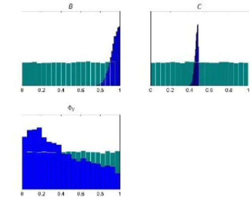
samples were drawn. The calibrated posterior predictions are shown in Fig. 5 while the calibrated scaled uncertain input histograms are shown in Fig. 6. Because the “pseudo” data were so precise, the calibrated posterior predictions have very little uncertainty. The scaled parameter histograms show the prior histograms in green and the posterior histograms in blue. It is interesting that the posterior on C, the exponent acting on the friction factor correlation, has its uncertainty shrunk around the prior mean (the McAdams value), while the posterior on
B, the coefficient on the Reynolds number is shifted
closer to the prior maximum bounding value. This is the situation to be dealt with in the future work previously mentioned.
The posterior mode of the laminar shape factor, Φ𝑆,
is shifted closer to the prior lower bound, but is not changed substantially from its uniform prior. This is representative of the fact that the variation in the data cannot be “explained” by the variation in Φ𝑆, resulting in
little change in the posterior relative to the prior. The turbulent exponent C, has the greatest reduction in variance relative to its prior. The turbulent exponent therefore “explains” the variation in the data the most, which makes physical sense.
Fig. 5. SET calibrated posterior predictions relative to the “pseudo” data.
Fig. 6. SET only calibrated posterior histograms The histograms in Fig. 6 are the MCMC approximate
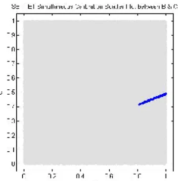
sampling scheme provides access to the approximate joint posterior distribution between the uncertain parameters. Although more difficult to display, the joint posterior distribution captures any data-induced correlation between the uncertain parameters. A scatter plot is used to show the correlation between the B and C parameters in FKG below. The gray background is the scatter plot from the independent uniform prior distributions which illustrates no correlation a priori. The scatter plot of the posterior samples is displayed in blue which shows the very strong linearly correlation between B and C. The very strong correlation between the turbulent coefficient and exponent was induced completely by the data, even though the prior distributions were assumed independent. Scatter plots between the turbulent parameters and the laminar shape factor are not given here, but very little posterior correlation exists.
Fig. 7. SET only turbulent parameter scatter plot.
Table 1 shows the computational times for all 3 FFGP-based Bayesian calibration schemes. The values in parentheses provide include the time to generate the training set. It is very clear that the emulator is much faster to evaluate compared to the RELAP5 model. However the effective number of RELAP5 runs shown in the last column of Table 1 assumes the 2 second run time per case. A single MCMC run that compares all 25 “pseudo” data points would therefore require 25 separate RELAP5 runs. If those could be run in parallel, then the slowest FFGP emulator is over 3000x faster than if RELAP5 was used directly for MCMC sampling. However, if the RELAP5 calculations had to be made in series, a single MCMC iteration would take roughly 50 seconds to complete. The slowest FFGP emulator would be over 75000x faster than this in-series RELAP5-based approach.
Table 1. SET emulator computational times.
FFGP type Total emulator-based calibration time [min]
Effective number of RELAP5 1-component 2.22 (27.22) 66 (816) 2-component 2.89 (27.89) 86 (836) 3-component 3.36 (28.36) 100 (850)
IV.B Core Channel IET Calibration Results
The same process was followed for the core channel IET RELAP5 calibration. However, since the IET model has 7 uncertain inputs, a total of 100 case runs were used. Fifteen control variable locations (number of inlet mass flow rate values per case run) were maintained. A single case run now took roughly 3 seconds, so it took roughly 75 minutes to generate the entire training set, which is shown in Fig. 8.
Fig. 8. IET RELAP5 Model Training Set
Four emulator types were trained for the IET model, 2-factor, 1-component through 4-components. Each was built following the same process as the SET FFGP emulators. Training took between 2.2 and 3.6 minutes for the 4 FFGP emulators. The 2-factor, 3-component FFGP based calibration results are shown in
Fig. 9 and Fig. 10. The effect of the emulator uncertainty is easier to see in
Fig. 9 than Fig. 5. The blue lines are the 5th, 25th,
50th, 75th and 95th quantile lines of the calibrated posterior
predictive mean. The green band is the total calibrated predictive uncertainty band, accounting for the emulator’s contribution to the predictive variance. The edge of the green band is +2 standard deviations around the mean of the predictive means. The blue lines therefore represent what the emulator thinks the computer model (RELAP5) would predict. The further the edge of the green band gets from the last of the blue lines represents the emulator contributing a large amount of uncertainty to the calibration process.
Fig. 9. IET-calibrated posterior predictions relative to the “pseudo” data.
Just as in the SET calibration process, the FFGP emulators added very little computational overhead compared to simply generating the training set. The total emulator-based calibration time excluding generating the training set was between 1.5 minutes and 4 minutes for the IET FFGP emulators. Generating the training set (running RELAP5) therefore took roughly 95% of the total computational run time for the slowest FFGP emulator.
The important part of the IET FFGP-based calibration results, however, is that the top row of posterior histograms in Fig. 10 are different from the three posterior histograms shown in Fig. 6. These are the same three uncertain input parameters but they have vastly different posterior distributions. The histograms in the middle row of Fig. 10 are the blanket parameters and the last histogram is for the inlet nozzle loss coefficient. The IET model essentially explains all of the variability in the data by the inlet nozzle loss coefficient. The IET model by itself has no other piece of information to suggest that any of the posterior values are unphysical for the other six uncertain parameters. This point is made even clearer by examining a scatter plot of the driver fuel bundle turbulent parameters, as shown in Fig. 11. Comparing Fig. 11 to Fig. 7 clearly shows that the IET data by itself cannot capture the strong linear correlation between the B and C parameters. The SET data must therefore be included in the calibration process to provide that information.
Fig. 10. IET-only calibrated scaled posterior histograms.
IV.C Simultaneous Calibration Results
The 2-factor, 2-component FFGP SET emulator and the 2-factor, 3-component FFGP IET emulator were used together to simultaneously calibrate the 7 uncertain parameters. A total of 2 10 5 MCMC samples were drawn with the first half discarded as burn-in. The simultaneous calibration posterior histograms are shown in Fig. 12. The results are just as expected: the two dominant parameters from the SET model, the Reynolds number coefficient and exponent in the friction factor correlation are nearly identical to their corresponding
Fig. 11. IET-only turbulent parameter scatter plot.
SET-only calibration results. The inlet nozzle loss posterior is likewise similar to the IET-only calibration result. The blanket friction parameters (the middle row of histograms in Fig. 12) are also similar to the IET-only calibration results in Fig. 10. Those input parameters do not influence the SET model so it makes sense that including the SET model has minimal impact on their posterior, since the inlet nozzle loss coefficient completely dominates the core channel pressure drop.
Fig. 12. Simultaneous calibration scaled posterior histograms.
The histograms in Fig. 12 approximate the simultaneously calibrated marginal distributions. However, fully comparing the calibration results requires comparing the resulting joint distributions. The scatter plot between the driver fuel turbulent parameters as determined by the simultaneous calibration process is shown in Fig. 13. Comparing Fig. 13 to Fig. 7 clearly shows the simultaneous calibration results capture the very strong linear trend between the turbulent parameters.
A single MCMC iteration was only slightly slower than the sum of the individual MCMC iterations giving the calibration time to be roughly 4.67 minutes. The computational expense is dominated by the generation of the training sets. This work for simplicity generated the
Fig. 13. Simultaneous calibrated turbulent parameter scatter plot.
training sets in series, which took 25 minutes and 75 minutes for the SET and IET RELAP5 models, respectively. Even if all of the RELAP5 models could be run in parallel, the computational time is limited by the time to run a single IET RELAP5 model case, which is roughly 3 seconds. Simultaneous calibration with 2 10 5 MCMC samples would have then taken roughly 7 days to complete. The emulator-based simultaneous calibration with both training sets generated in series took less than 3 hours to complete.
V. SUMMARY AND CONCLUSIONS
Although conceptually simple, this channel pressure drop scenario illustrated the steps involved in performing emulator-based model calibration in a practical situation. Multiple computer models were synthesized with multiple experimental data to calibrate the uncertain input parameters within the computer models. Without the emulators, MCMC would simply not be a computationally feasible option, as seen in the execution time differences between the emulator and the RELAP5 models.
ACKNOWLEDGMENTS
This work was supported through the INL National Universities Consortium (NUC) Program under DOE Idaho Operations Office Contract DE-AC07-05ID14517.
REFERENCES
1. OBERKAMPF, W.L. and C. J. ROY, Verification
and Validation in Scientific Computing
(Cambridge University Press, Cambridge, UK, 2010). 2. D.L. KELLY and C.L. SMITH, “Bayesian Inference in Probabilistic Risk Assessment: The Current State of the Art,” Reliability Engineering and System Safety, vol. 94, pp. 628-643, 2009.
3. R.NELSON, C. UNAL, J. STEWART, B. WILLIAMS, “Using Error and Uncertainty
Quantification to Verify and Validate Modeling and Simulation,” LANL, Nov. 2010, LA-UR-10-06125. 4. Managing Uncertainty in Complex Models. [Online].
Available: http://www.mucm.ac.uk/
5. C. RASMUSSEN and C.K. WILLIAMS, Gaussian
Processes in Machine Learning, Springer, 2004.
6. A.J. KEANE and P.B. NAIR, Computational
Approaches for Aerospace Design: The Pursuit of Excellence, John-Wiley & Sons, 2005.
7. D. HIGDON, J. GATTIKER, B. WILLIAMS, and M. RIGHTLEY, “Computer Model Calibration Using High-Dimensional Output” Journal of the American
Statistical Association, vol. 103, no. 482, June 2008.
8. M. SCMIDT, “Function Factorization Using Warped Gaussian Processes,” in Proceedings of the
Twenty-Sixth International Conference on Machine Learning.
New York: ACM, 2009.
9. J. LUTTINEN and A.T. ILIN, “Variational Gaussian-Process Factor Analysis for Modeling Spatio-Temporal Data,” in Advances in Neural Information
Processing Systems 22, Y. Bengio, D. Schuurmans, J.
Lafferty, C. Williams, and A. Culotta, Eds. Curran Associates, Inc., 2009, pp. 1177-1185.
10. K.P. MURPHY, Machine Learning: A Probabilistic
Perspective. Cambridge, MA: MIT Press, 2012.
11. J.P. YURKO, Uncertainty Quantification in Safety
Codes Using a Bayesian Approach with Data from Separate and Integral Effect Tests. Dissertation, MIT.
Cambridge, MA, 2014.
12. L. KOCH, W. LOEHNESTEIN, and H.O.
MONSON, “Addendum to Hazard Summary Report Experimental Breeder Reactor-II (EBR-II),” Argonne National Laboratory, Tech. Rep., 1962.
13. N. TODREAS and M. KAZIMI, Nuclear Systems
Volume I: Thermal Hydraulic Fundamentals, Second Edition. CRC Press, 2011, vol. 1.
14. A. GOPALAKRISHNAN and J. GILLETTE, “EBRFLOW-A Computer Program for Predicting the Coolant Flow Distribution in the Experimental Breeder Reactor-II,” Nuclear Technology, vol. 17, pp. 205-216, March 1973.
15. H. HAARIO, E. SAKSMAN, and J. TAMMINEN, “An Adaptive Metropolis Algorithm,” Bernoulli, vol. 7, pp. 223-242, 1998.
16. G. GOLDEN, H. PLANCHON, J. SACKETT, and R. SINGER, “Evolution of Thermal-Hydraulics Testing in EBR-II”, Nuclear Engineering and Design, vol. 101, pp. 3-12, 1987.
17. S. BROOKS, A. GELMAN, G.L. JONES, X.L. MENG, Handbook of Markov Chain Monte Carlo, Chapman and Hall/CRC, 2011.
18. RELAP5-3D Code Manual, Rev. 2.2 ed. INEEL-EXT-98-00834, 2003.