A Complete Readout Chain
of the ATLAS Tile Calorimeter for the HL-LHC:
from FATALIC Front-End Electronics
to Signal Reconstruction
Sergey Senkin, on behalf of the ATLAS Tile Calorimeter System
Laboratoire de Physique de Clermont-Ferrand Campus Universitaire des C´ezeaux
4 Avenue Blaise Pascal 63178 Aubi`ere cedex, France Email: sergey.senkin@cern.ch
Abstract—The ATLAS Collaboration has started a vast
pro-gramme of upgrades in the context of high-luminosity LHC (HL-LHC) foreseen in 2024. We present here one of the front-end readout options, an ASIC called FATALIC, proposed for the high-luminosity phase LHC upgrade of the ATLAS Tile Calorimeter. Based on a 130 nm CMOS technology, FATALIC performs the complete signal processing, including amplification, shaping and digitisation. We describe the full characterisation of FATALIC and also the Optimal Filtering signal reconstruction method adapted to fully exploit the FATALIC three-range layout. Additionally we present the resolution performance of the whole chain measured using the charge injection system designed for calibration. Finally we discuss the results of the signal reconstruction used on real data collected during a preliminary beam test at CERN.
I. INTRODUCTION
ATLAS [1] is one of two general-purpose experiments at the Large Hadron Collider (LHC) at CERN. It is designed to realise the full discovery potential and the vast range of physics opportunities provided by the LHC. The Tile Calorimeter (TileCal) [2] is the hadronic calorimeter covering the central region of the ATLAS detector, as can be seen on Fig. 1. It is essential for the measurement of hadrons, jets, tau leptons and missing transverse energy.
The upgrade of the LHC to the high-luminosity phase (HL-LHC) [3] foreseen in 2024 will provide invaluable opportu-nities for the search for new physics beyond the Standard Model, as well as the detailed studies of the electroweak symmetry breaking mechanism and precise measurements of the properties of recently discovered Higgs boson. The ATLAS Collaboration has started an extensive programme of HL-LHC upgrades for every sub-detector, including TileCal. The current readout electronics of TileCal must be upgraded to comply with the new specifications aiming for the future operating conditions.
The ASIC described in this document, named Front-end ATlAs tiLe Integrated Circuit (FATALIC) [4], has been de-veloped to fulfil the requirements of the HL-LHC upgrade.
Fig. 1. A cut-away view of the ATLAS calorimeters. The TileCal comprises a central barrel region with pseudorapidity range of |η| < 1.7, and two extended barrel regions providing coverage up to |η| < 2.4.
It is one of the front-end readout options proposed for the upgrade of TileCal, based on a 130 nm CMOS technology and designed for the complete processing of the signal delivered by each Photomultiplier-Tube (PMT), including amplification, shaping and digitisation.
The document is structured as follows. The overview of the FATALIC layout as well as the main progress stages of its development and the performance measurements are given in Section II. The signal reconstruction aspects are described in Section III. Subsection III-A gives an overview of the Optimal Filtering algorithm which is used to reconstruct the amplitude and time of the signal is described. The specific details of application of this algorithm to FATALIC pulses are described in subsection III-B. Finally, the results of the signal reconstruction used on real data collected during a preliminary beam test at CERN are shown in Section IV, and a short conclusion is given in Section V.
II. FATALICLAYOUT
The front-end readout system designed for the HL-LHC upgrade has to abide by stringent requirements, an overview of which is given in Table I. In order to comply with them and particularly with the large dynamic range requirement of 25 fC to 1.2 nC, a three-gain layout has been adopted for FATALIC.
TABLE I
HL-LHC REQUIREMENTS FOR THEFRONT-ENDREADOUT
Technology 0.13 µm CMOS GlobalFoundries Number of channel per ASIC 1
Polarity negative Dynamic range in charge Q = 25 fC – 1.2 nC Dynamic range in current peak Q = 1.25µA – 60 mA
Rise time of the current peak tr= 4 ns
Fall time of the current peak tf = 36 ns
Noise (RMS) < 12fC Power as low as possible Power supply 1.6 V
Output word of 12 bits at 40 MHz
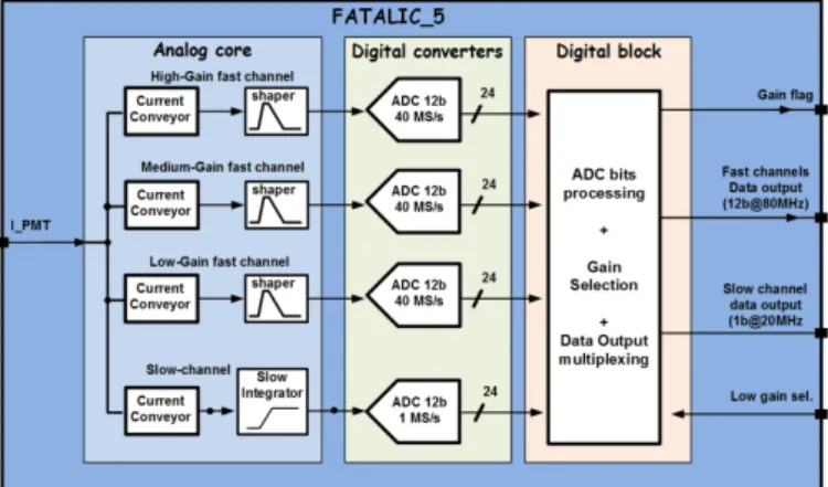
The overall layout of the latest ASIC iteration, FATALIC5, is shown in Fig. 2. The first stage of FATALIC is a current conveyor which splits the input signal into three ranges with gain ratios of 1, 8 and 64. Each current conveyor output is followed by a shaper and a dedicated pipelined 12-bit Analogue-to-Digital Converter (ADC) operating at 40 MHz. As a result, the analogue signal from the physics events is digitised at the ADC output, which in case for FATALIC is integrated in the ASIC itself. Due to bandwidth limitations, only two gains are forwarded to the output. Auto-selection of the data to be transmitted is performed between the high and the low gains, while the medium gain data are always included. This auto-selection is performed digitally inside the chip based on the saturation of the most sensitive channel. Fig. 3 shows an example of an analogue signal at the FATALIC shaper output (using a digital scope) and a digitised event at the ADC output, both shown for a muon event.
Fig. 2. Block diagram of the latest design of FATALIC ASIC.
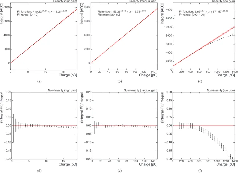
The dynamic performance of the whole chain is measured in terms of resolution using the dedicated charge injection system designed for calibration. Fig. 4 shows the linearity results for the three gains of the previous FATALIC ASIC, FATALIC4b. It can be seen that the non-linearity is contained within 2% for the high and medium gains over their whole range. However, saturation is observed for the low gain starting at around 600 pC.
This drawback has been addressed in FATALIC5. The improvement of the linearity, particularly for the low gain, is achieved at the input stage (the current conveyor) by reducing the impact of the high input currents (about 60 mA for a charge of 1.2 nC) on the Grid-Source voltage variations of the input transistor. Use of larger transistors allows these variations to be reduced by almost one order of magnitude. Fig. 5 gives the linearity results for the latest FATALIC5 design, obtained using simulation. The non-linearity is now better than 1% over the whole dynamic range for all gains.
Another improvement implemented in FATALIC5 is the addition of the slow channel (Fig. 2), necessary for the measurement of low current. This measurement is needed for the absolute detector calibration with radioactive caesium source, which produces a known but low signal. While the three previously described channels have integration times of 25 ns (the LHC clock period), the slow channel has a 100 µs time constant inside the integrator. For this channel, the digitisation is performed over 1.2 µs by the ADC, and the integration time is 10 ms. Larger integration times are accessible by digital means, when requested. The fast and slow channels are always DC coupled, and the current is split by allocating 20% to the fast channel, and 80% to the slow one. The optimisation of this ratio is obtained using simulation. The FATALIC5 design has been recently sent to foundry, and its first performance tests are planned for July 2017.
III. SIGNALRECONSTRUCTION
A. Optimal Filtering in TileCal
Optimal Filtering (OF) is a method of reconstructing the amplitude of an analogue signal from its digital samples. It is currently used in TileCal as a main reconstruction method, and is also envisaged to be used in the future with one of the front-end readout options implemented. The method is well-documented in the designated ATLAS note [5], and here we describe the main principle behind Optimal Filtering.
The digitised samples, such as those at the output of FATALIC, can be expressed as:
Si= p + Ag(ti+ τ ) + ni (1)
where p is the signal pedestal, A is the true amplitude, g(t) is the normalized reference pulse shape (taken from the shaper circuit, which provides a stable and well-defined pulse shape),
τ is the phase between the expected and measured pulse times,
and ni is the noise term, which is typically modelled by
a Gaussian distribution if only electronic noise is present. In order to make the phase τ an output parameter of the
Not reviewed, for internal cir culation only
ATLAS Phase-II Upgrade
Tile Calorimeter System Draft 0.1, December 6, 2016 01:16Initial Design Review
Figure 102: Left: Analog signal (shaper output) of a muon event. Right: Digital signal (ADC output) of a muon event through the whole chain
counts for the Low gain. It is too much, in particular in the digital auto-selection of the High or
1354
Low gain, even though the last design (FATALIC 4b) is using the Low gain information where
1355
the dispersion is smaller than in the High gain channel. Due to technological fluctuations,
1356
these dispersions will be corrected in the next development of FATALIC 5. Let us remind
1357
that once the pedestal will be adjusted, they will be stable because there is no AC coupling
1358
in between the PMT and the ADCs. Dynamic performances are measured by using first the
1359
charge injection system, then light-emitting diodes on a dedicated test bench. Figure 103 shows the linearity results for the three gains by using the CIS.
1360
The non-linearity is within 2% for the High and Medium gains over their whole range, but saturation starts for the Low gain above 600 pC. However, the linearity is better when
1361
injecting light pulses to PMTs. Indeed simulations show that a too large capacitance in the
1362
CIS contributes to the non-linearity behavior. Linearity corrections could be done off-line, but
1363
hardware improvements are preferred both at the CIS level and in the conveyor architecture
1364
of the next FATALIC 5 design. Taking benefit from the low noise level in the pulse mode,
1365
it was foreseen to replace the standard current integration for the Cesium calibrations (and
1366
over larger durations for the Luminosity estimates) by a digital summation of the samples
1367
at 40 MHz. Unfortunately, the tests failed because of the strong noise increase at the very
1368
low frequencies corresponding to these durations, where the noise varies like 2 nA/
p
GHz at1369
100 nA, while at higher frequencies the thermal noise is dominant, as shown in Figure 104.
1370
That implies a new development with an additional slow channel inside FATALIC based on a
1371
current measurement over 10 ms that will be described in the design of FATALIC 5. For larger
1372
integration times, in particular in the Luminosity scans, digital means of these measurements will be performed.
1373
First test beam results showed strange pedestal shapes of every channel (Figure 105), either enlarged with respect to the previous measurements or having counts outside the ideal shape.
1374
Estimated through the pedestal rms, this effect is all the more sizeable that the PMT channel
1375
is far from its corresponding FPGA on the Main Board. The explanation is very simple: the bit
1376
transmission of FATALIC data towards the FPGA is disturbed by the track length, and so the quoted rms values did not correspond to the expected electronic noise as shown in Figure 101.
1377
The design of FATALIC 5 will overcome this problem by changing the electronic trans-mission of digitized data. Nevertheless, data were taken with particles. Figure 106 shows,
1378
4.6 The FATALIC Option 85
(a) Not reviewed, for internal cir culation only
ATLAS Phase-II Upgrade
Tile Calorimeter System Draft 0.1, December 6, 2016 01:16Initial Design Review
Figure 102: Left: Analog signal (shaper output) of a muon event. Right: Digital signal (ADC output)
of a muon event through the whole chain
counts for the Low gain. It is too much, in particular in the digital auto-selection of the High or
1354
Low gain, even though the last design (FATALIC 4b) is using the Low gain information where
1355
the dispersion is smaller than in the High gain channel. Due to technological fluctuations,
1356
these dispersions will be corrected in the next development of FATALIC 5. Let us remind
1357
that once the pedestal will be adjusted, they will be stable because there is no AC coupling
1358
in between the PMT and the ADCs. Dynamic performances are measured by using first the
1359
charge injection system, then light-emitting diodes on a dedicated test bench. Figure 103
shows the linearity results for the three gains by using the CIS.
1360
The non-linearity is within 2% for the High and Medium gains over their whole range,
but saturation starts for the Low gain above 600 pC. However, the linearity is better when
1361
injecting light pulses to PMTs. Indeed simulations show that a too large capacitance in the
1362
CIS contributes to the non-linearity behavior. Linearity corrections could be done off-line, but
1363
hardware improvements are preferred both at the CIS level and in the conveyor architecture
1364
of the next FATALIC 5 design. Taking benefit from the low noise level in the pulse mode,
1365
it was foreseen to replace the standard current integration for the Cesium calibrations (and
1366
over larger durations for the Luminosity estimates) by a digital summation of the samples
1367
at 40 MHz. Unfortunately, the tests failed because of the strong noise increase at the very
1368
low frequencies corresponding to these durations, where the noise varies like 2 nA/
p
GHz at
1369
100 nA, while at higher frequencies the thermal noise is dominant, as shown in Figure 104.
1370
That implies a new development with an additional slow channel inside FATALIC based on a
1371
current measurement over 10 ms that will be described in the design of FATALIC 5. For larger
1372
integration times, in particular in the Luminosity scans, digital means of these measurements
will be performed.
1373
First test beam results showed strange pedestal shapes of every channel (Figure 105), either
enlarged with respect to the previous measurements or having counts outside the ideal shape.
1374
Estimated through the pedestal rms, this effect is all the more sizeable that the PMT channel
1375
is far from its corresponding FPGA on the Main Board. The explanation is very simple: the bit
1376
transmission of FATALIC data towards the FPGA is disturbed by the track length, and so the
quoted rms values did not correspond to the expected electronic noise as shown in Figure 101.
1377
The design of FATALIC 5 will overcome this problem by changing the electronic
trans-mission of digitized data. Nevertheless, data were taken with particles. Figure 106 shows,
1378
4.6 The FATALIC Option 85
(b)
Fig. 3. (a) Analogue signal (shaper output) of a muon event. (b) Digital signal (ADC output) of a muon event through the whole chain.
0 5 10 15 Charge [pC] 0 2000 4000 6000 8000 Integ ral
[ADC] Fit function: 410.22±1.04× x − 8.21±6.28
Fit range: [0, 10]
Linearity (high gain)
(a) 0 20 40 60 80 100 120 140 Charge [pC] 0 2000 4000 6000 8000 Integ ral
[ADC] Fit function: 52.22±0.12× x − 2.72±6.06
Fit range: [20, 80]
Linearity (medium gain)
(b) 0 200 400 600 800 1000 1200 1400 Charge [pC] 0 2000 4000 6000 8000 10000 12000 14000 Integ ral
[ADC] Fit function: 6.62±0.1⇥ x + 871.57±29.62
Fit range: [200, 400]
Linearity (low gain)
(c) 0 5 10 15 Charge [pC] −0.20 −0.15 −0.10 −0.05 0.00 0.05 0.10 0.15 0.20 (Integ ral-Fit)/Integ ral
Non-linearity (high gain)
(d) 0 20 40 60 80 100 120 140 Charge [pC] −0.20 −0.15 −0.10 −0.05 0.00 0.05 0.10 0.15 0.20 (Integ ral-Fit)/Integ ral
Non-linearity (medium gain)
(e) 0 200 400 600 800 1000 1200 1400 Charge [pC] −0.20 −0.15 −0.10 −0.05 0.00 0.05 0.10 0.15 0.20 (Integ ral-Fit)/Integ ral
Non-linearity (low gain)
(f) Fig. 4. Linearity and non-linearity of the previous design (FATALIC4b) for (a, d) high, (b, e) medium and (c, f) low gains.
II. FATALICLAYOUT
The front-end readout system designed for the HL-LHC upgrade has to abide by stringent requirements, an overview of which is given in Table I. In order to comply with them and particularly with the large dynamic range requirement of 25 fC to 1.2 nC, a three-gain layout has been adopted for FATALIC.
TABLE I
HL-LHC REQUIREMENTS FOR THEFRONT-ENDREADOUT
Technology 0.13 µm CMOS GlobalFoundries Number of channel per ASIC 1
Polarity negative Dynamic range in charge Q = 25 fC – 1.2 nC Dynamic range in current peak Q = 1.25µA – 60 mA
Rise time of the current peak tr= 4 ns
Fall time of the current peak tf = 36 ns
Noise (RMS) < 12fC Power as low as possible Power supply 1.6 V
Output word of 12 bits at 40 MHz
The overall layout of the latest ASIC iteration, FATALIC5, is shown in Fig. 2. The first stage of FATALIC is a current conveyor which splits the input signal into three ranges with gain ratios of 1, 8 and 64. Each current conveyor output is followed by a shaper and a dedicated pipelined 12-bit Analogue-to-Digital Converter (ADC) operating at 40 MHz. As a result, the analogue signal from the physics events is digitised at the ADC output, which in case for FATALIC is integrated in the ASIC itself. Due to bandwidth limitations, only two gains are forwarded to the output. Auto-selection of the data to be transmitted is performed between the high and the low gains, while the medium gain data are always included. This auto-selection is performed digitally inside the chip based on the saturation of the most sensitive channel. Fig. 3 shows an example of an analogue signal at the FATALIC shaper output (using a digital scope) and a digitised event at the ADC output, both shown for a muon event.
Fig. 2. Block diagram of the latest design of FATALIC ASIC.
The dynamic performance of the whole chain is measured in terms of resolution using the dedicated charge injection system designed for calibration. Fig. 4 shows the linearity results for the three gains of the previous FATALIC ASIC, FATALIC4b. It can be seen that the non-linearity is contained within 2% for the high and medium gains over their whole range. However, saturation is observed for the low gain starting at around 600 pC.
This drawback has been addressed in FATALIC5. The improvement of the linearity, particularly for the low gain, is achieved at the input stage (the current conveyor) by reducing the impact of the high input currents (about 60 mA for a charge of 1.2 nC) on the Grid-Source voltage variations of the input transistor. Use of larger transistors allows these variations to be reduced by almost one order of magnitude. Fig. 5 gives the linearity results for the latest FATALIC5 design, obtained using simulation. The non-linearity is now better than 1% over the whole dynamic range for all gains.
Another improvement implemented in FATALIC5 is the addition of the slow channel (Fig. 2), necessary for the measurement of low current. This measurement is needed for the absolute detector calibration with radioactive caesium source, which produces a known but low signal. While the three previously described channels have integration times of 25 ns (the LHC clock period), the slow channel has a 100 µs time constant inside the integrator. For this channel, the digitisation is performed over 1.2 µs by the ADC, and the integration time is 10 ms. Larger integration times are accessible by digital means, when requested. The fast and slow channels are always DC coupled, and the current is split by allocating 20% to the fast channel, and 80% to the slow one. The optimisation of this ratio is obtained using simulation. The FATALIC5 design has been recently sent to foundry, and its first performance tests are planned for July 2017.
III. SIGNALRECONSTRUCTION
A. Optimal Filtering in TileCal
Optimal Filtering (OF) is a method of reconstructing the amplitude of an analogue signal from its digital samples. It is currently used in TileCal as a main reconstruction method, and is also envisaged to be used in the future with one of the front-end readout options implemented. The method is well-documented in the designated ATLAS note [5], and here we describe the main principle behind Optimal Filtering.
The digitised samples, such as those at the output of FATALIC, can be expressed as:
Si= p + Ag(ti+ τ ) + ni (1)
where p is the signal pedestal, A is the true amplitude, g(t) is the normalized reference pulse shape (taken from the shaper circuit, which provides a stable and well-defined pulse shape),
τis the phase between the expected and measured pulse times,
and ni is the noise term, which is typically modelled by
a Gaussian distribution if only electronic noise is present. In order to make the phase τ an output parameter of the
Not reviewed, for internal cir culation only
ATLAS Phase-II Upgrade
Tile Calorimeter System Draft 0.1, December 6, 2016 01:16Initial Design Review
Figure 102: Left: Analog signal (shaper output) of a muon event. Right: Digital signal (ADC output) of a muon event through the whole chain
counts for the Low gain. It is too much, in particular in the digital auto-selection of the High or
1354
Low gain, even though the last design (FATALIC 4b) is using the Low gain information where
1355
the dispersion is smaller than in the High gain channel. Due to technological fluctuations,
1356
these dispersions will be corrected in the next development of FATALIC 5. Let us remind
1357
that once the pedestal will be adjusted, they will be stable because there is no AC coupling
1358
in between the PMT and the ADCs. Dynamic performances are measured by using first the
1359
charge injection system, then light-emitting diodes on a dedicated test bench. Figure 103 shows the linearity results for the three gains by using the CIS.
1360
The non-linearity is within 2% for the High and Medium gains over their whole range, but saturation starts for the Low gain above 600 pC. However, the linearity is better when
1361
injecting light pulses to PMTs. Indeed simulations show that a too large capacitance in the
1362
CIS contributes to the non-linearity behavior. Linearity corrections could be done off-line, but
1363
hardware improvements are preferred both at the CIS level and in the conveyor architecture
1364
of the next FATALIC 5 design. Taking benefit from the low noise level in the pulse mode,
1365
it was foreseen to replace the standard current integration for the Cesium calibrations (and
1366
over larger durations for the Luminosity estimates) by a digital summation of the samples
1367
at 40 MHz. Unfortunately, the tests failed because of the strong noise increase at the very
1368
low frequencies corresponding to these durations, where the noise varies like 2 nA/
p
GHz at1369
100 nA, while at higher frequencies the thermal noise is dominant, as shown in Figure 104.
1370
That implies a new development with an additional slow channel inside FATALIC based on a
1371
current measurement over 10 ms that will be described in the design of FATALIC 5. For larger
1372
integration times, in particular in the Luminosity scans, digital means of these measurements will be performed.
1373
First test beam results showed strange pedestal shapes of every channel (Figure 105), either enlarged with respect to the previous measurements or having counts outside the ideal shape.
1374
Estimated through the pedestal rms, this effect is all the more sizeable that the PMT channel
1375
is far from its corresponding FPGA on the Main Board. The explanation is very simple: the bit
1376
transmission of FATALIC data towards the FPGA is disturbed by the track length, and so the quoted rms values did not correspond to the expected electronic noise as shown in Figure 101.
1377
The design of FATALIC 5 will overcome this problem by changing the electronic trans-mission of digitized data. Nevertheless, data were taken with particles. Figure 106 shows,
1378
4.6 The FATALIC Option 85
(a) Not reviewed, for internal cir culation only
ATLAS Phase-II Upgrade
Tile Calorimeter System Draft 0.1, December 6, 2016 01:16Initial Design Review
Figure 102: Left: Analog signal (shaper output) of a muon event. Right: Digital signal (ADC output)
of a muon event through the whole chain
counts for the Low gain. It is too much, in particular in the digital auto-selection of the High or
1354
Low gain, even though the last design (FATALIC 4b) is using the Low gain information where
1355
the dispersion is smaller than in the High gain channel. Due to technological fluctuations,
1356
these dispersions will be corrected in the next development of FATALIC 5. Let us remind
1357
that once the pedestal will be adjusted, they will be stable because there is no AC coupling
1358
in between the PMT and the ADCs. Dynamic performances are measured by using first the
1359
charge injection system, then light-emitting diodes on a dedicated test bench. Figure 103
shows the linearity results for the three gains by using the CIS.
1360
The non-linearity is within 2% for the High and Medium gains over their whole range,
but saturation starts for the Low gain above 600 pC. However, the linearity is better when
1361
injecting light pulses to PMTs. Indeed simulations show that a too large capacitance in the
1362
CIS contributes to the non-linearity behavior. Linearity corrections could be done off-line, but
1363
hardware improvements are preferred both at the CIS level and in the conveyor architecture
1364
of the next FATALIC 5 design. Taking benefit from the low noise level in the pulse mode,
1365
it was foreseen to replace the standard current integration for the Cesium calibrations (and
1366
over larger durations for the Luminosity estimates) by a digital summation of the samples
1367
at 40 MHz. Unfortunately, the tests failed because of the strong noise increase at the very
1368
low frequencies corresponding to these durations, where the noise varies like 2 nA/
p
GHz at
1369
100 nA, while at higher frequencies the thermal noise is dominant, as shown in Figure 104.
1370
That implies a new development with an additional slow channel inside FATALIC based on a
1371
current measurement over 10 ms that will be described in the design of FATALIC 5. For larger
1372
integration times, in particular in the Luminosity scans, digital means of these measurements
will be performed.
1373
First test beam results showed strange pedestal shapes of every channel (Figure 105), either
enlarged with respect to the previous measurements or having counts outside the ideal shape.
1374
Estimated through the pedestal rms, this effect is all the more sizeable that the PMT channel
1375
is far from its corresponding FPGA on the Main Board. The explanation is very simple: the bit
1376
transmission of FATALIC data towards the FPGA is disturbed by the track length, and so the
quoted rms values did not correspond to the expected electronic noise as shown in Figure 101.
1377
The design of FATALIC 5 will overcome this problem by changing the electronic
trans-mission of digitized data. Nevertheless, data were taken with particles. Figure 106 shows,
1378
4.6 The FATALIC Option 85
(b)
Fig. 3. (a) Analogue signal (shaper output) of a muon event. (b) Digital signal (ADC output) of a muon event through the whole chain.
0 5 10 15 Charge [pC] 0 2000 4000 6000 8000 Integ ral
[ADC] Fit function: 410.22±1.04× x − 8.21±6.28
Fit range: [0, 10]
Linearity (high gain)
(a) 0 20 40 60 80 100 120 140 Charge [pC] 0 2000 4000 6000 8000 Integ ral
[ADC] Fit function: 52.22±0.12× x − 2.72±6.06
Fit range: [20, 80]
Linearity (medium gain)
(b) 0 200 400 600 800 1000 1200 1400 Charge [pC] 0 2000 4000 6000 8000 10000 12000 14000 Integ ral
[ADC] Fit function: 6.62±0.1⇥ x + 871.57±29.62
Fit range: [200, 400]
Linearity (low gain)
(c) 0 5 10 15 Charge [pC] −0.20 −0.15 −0.10 −0.05 0.00 0.05 0.10 0.15 0.20 (Integ ral-Fit)/Integ ral
Non-linearity (high gain)
(d) 0 20 40 60 80 100 120 140 Charge [pC] −0.20 −0.15 −0.10 −0.05 0.00 0.05 0.10 0.15 0.20 (Integ ral-Fit)/Integ ral
Non-linearity (medium gain)
(e) 0 200 400 600 800 1000 1200 1400 Charge [pC] −0.20 −0.15 −0.10 −0.05 0.00 0.05 0.10 0.15 0.20 (Integ ral-Fit)/Integ ral
Non-linearity (low gain)
(f) Fig. 4. Linearity and non-linearity of the previous design (FATALIC4b) for (a, d) high, (b, e) medium and (c, f) low gains.
0 5 10 15 20 25
Max Shaper Signal [V]
0 0.2 0.4 0.6 0.8 1 1.2 1.4 g_h_10pF_800ohms Simulation slope = 0.05749 offset = -0.00 g_h_10pF_800ohms Input charge [pC] 0 5 10 15 20 25 (mV) ∆ 2 − 1 − 0 1 2 (a) 0 20 40 60 80 100 120 140 160 180 200
Max Shaper Signal [V]
0 0.2 0.4 0.6 0.8 1 1.2 1.4 g_m_40pF_200ohms_4V Simulation slope = 0.00697 offset = -0.01 g_m_40pF_200ohms_4V Input charge [pC] 0 20 40 60 80 100 120 140 160 180 200 (mV) ∆ 20 − 10 − 0 10 20 (b) 0 200 400 600 800 1000 1200
Max Shaper Signal [V]
0 0.2 0.4 0.6 0.8 1 1.2 1.4 g_l_320pF_25ohms_4V Simulation slope = 0.00078 offset = -0.03 g_l_320pF_25ohms_4V Input charge [pC] 0 200 400 600 800 1000 1200 (mV) ∆ 20 − 10 − 0 10 20 (c)
Fig. 5. Linearity of the latest design (FATALIC5) for (a) high, (b) medium and (c) low gains (simulation results). ∆(mV) in the bottom plots indicates the absolute difference between the shaper signal and the linear fit. 1 mV corresponds to 0.1% relative difference with respect to the whole dynamic range.
algorithm, the dependence of Si on τ can be linearised via
Taylor’s expansion at first order:
Si p + Ag(ti)− Aτg (ti) + ni= p + Agi− Aτgi + ni (2)
Three sets of free parameters ai, biand ciare defined, called
OF weights, such as:
A = N i=1 aiSi = N i=1 ai Si (3)
where N is the number of samples.
The OF procedure aims at minimizing the variance of the linear combinations of these parameters subject to a set of con-straints. These constraints lead to a set of linear equations [5], which prompt the derivation of the OF weights and hence the amplitude, pulse time and pedestal can be calculated.
B. Optimal Filtering application to FATALIC
1) Analytical pulse shape: In order to validate the principle
of the Optimal Filtering reconstruction method, a study was performed with the reference pulse shape taken from the analytic function of the following form:
V (t) = Vnorm×Erf (1− e
−t−tupτup ) + 1
2 × e
−t−tdownτdown + V
0 (4)
where Vnorm is the normalisation parameter, Erf is the
Gaus-sian error function [6], tup and τup are the pulse rise time
parameters, tdown and τdownare the pulse fall time parameters,
and V0 is the pedestal. This function approximates the pulse
shape measured with scope (Fig. 3, a), and is represented in Fig. 6 where it is compared with the scope output. The shape is clearly asymmetrical, making it different from the pulses of other front-end options (e.g. 3in1 [7]).
2) Construction of pulses: Before the OF method is tested
in real conditions, it is important to validate its performance using known sampled pulses. In this study, to produce a sam-pled digitised pulse, the input reference pulse shape (Fig. 6) is normalised and sampled every 25 ns which is the LHC clock period. Then the normalised pulse is multiplied by the energy
0 20 40 60 80 100 120 140 160 180 200 Voltage [mV] 600 − 500 − 400 − 300 − 200 − 100 − 0 100 Integral = -9.93 V.s = 1.60 mV > 2 <(data-model) ) = ( -383 , -0.7) mV 0 , V norm (V = ( 44 , 8.0) ns up ) τ (t , = ( 54 , 9.3) ns down ) τ (t , data model = 8.8 ns up t ∆ = 32.7 ns down t ∆ PMT output Time [ns] 0 20 40 60 80 100 120 140 160 180 200 [%] max / V ∆ 4 − 2 − 0 2 4 0 20 40 60 80 100 120 140 160 180 200 Voltage [mV] 0 50 100 150 200 250 Integral = 10.00 V.s = 1.47 mV > 2 <(data-model) ) = ( 173 , -0.1) mV 0 , V norm (V = ( 74 , 13.7) ns up ) τ (t , = ( 97 , 31.7) ns down ) τ (t , data model = 18.8 ns up t ∆ = 103.2 ns down t ∆ Shaper output Time [ns] 0 20 40 60 80 100 120 140 160 180 200 [%] max / V ∆ 4 − 2 − 0 2 4
Fig. 6. Analytical pulse shape (“model”) compared with the scope output (“data”).
factor and added with a fixed typical pedestal value. The energy factor is obtained from a known conversion rate of the input charge to the energy deposited in a TileCal cell, which is taken from a uniform distribution. The noise factor is then added for each sample independently, uncorrelated between samples in the first approximation. The noise factors for each sample are considered as independent Gaussian distributions, RMS of which are later on referred to as noise levels.
As shown above, FATALIC layout comprises three different gains covering three dynamic ranges. While the medium gain is always present, high or low gain is selected depending on the saturation of either gain. For the purpose of validating the OF method with the analytical pulse shape whilst also simulating the gain switch behaviour, an effective digitised pulse is constructed by using the medium and alternative gain based on the following criteria:
• if both high and medium gains are saturated (sHG> 4095
ADC, sMG> 4095ADC):
– seff = 64 ×sLG ADC
• if only high gain is saturated, and medium gain is not
(sHG> 4095ADC, sMG< 4095ADC):
– seff = 8 ×sMG ADC
• if neither high nor medium gain are saturated (sHG <
4095ADC, sMG< 4095ADC):
– seff = sHG ADC
Here sHG, sMG, sLGcorrespond to the signal output yields of
the high, medium and low gains, and seff is the resulting signal
of an effective digitised pulse encoded in 18 bits. Fig. 7 shows the digitised pulses for the medium gain, alternative gain, and the effective 18-bit digitised pulse.
3) Performance results: The main performance criteria
pre-sented here is the pulse energy resolution, defined as follows: ∆E
E =
EOF− Etrue
Etrue , (5)
where Etrue is the true energy, and EOF is the energy
reconstructed by the Optimal Filtering method.
The energy resolution plots for a typical LHC energy range from 100 MeV to 1.5 TeV are shown in Fig. 8 for two different scenarios: with and without the electronic noise. For the latter case, the typical noise levels are considered: 3.5 ADC (∼8.4 fC) for the high gain, 1.5 ADC (∼29 fC) for the medium gain, and 1.5 ADC (∼230 fC) for the low gain. It can be seen that the energy resolution is kept within percentage level across four orders of magnitude of the signal energy.
IV. RESULTS WITH REAL DATA
For the final validation of the Optimal Filtering method and the whole chain of the FATALIC readout system, the signal reconstruction performance was tested with real data collected during a preliminary beam test at CERN [8]. In Fig. 9 (a) the OF method is compared with the flat estimation method, which is the basic energy reconstruction corresponding to the simple summation of digitised samples. Clearly, the Optimal Filtering reconstruction provides a significant improvement of energy resolution compared to the simple summation approach. Fig. 9 (b) shows the two-dimensional plot of the energy reconstructed using the OF method for muon events recorded by two different channels of a single cell, and the expected correlation is observed accordingly.
V. CONCLUSION
We have presented an overview and performance of the FATALIC front-end readout option of the TileCal High-Luminosity LHC upgrade foreseen in 2024. The character-isation of the full chain was shown, as well as the signal reconstruction was validated. The Optimal Filtering signal reconstruction method was introduced, its adaptation to fully exploit the FATALIC three-range layout was presented and its performance results were given by using both analytical pulse shapes and the real data from the beam test at CERN.
REFERENCES
[1] ATLAS Collaboration, “The ATLAS Experiment at the CERN Large Hadron Collider,” JINST, vol. 3, p. S08003, 2008.
[2] ATLAS tile calorimeter: Technical Design Report, 1996, no. CERN-LHCC-96-042. [Online]. Available: https://cds.cern.ch/record/331062 [3] L. Rossi and O. Br¨uning, “High Luminosity Large Hadron
Collider A description for the European Strategy Preparatory Group,” Tech. Rep. CERN-ATS-2012-236, 2012. [Online]. Available: https://cds.cern.ch/record/1471000
[4] L. Royer, “FATALIC: A Dedicated Front-End ASIC for the ATLAS TileCal Upgrade,” Oct 2015. [Online]. Available: https://cds.cern.ch/record/2057101
[5] E. Fullana, J. Castelo, V. Castillo, C. Cuenca, A. Ferrer, E. Hig´on, C. Iglesias, A. Munar, J. Poveda, A. Ruiz-Martinez, B. Salvach´ua, C. Solans, R. Teuscher, and J. Valls, “Optimal Filtering in the ATLAS Hadronic Tile Calorimeter,” Tech. Rep. CERN-ATL-TILECAL-2005-001, 2005. [Online]. Available: https://cds.cern.ch/record/816152
[6] E. W. Weisstein, “Erf. From MathWorld—A Wolfram Web Resource,” last visited on 24/5/2017. [Online]. Available: http://mathworld.wolfram.com/Erf.html
[7] K. Anderson et al., “Design of the front-end analog electronics for the ATLAS tile calorimeter,” Nucl. Instrum. Meth., vol. A551, pp. 469–476, 2005.
[8] M. Volpi, L. Fiorini, and I. Korolkov, “Time inter-calibration of hadronic calorimeter of ATLAS with first beam data.” Tech. Rep. ATL-TILECAL-INT-2009-003, Nov 2009. [Online]. Available: https://cds.cern.ch/record/1223049
FATALIC_digitized_pulse_medium_gain Entries 7 Mean 35.79 Std Dev 29.84 time [ns] 20 − 0 20 40 60 80 100 120 140 ADC counts 0 500 1000 1500 2000 2500 FATALIC_digitized_pulse_medium_gain Entries 7 Mean 35.79 Std Dev 29.84
FATALIC digitized pulse (medium gain)
(a) FATALIC_digitized_pulse_alternative_gain Entries 7 Mean 90.19 Std Dev 31.47 time [ns] 20 − 0 20 40 60 80 100 120 140 ADC counts 0 500 1000 1500 2000 2500 FATALIC_digitized_pulse_alternative_gain Entries 7 Mean 90.19 Std Dev 31.47
FATALIC digitized pulse (alternative gain)
(b) EffectiveADC_pulse Entries 7 Mean 34.77 Std Dev 28.3 time [ns] 20 − 0 20 40 60 80 100 120 140 countseff ADC 0 2000 4000 6000 8000 10000 12000 14000 16000 18000 20000 22000 EffectiveADC_pulse Entries 7 Mean 34.77 Std Dev 28.3 18 bits pulse (c) Fig. 7. FATALIC digitised pulse for (a) medium gain, (b) alternative gain, and (c) effective 18-bit digitised pulse.
True energy [GeV]
1 − 10 1 10 102 103 Energy resolution 0.015 − 0.01 − 0.005 − 0 0.005 0.01 0.015 rms y = 0.005895
Energy resolution vs true energy
(a)
True energy [GeV]
1 − 10 1 10 102 103 Energy resolution 0.015 − 0.01 − 0.005 − 0 0.005 0.01 0.015
Energy resolution vs true energy
(b)
Fig. 8. FATALIC energy resolution with respect to the true pulse energy using analytical pulse shape: (a) without electronic noise, (b) with typical noise.
Integral CH19 [ADC] 1000 − 0 1000 2000 3000 4000 5000 6000 7000 8000 events N 0 1000 2000 3000 4000 5000 6000 7000 Flat Estimation Mean: 1578.92 RMS: 1603.66 MPV: 1393 Optimal Filtering Mean: 1667.26 RMS: 1600.55 MPV: 949 (a) Integral CH 19 [ADC] 4000 − −2000 0 2000 4000 6000 8000 10000 12000 Integral CH 20 [ADC] 4000 − 2000 − 0 2000 4000 6000 8000 10000 12000 (b)
Fig. 9. Energy reconstructed using the real test beam data: (a) comparison of the OF method with the simple flat estimation method, (b) energy reconstructed using the OF method for muon events recorded by two different channels of a single cell.
EPJ Web of Conferences 170, 01015 (2018) https://doi.org/10.1051/epjconf/201817001015