Attitude and Formation Control Design and System
Simulation for a Three-Satellite CubeSat Mission
by
Austin Kyle Nicholas
B.S., University of Illinois at Urbana-Champaign (2007) Submitted to the Department of Aeronautics and Astronautics
in partial fulfillment of the requirements for the degree of Master of Science in Aeronautics and Astronautics
at the
MASSACHUSETTS INSTITUTE OF TECHNOLOGY June 2013
©Massachusetts Institute of Technology 2013. All rights reserved.
Author………...………..……… Department of Aeronautics and Astronautics May 23, 2013
Certified by….……….………..………... David W. Miller Professor of Aeronautics and Astronautics Thesis Supervisor
Certified by……….………...……… Jeffrey A. Hoffman Professor of Aeronautics and Astronautics Thesis Supervisor
Accepted by……… Eytan H. Modiano Professor of Aeronautics and Astronautics Chair, Graduate Program Committee
3
Attitude and Formation Control Design and System Simulation for a
Three-Satellite CubeSat Mission
by
Austin Kyle Nicholas
Submitted to the Department of Aeronautics and Astronautics
on May 23, 2013, in partial fulfillment of the
requirements for the degree of
Master of Science in Aeronautics and Astronautics
Abstract
Spacecraft formation flight has been identified as a critical enabling technology for achieving many scientific, commercial, and military objectives. One of the primary challenges of a formation flight mission is the control of the relative motion between spacecraft. Before any flagship missions will launch, technology development missions will be required to demonstrate the utility and functionality of formation flying systems.
This thesis describes the complete attitude and formation control design for the MotherCube formation flight technology demonstration mission in LEO. A model of the spacecraft’s sensors and actuators is developed and analyzed. Using curvilinear orbit theory, a simple LQR control law is used to generate a set of desired relative accelerations for formation control. A newly developed two-tier numerical allocation scheme is used alongside an independent PD attitude control law to generate a set of actuator commands which provides 3-axis attitude stabilization as well as formation control with guaranteed feasibility of actuator commands. An Extended Kalman Filter was developed to estimate the system attitude and angular rate from sensor measurements. To test these algorithms, a simulation environment was developed. This environment includes realistic models of space environment and the major perturbation effects which a LEO spacecraft formation would encounter. In order to improve the fidelity, a new intermediate-accuracy method for computing attitude-dependent aerodynamic and solar effects was also developed. Finally, results from the simulation are used numerically validate the dual-allocator approach, assess the performance of the control laws and provide system level metrics such as fuel use and required maneuver time.
Thesis Supervisor: David W. Miller
Title: Professor of Aeronautics and Astronautics Thesis Supervisor: Jeffrey A. Hoffman
4
A
CKNOWLEDGEMENTS
There are many people I would like to thank for helping to make completion of this thesis possible. First, my thesis advisors, Jeff Hoffman and Dave Miller, who were patient and supportive throughout my time at MIT and without whom I would not have been successful. Second, my officemate, Alex Buck, who was always willing to be a sounding board for crazy ideas and suggest new ways of approaching challenging problems. Finally, I would like to thank my loving family who have always encouraged me to follow my dreams and without whose unwavering support I never could have made it to MIT or completed this thesis.
This material is based upon work supported by the National Science Foundation Graduate Research Fellowship under Grant Number 1122374 and by MIT Contract Number AFS12-0207 (Distributed Satellite Systems).
5
C
ONTENTS
CHAPTER 1 Introduction ... 12
1.1 Motivation ... 12
1.2 MotherCube Mission Overview ... 14
1.2.1 Mission Objectives (Relevant to ADCS) ... 15
1.2.2 Basic Satellite Hardware Configuration ... 16
1.3 Thesis Overview ... 17
CHAPTER 2 Literature Review ... 20
2.1 Literature Review... 20
2.2 Gap Analysis ... 22
CHAPTER 3 Coordinate Systems and Notation ... 23
3.1 Units ... 23
3.2 Notation ... 23
3.3 Quaternion Conventions ... 23
3.4 Coordinate Frame Notation and Conventions ... 24
3.5 Earth-Centered Inertial (ECI) ... 25
3.6 Earth-Centered, Earth-Fixed (ECEF) ... 25
3.7 North-East-Down (NED) ... 26
3.8 Local-Vertical, Local-Horizontal (LVLH) ... 27
3.9 Body Coordinate System ... 29
CHAPTER 4 Spacecraft Model ... 30
4.1 Physical Properties ... 30
4.2 Electrospray Thrusters ... 30
4.2.1 Geometry ... 31
6
4.3 Torque Coils ... 33
4.4 Rate Gyros ... 34
4.4.1 Sensor Model ... 35
4.4.2 Expected Use ... 35
4.4.3 Derivation of Numerical Values ... 35
4.5 Magnetometer ... 36
4.5.1 Sensor Model ... 36
4.5.2 Expected Use ... 36
4.5.3 Derivation of Numerical Values ... 37
4.6 Sun Sensors ... 37
4.6.1 Sensor Model ... 37
4.6.2 Expected Use ... 38
4.6.3 Derivation of Numerical Values ... 38
CHAPTER 5 Formation Control Design ... 39
5.1 Orbital State Equations ... 39
5.2 Relative State Equations ... 41
5.3 Cluster Control Law ... 41
5.3.1 Relative Acceleration Command Generation ... 41
5.3.2 Addition of a Reference Trajectory ... 43
5.3.3 Allocation of Control to Individual Spacecraft ... 43
5.4 Curvilinear Modification ... 46
5.4.1 Coordinate System ... 46
5.4.2 Dynamics ... 49
5.4.3 Converting from ECI to Curvilinear LVLH ... 50
5.4.4 Converting from Curvilinear LVLH to ECI ... 52
7
6.1 Attitude Representation ... 53
6.2 Detumble Control Law ... 53
6.3 Attitude Stabilize Control Law ... 54
CHAPTER 7 Actuator Command Generation ... 56
CHAPTER 8 Estimation ... 59
8.1 Position and Velocity ... 59
8.2 Attitude Estimation ... 59
8.2.1 Derivation of Error Dynamics ... 59
8.2.2 Measurement Step ... 61
8.2.3 Update Step ... 63
8.2.4 Predict Step ... 64
CHAPTER 9 Attitude-Dependent Disturbance Modeling ... 66
9.1 Introduction ... 66
9.2 Coordinate System ... 67
9.3 Inputs ... 68
9.4 Ray Tracing Calculations ... 69
9.4.1 Definitions ... 69
9.4.2 Step 0 – Initialization (first iteration only) ... 70
9.4.3 Step 1 – Intersection Identification ... 70
9.4.4 Step 2 – Intersection Selection ... 71
9.4.5 Step 3 – Impact Point Identification ... 71
9.4.6 Step 4 – Update for Next Iteration ... 71
9.4.7 Step 5 – Update Force and Torque Coefficients ... 71
9.5 Solar Forces and Torques ... 73
9.6 Solar Power (and Other Visibility Metrics) ... 74
8 9.8 Validation... 75 9.9 Results ... 77 CHAPTER 10 Simulation ... 84 10.1 Orbital Propagation ... 84 10.2 Attitude Propagation ... 84 10.3 Environment Models ... 85 10.3.1 Atmospheric Density ... 85 10.3.2 Magnetic Field ... 87 10.3.3 Sun Model ... 88 10.4 Other Disturbances ... 89 10.4.1 Gravity Gradient ... 89
10.4.2 Higher Order Earth Gravity ... 89
10.4.3 Aerodynamic ... 89
10.4.4 Solar ... 89
CHAPTER 11 Simulation Results ... 90
11.2 Attitude Control ... 91
11.2.1 Case 1: 180° Flip ... 91
11.2.2 Case 2: Detumble ... 95
11.3 Formation Control ... 97
11.3.1 Case 3: Formation Resizing ... 98
11.3.2 Case 4: P-POD Ejection ... 103
CHAPTER 12 Conclusion ... 110
12.1 Summary ... 110
12.2 Future Work... 111
9
L
IST OF
F
IGURES
Figure 1.1 - Artist's Depictions of DARPA’s System F6 [3] ... 13
Figure 1.2 - Artist's Rendition of the Terrestrial Planet Finder Mission [5] ... 14
Figure 1.3 - MotherCube Hardware Configuration ... 17
Figure 1.4 - High Level Simulation Diagram ... 18
Figure 3.1 - Inertial Coordinate System [Image: Wikimedia]... 25
Figure 3.2 - LVLH Coordinate System ... 28
Figure 3.3 - Body Coordinate System during Nominal Mission ... 29
Figure 4.1 - Electrospray Thruster Configuration ... 31
Figure 4.2 - ADIS16488 Inertial Measurement Unit ... 35
Figure 4.3 - Space Micro Coarse Sun Sensor... 37
Figure 4.4- Sun Sensor Error Plot [20] ... 38
Figure 5.1 - Error in Cartesian LVLH Frame (exaggerated) ... 47
Figure 5.2 - Curvilinear Coordinate Diagram ... 48
Figure 9.1 - Graphical Example of Ray Tracing ... 68
Figure 9.2 - Line Plane Intersection Diagram ... 69
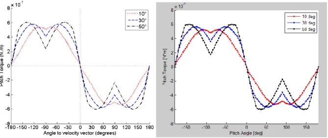
Figure 9.3 - Pitch Torque Model from [25] ... 76
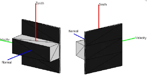
Figure 9.4 - RTM Geometric Model for Pitch Test Validation ... 76
Figure 9.5 - Pitch Test Validation ... 77
Figure 9.6 - MotherCube RTM Model ... 78
Figure 9.7 - Aerodynamic Drag (RTM Result) ... 78
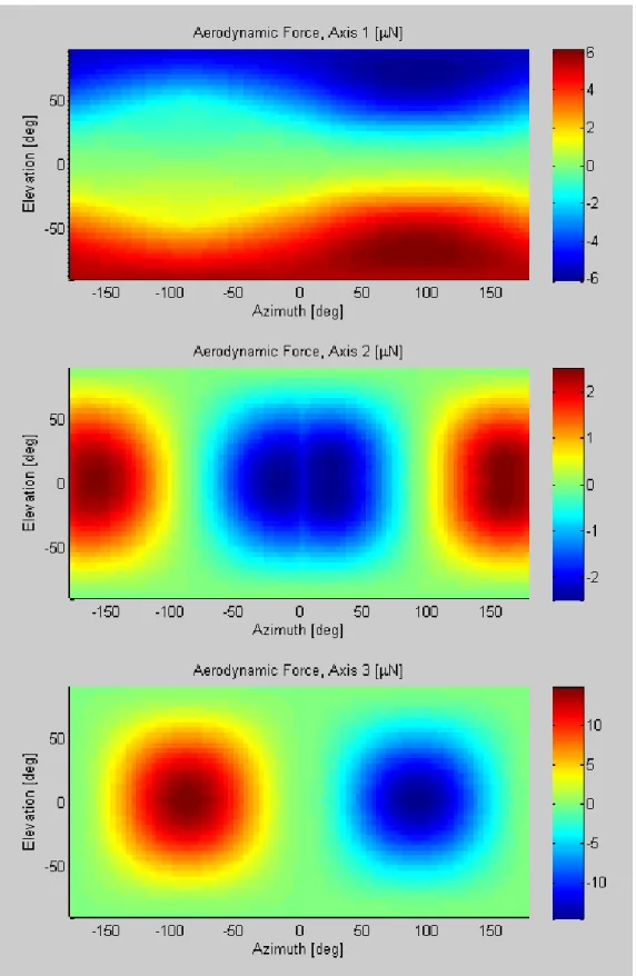
Figure 9.8 - Aerodynamic Forces (RTM Result) ... 79
Figure 9.9 - Aerodynamic Torques (RTM Result) ... 80
Figure 9.10 - Solar Forces (RTM Result) ... 81
Figure 9.11 - Solar Torques (RTM Result) ... 82
Figure 9.12 - Solar Power (RTM Result) ... 83
Figure 10.1 - Average Atmospheric Density vs. Altitude (Modeled) ... 87
Figure 10.2 - Magnetic Field Vectors at 500km Orbital Radius ... 88
Figure 11.1 - Sun Synchronous Orbit (ECI Frame) ... 90
Figure 11.2 - Case 1 State Response ... 92
10
Figure 11.4 - Case 1 Torques ... 94
Figure 11.5 - Case 2 Angular Rate Behavior ... 96
Figure 11.6 - Case 2 Angular State and Error... 97
Figure 11.7 - Case 2 State History ... 99
Figure 11.8 - Case 3 Velocity State History ... 100
Figure 11.9 - Case 3 Relative Force History ... 101
Figure 11.10 - Case 3 Weighted Error ... 102
Figure 11.11 - Case 3 Delta V ... 102
Figure 11.12 - Case 4 Position Relative Position State History ... 104
Figure 11.13 - Case 4 Velocity State History ... 105
Figure 11.14 - Relative Force Plot ... 106
Figure 11.15 - Relative Force Plot Zoomed In ... 107
Figure 11.16 - Case 4 Body Frame Force Commands after Local Allocation ... 108
Figure 11.17 - Case 4 Weighted Formation Error ... 109
11
L
IST OF
T
ABLES
Table 3.1 - List of Coordinate Frame Superscripts ... 24
Table 4.1 - Thruster Geometry ... 31
Table 4.2 - Body Axis Electrospray Thruster Force and Torque Limits... 33
Table 4.3 - Body Axis Magnetic Torque Coil Torque Limits ... 34
12
CHAPTER 1
I
NTRODUCTION
1.1 M
OTIVATION
A distributed satellite system (DSS) is defined as a set of spacecraft which are physically separated but which form part of a bigger system which derives functionality from the contributions of each member. There are two types of distributed satellite systems: constellations and formations. A ‘formation’ (or ‘cluster’) is characterized by utilizing control laws which couple the states of the member satellites to achieve the desired behavior. Constellations, on the other hand, may be designed so that their orbits complement the other members, but they are controlled relative to their own pre-defined reference trajectories rather than dynamically based on the behavior of the other members. Historically, constellations have been where one spacecraft is incapable of accomplishing the mission. The best example of a spacecraft constellation is the Global Positioning System (GPS), which uses multiple broadcasting satellites in a variety of orbits so that users can triangulate their position from the time of flight of the broadcast signals. Constellations have also been used to ensure high-availability, global communication (Iridium) or for coordinated remote sensing (‘A-Train’).
Spacecraft formations, on the other hand, typically seek to replace monolithic spacecraft with a set of smaller spacecraft. This ‘fractionation’ is expected to improve some of the following categories:
Flexibility – Because the members of a spacecraft formation are not physically connected,
the possibility of fast, dynamic reconfiguration allows a single set of hardware to be designed and used for a wide variety of tasks, albeit at a complexity cost [1].
Robustness – A system with many elements is often capable of complete or partial
functionality in the case of single element failure. Having a distributed architecture also means that partial upgrade or replacement of an in-place system is possible without needing to replace the entire system all at once.
Cost-effectiveness – One of the inherent benefits of an architecture composed of smaller
13
less costly than making one monolith [2]. Additionally, the flexibility and robustness benefits often also manifest themselves as a cost savings by reducing the requirements for hardware redundancy because the consequence of a single failure is much less severe. It also allows for reuse of common system elements.
DARPA’s System F6 concept [3] is an embodiment of these first three benefits of using a formation flying system. Its objective is to demonstrate the fractionation of individual subsystem functions within individual spacecraft which fly in formation and communicate wirelessly within the formation. For instance, there would be one spacecraft dedicated to ground communication, one to power, one for the payload operations, and so on.
Figure 1.1 - Artist's Depictions of DARPA’s System F6 [3]
The other benefit which can be leveraged from a formation flight mission is for payload performance:
Performance – There are several types of spacecraft payloads which benefit from having a
long baseline between sensors. Interferometers (often used for astronomy) are one striking example, where using elements separated by a long baseline can yield results equivalent to a filled aperture much larger than what could be physically realized in a space system. The now-cancelled Terrestrial Planet Finder (TPF) mission [4] is the embodiment of why a formation would be chosen for its enhanced performance. During its design, the TPF team was investigating two separate concepts for the mission to perform spectroscopy on exoplanets. The
14
first design was a traditional single-aperture monolith, which would have been on the order of 10m in diameters.
Figure 1.2 - Artist's Rendition of the Terrestrial Planet Finder Mission [5]
The second concept called for four 3.5m diameter apertures flying approximately 1000m in separation. Thus, a much smaller system would be as capable (or perhaps more so) than a monolith.
More recently, the PRISMA mission [6] was launched to demonstrate chemical-based propulsion for microsatellites as well as formation flight, homing, and rendezvous. The formation has two agents, only one of which has translational control.
Of course, using a formation flight architecture also poses some challenges. These challenges include the transfer of information (and potentially power or mass) and for the determination and control of the relative positions. These challenges are augmented by additional mission-specific hardware or operational constraints. This thesis will address the issues surrounding the control of the attitude and relative positions of a formation of Cubesats.
1.2 M
OTHER
C
UBE
M
ISSION
O
VERVIEW
Although most of the ideas contained in this thesis are generalizable, the need for most of them originated from a requirement or difficulty in designing the Attitude Determination and Control System (ADCS) for the MotherCube mission. Additionally, all of the numerical results are presented
15
using parameters from this mission. A brief description is given to familiarize the reader with some of the mission-specific objectives and challenges.
1.2.1 Mission Objectives (Relevant to ADCS)
1.2.1.1 Payload Objective: Radio Geolocation
The primary objective of the MotherCube (also called DSS) mission is to identify the location of radio sources by using three formation-flying satellites with receiver antennas to triangulate its position. On this mission, the radio sources will be VHF sources located on Earth, so the term ‘geolocation’ is often used to describe the payload objective. The mission also aims to demonstrate the on-orbit behavior of electrospray thrusters and satellite formation flight.
1.2.1.2 Demonstrate: Electrospray Thrusters
Electrospray thrusters (a type of colloid thrusters) are a form of electric propulsion [7]. The thrust is produced by electrostatic acceleration of microscopic charged droplets. These systems have several advantages over traditional (chemical) propulsion, which are:
High Specific Impulse – Electrically accelerating the fuel allows a much higher exhaust velocity than can be achieved using chemical propellants and gas nozzles. Specific impulses in the range of 1000 – 5000 seconds may be obtainable in a fully-developed system.
Precision Control – The thrust can be controlled to very high precision by varying both the voltage level and the length of the pulse. Most chemical systems have a much coarser level of control due to the ‘minimum impulse bit’, which is typically driven by the plumbing of the chemical system.
Scalability – the fundamental unit is a conical emitter tip, which has a diameter on the order of hundreds of micrometers. The thrusters are simply arrays made of thousands of emitter tips. This makes electrospray thrusters uniquely suited to propulsion for small satellites, as the arrays can easily be scaled to fit the smaller form factor where chemical systems become significantly less efficient.
Simple Plumbing – Electrospray thrusters do not require any moving parts, valves, or pressurized tanks. The fuel is drawn into the thruster via a porous substrate and operates in response to an applied voltage command.
16
Electric Energy – Unlike chemical propellant where the energy used to accelerate the reaction mass is derived from the chemical potential of the combustion reaction, electric propulsion requires an external energy source.
Complicated Power System – Electrospray systems require power at very high voltage (>1000 V) and low current ( < 1 mA), which requires special electronics to convert and regulate the power.
Low Thrust – The consequence of the aforementioned energy and electronics requirements
generally restrict feasible systems to thrust levels which are many orders of magnitude smaller than chemical systems. This significantly affects the types of trajectories and maneuvers which may be utilized, as impulsive maneuvers have lower delta V than low thrust maneuvers.
1.2.1.3 Demonstrate: Formation Flight
A spacecraft “formation” (or “cluster”) is defined as a group of spacecraft operating in close proximity such that control of their relative position is important. This differs from a “constellation” of satellites (such as the GPS satellites) which work together to achieve a common goal but do not actively control their distance from the other satellites in the constellation. Spacecraft formation flight is an important technology required for next-generation space telescopes, such as Terrestrial Planet Finder.
1.2.2 Basic Satellite Hardware Configuration
For this report, the dusk-dawn sun synchronous concept is assumed. At the time of writing, this concept is considered more likely and preferable and it matches the analysis performed thus far. It is possible that the hardware configuration could change if a different orbit is utilized.
The primary components of the MotherCube hardware are: 1. Electrospray Thrusters
2. Solar Panels 3. GPS Antenna
4. Patch Antenna (for ground communication) 5. Payload Antenna
17
7. Magnetic Torque Coils (around the edges of the bus frame and the solar panels)
Figure 1.3 - MotherCube Hardware Configuration
1.3 T
HESIS
O
VERVIEW
The ultimate goal of the ADCS software design is to craft a set of algorithms which, when implemented onboard the spacecraft, produce the desired behavior. However, in order to evaluate such algorithms, a computer simulation is used to virtually replicate the space environment and its interaction with the spacecraft’s actuators and sensors.
18
Figure 1.4 - High Level Simulation Diagram
This thesis is divided into 12 chapters. Each chapter is essentially one or two of the blocks as shown in Figure 1.4. Chapter 2 provides a literature review and a gap analysis. Chapter 3 discusses the variety of coordinate frames and other conventions which are used throughout the thesis. Chapter 4 derives the model of the spacecraft’s physical properties, actuators, and sensors. Chapter 5 derives the control law for relative formation positional control and the formation allocator which assigns control actions to individual spacecraft in the formation. Chapter 6 presents two control laws for regulating the attitude and attitude rate of the spacecraft. Chapter 7 presents the local allocator (or ‘mixer’) function which assigns actuator commands based on a set of desired forces and torques. Chapter 8 discusses the estimation of the system state and presents an estimator. Chapter 9 derives an intermediate-accuracy ray-tracing method for computing attitude-dependent forces and torques resulting from aerodynamic or solar effects. Chapter 10 presents an overview of
19
the simulation effort, including a look at the environmental models which are inputs to the simulation. Chapter 11 presents the simulation results for four use cases. Finally, Chapter 12 concludes the thesis with a summary and recommendations for future work.
20
CHAPTER 2
L
ITERATURE
R
EVIEW
2.1 L
ITERATURE
R
EVIEW
In the last decade, a great deal of research on the guidance, navigation, and control of spacecraft formation flight missions has emerged due to its identification as a critical technology along the path to many NASA objectives (such as exoplanet detection and characterization [4], synthetic aperture radar [8], and gravitational mapping [9]). This section will discuss some of the relevant literature in the control of formations, which is defined as the generation of control actions to achieve the desired system behavior.
A dedicated two-part survey of formation flight guidance [10] and control [11] by gives an excellent overview of the major types of formation flight control along with numerous references to examples of each. This survey broadly groups formation flight control methodologies into two dynamical regimes. The dynamics can be broadly grouped as:
Deep Space (DS) – This is defined to be a region of space where spacecraft translational
dynamics are well approximated by a double integrator model.
Planetary Orbital Environment (POE) – Significant environmental disturbances such as
gravity or aerodynamic drag affect spacecraft motion.
The survey further divides the types of control into five categories, unrelated to the dynamic environment:
Multi-Input, Multi-Output (MIMO) – In this architecture, the dynamics for the entire
formation are treated as one large MIMO system and modern methods of control are directly applied. The primary benefit of this architecture is its optimality and stability, which are due to the fact that the full state of the entire formation is available. However, the primary downside is high communication requirements and problems with scalability for large formations. The MIMO formulation is not robust with respect to changes in formation size, because the full state is used in the control design.
21
Leader/Follower (L/F) – Also called Chief/Deputy, this is the most studied type of
formation control because it simplifies the control of an entire formation into individual tracking problems by selecting a strict hierarchy whereby Follower satellites control their position relative to a designated Leader(s). The most common architecture is the single-layer L/F, where all spacecraft follow the same leader. Another common L/F architecture is the chain, where each spacecraft follows the preceding one. An important feature of this architecture is the relationship between any two spacecraft MUST be either leader, follower, or unrelated. The primary benefit to this architecture is its robustness to changes in formation. Adding a new member does not affect any of the existing members because the new member will be a Follower. In the event of the failure of a leader, only its followers are affected and they can be reassigned to new leaders. The one major downside to this architecture is that it is not globally optimal.
Virtual Structure (VS) – The objective of this method of formation control is to produce
formation behavior which mimics the behavior of objects embedded in a rigid structure such as a truss. The most well-known example of this type of controller is the Terrestrial Planet Finder mission [4].
Cyclic – A cyclic controller is similar to a L/F architecture but without the hierarchal
constraint. In this way, two spacecraft can both feedback on their relative state. Many formulations of cyclic control lend themselves to decentralized control by creating relationships among the nearest neighbors in a formation.
Behavioral – A behavioral controller combines the output of multiple controllers designed
for different behaviors, where formation control is considered a mandatory behavior. For instance, a L/F architecture could be combined with a collision avoidance algorithm. Rather than a standalone architecture, the behavioral control methodology is an augmentation of one or more of the other control methodologies.
In addition to these five categories, a recent special focus has been centered around ‘formation initialization’ [12] [13], which seeks to analytically or numerically identify collision- or drift-free trajectories based only on the initial conditions [14]. This strategy typically results in one or many open loop maneuvers which produce acceptable behavior for some time period, at which point the formation is reinitialized. The assumption is typically that impulsive thrust is used to enforce the initialization condition, so it is not suitable for electric propulsion.
22
2.2 G
AP
A
NALYSIS
One significant limitation in the utility of much of the formation flight literature is that it assumes unconstrained thrust direction while neglecting attitude dynamics. For large systems with impulsive thrust, this is perhaps well justified, as a single-thruster spacecraft could rotate to the desired attitude between maneuvers. However, for electrically propelled formations or for small satellite formations with significant hardware limitations due to size, this is a significant limitation. Some limited work has been done in this area to demonstrate closed periodic trajectories using a single unilateral thruster with passive magnetic stabilization [15] [16].
This thesis seeks to address this limitation – the conversion of desired relative accelerations (between spacecraft) to actuator commands for body-fixed thrusters with saturation constraints. An extension of this allows for the interaction with other spacecraft attitude actuators to simultaneously control the spacecraft attitude according to an independent attitude control law.
23
CHAPTER 3
C
OORDINATE
S
YSTEMS AND
N
OTATION
3.1 U
NITS
All quantities are expressed in metric units. Specifically, the MKS notation is used, which means that distances are expressed in meters, mass is expressed in kilograms, and time is expressed in seconds. All angles are expressed in radians and all coordinate frames are assumed to be right-handed.
3.2 N
OTATION
Vector quantities are denoted with bold type. is a vector, is not a vector.
Accent characters are used with specific meaning throughout the thesis. These uses are:
True Value ̅̅̅̅ Measured Value ̂ Unit Vector ̂ Estimated Value ̃ Modeled Value
̇ Time Derivative of Value
3.3 Q
UATERNION
C
ONVENTIONS
The default attitude representation used in this report is quaternions because they are computationally faster and have lower storage requirements. This thesis does not give a full overview of quaternion math. This can be found in [17] and [18]. However, the most notable elements will be repeated here for clarity. The most important item is that the quaternions used here have the scalar element fourth.
24
[ ] (3.1)
Additionally, because quaternions have a sign ambiguity, the additional constraint of is imposed. If at any point, q4 becomes negative, then the entire quaternion undergoes a sign change, which preserves the physical meaning of the quaternion. Finally, the notation used in this thesis for the skew matrix is as follows:
[
] (3.2)
3.4 C
OORDINATE
F
RAME
N
OTATION AND
C
ONVENTIONS
This section describes the notations which will be used for all vector quantities which are expressed in a particular coordinate frame. A single superscript is used to denote the frame in which a vector quantity appears. The following table is a complete list of all coordinate frames and their superscript designations:
Table 3.1 - List of Coordinate Frame Superscripts
Inertial (ECI)
Body
ECEF
NED
LVLH
Ray Tracing Body
For quantities which describe the relationship between two coordinate frames, the superscript is expressed in the ‘to-from’ notation. Direction cosine matrices (also called ‘rotation matrices’) are typically denoted by a capital ‘R’ and quaternions are denoted by a lowercase ‘q’. Thus, quantities are related in the following way:
25
(3.3)
is a vector expressed in the body frame, is the same quantity expressed in the inertial frame, and is the DCM which relates the two frames. This notation is very intuitive, because equations
which appropriately transform the quantities must match adjacent superscripts.
3.5 E
ARTH
-C
ENTERED
I
NERTIAL
(ECI)
The inertial (also called ‘global’ or ‘fixed’) is referenced to the J2000 ECI reference frame. It is defined as the Earth's Mean Equator and Equinox at 12:00 Terrestrial Time on 1 January 2000. The X-axis is aligned with the mean equinox. The Z-axis is aligned with the Earth's spin axis or celestial North Pole. The Y-axis is rotated by 90° East about the celestial equator. This system is shown in Figure 3.1.
Figure 3.1 - Inertial Coordinate System [Image: Wikimedia]
3.6 E
ARTH
-C
ENTERED
,
E
ARTH
-F
IXED
(ECEF)
ECEF coordinates are very similar to ECI coordinates except that the reference frame rotates with the Earth such that the axis intersects the sphere of the Earth at 0° latitude and 0° longitude, the axis is aligned with the earth’s spin axis and the axis completes the right handle system. The rotation matrix which relates positions in ECEF and ECI is:
26
[ ] (3.4)
(3.5)
Where is the fractional number of days since noon on January 1, 2000.
3.7 N
ORTH
-E
AST
-D
OWN
(NED)
Also known as geodetic coordinates, this coordinate system is parameterized by latitude (ϕ), longitude (λ) and height or altitude (h). The conversion from these parameters to ECEF coordinates is straightforward: [ ] [ ] (3.6)
Conversion from NED to ECEF is much less straightforward. One approximation [18] which is valid for heights below 1000 km is:
( ̅ ) (3.7) (3.8) (3.9) √ (3.10) √ (3.11)
27
̅ (3.12)
(
) (3.13)
The parameters used to describe the geoid are: . Note that N is the Earth’s radius at a given latitude.
The rotation matrix which relates the ECEF coordinate frame and the NED coordinate frame is:
[
] (3.14)
3.8 L
OCAL
-V
ERTICAL
,
L
OCAL
-H
ORIZONTAL
(LVLH)
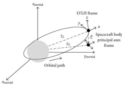
The most-used coordinate frame in this work is the Local-Vertical Local-Horizontal coordinate frame. This frame rotates with the chief orbit and is always aligned such that the x-direction is in the local vertical (‘radial’), the z-direction is in the direction of the orbit normal, and the y-direction forms a right-handed coordinate system. The origin of the system is at the center of mass of the chief. In this work, it is assumed that all orbits are circular, which means that the y-direction is always in the velocity direction (also called ‘tangential’ or ‘alongtrack’ direction). This system is shown in Figure 3.2.
28
Figure 3.2 - LVLH Coordinate System
The rotation matrix between the LVLH frame and the inertial frame can be computed from the inertial position and velocity vectors of the chief as follows:
̂ ‖ ‖ (3.15) ̂ ‖ ‖ (3.16) ̂ ̂ ̂ (3.17) [ ̂ ̂ ̂ ] (3.18)
To be very clear, the position of a spacecraft in the LVLH frame can be written in the following ways:
̂ ̂ ̂ (3.19)
It is worth noting that all of the deputy spacecraft use the same LVLH coordinate frame – relative to the chief. This transformation changes as the chief moves through the orbit. Because the chief’s state is not always known to the deputies, it is often the case that the transformation between
29
inertial and LVLH coordinates is computed using the deputy’s inertial states instead of the chief’s, introducing some error.
3.9 B
ODY
C
OORDINATE
S
YSTEM
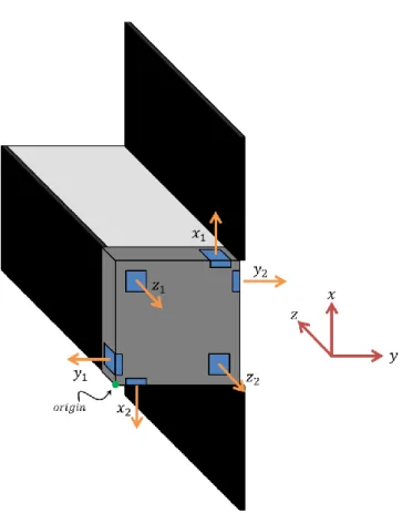
The body coordinate system is defined such that the GPS antenna is on the +X face of the main bus body, the solar panels are the on the +Y face, and the electrospray thruster slice is located on the –Z face. The origin is on the located at the (-X, -Y, -Z) corner of the thruster slice.
Figure 3.3 - Body Coordinate System during Nominal Mission
In the nominal configuration, the +X body axis is aligned with the +x LVLH axis, the +Y body axis is aligned with the –z LVLH axis, and the +Z body axis is aligned with the +y LVLH axis. Thus the nominal relation between the body and LVLH frames is given by:
[
30
CHAPTER 4
S
PACECRAFT
M
ODEL
4.1 P
HYSICAL
P
ROPERTIES
The spacecraft are 3U Cubesats, which means the mass is limited to 4kg and the envelope dimensions are 10cm-by-10cm-by-34cm. The spacecraft can essentially be considered to come in two pieces: the solar panels and the spacecraft bus. A 3U-by-3U solar panel is attached to the +Y face of the spacecraft and a 3U-by-1U solar panel is attached to the –Y face of the spacecraft. The solar panels are assumed to have an areal density of 0.5 g/cm2, yielding a total solar panel mass of
600g. Due to the center of mass requirements, it is assumed that mass balancing will be used to bring the spacecraft center of mass to the geometric center of the spacecraft bus. Because the internal configuration of the spacecraft is still unknown, the remainder of the mass will be assumed to be evenly distributed in the spacecraft bus. Thus, the inertia tensor taken at the spacecraft center of mass can be approximated as:
[
] (4.1)
The center of mass is assumed to be located at the geometric center.
(4.2)
4.2 E
LECTROSPRAY
T
HRUSTERS
31
4.2.1 Geometry
Figure 4.1 - Electrospray Thruster Configuration
The thrusters are assumed to produce a point force located at their center. The thrust vector is assumed to be normal to the thruster slice. These properties are tabulated in:
Table 4.1 - Thruster Geometry
Thruster Index Location [cm] Thrust Direction
1 2 3 4 5 6
It should be noted that the force produced by each thruster is in the opposite direction from its thrust vector. The moment arm for the i'th thruster is defined as:
32
(4.3)
Thus, the force and torque produced by the i'th thruster can be given by:
(4.4)
(4.5)
With being the thrust produced by the i'th thruster.
4.2.2 Thrust Modeling
As mentioned in Section 1.2.1.2, one of the main benefits of the electrospray thruster technology is that it can be precisely controlled by varying the input voltage and duty cycles - much more finely than possible using a pulsed chemical system. For this reason, it is assumed that any thrust level up to the thruster saturation limit can be commanded. It is also (obviously) the case that the thrusters cannot produce negative thrust. Thus, the constraints on each thruster can be expressed as:
(4.6)
The electronics required for power conversion and control place some limitations on the thrust levels which can be produced. It is out of scope to discuss the details of the electronics design and why these limitations exist, but the result on the thruster is that there is a limit on the total thrust which can be produced by the system at any one time.
∑
(4.7)
For this hardware configuration, each thruster can produce a maximum of 50 μN and the total thrust output is limited to 100 μN. Due to the hardware configuration, this yields the following limiting values assuming maximum control effort and an ideal center of mass:
33
Table 4.2 - Body Axis Electrospray Thruster Force and Torque Limits
Body Axis Thruster Force Limits [μN] Thruster Torque Limits [μNm]
-50 to +50 -8.5 to +8.5
-50 to +50 -8.5 to +8.5
0 to +100 -3.5 to 3.5
However, it should be noted that forces and torques about the and axes cannot be produced without generating disturbance forces and/or torques about the other axes. However, forces and torques about the axis can be produced independently and without introducing other disturbance torques.
4.3 T
ORQUE
C
OILS
The spacecraft is also equipped with magnetic torque coils (abbreviated MTQ) for attitude actuation. Magnetic torque coils function via the Lorentz force, which is the force which acts on moving charges in an electric field. For a straight wire, the force can be expressed as:
(4.8)
Where F is the force [N], I is the current in the wire [A], Bm is the magnetic field vector [T], and l is
the wire vector [m], containing the magnitude and direction of the wire. If the wire is instead formed as a closed coil, the net force is zero but a torque is produced. Specifically:
(4.9)
Where is the number of turns of wire, is the cross-sectional area of the coil [m2],
has a magnitude proportional to the current in a single wire and a direction which aligns with the normal vector of the coil. is known as the dipole moment of an MTQ, and units of Am2.
There are three sets of torque coils – one mounted in line with each of the spacecraft body axes. The dipole moment can be varied simply be increasing or decreasing the current through the coils. Thus, the dipole moment can effectively be slewed to any direction at very high rate. Each coil is assumed to be separately controllable up to its maximum thrust. The maximum current in this case is determined by thermal concerns related to the wiring of the coils themselves. In order to prevent
34
overheating and possible damage, the current must be limited. Thus, each axis of the torque coil is limited as follow:
(4.10)
The preliminary mission study indicated that torque coils with a maximum dipole moment of 0.42 Am2 would be sufficient to overcome the expected disturbances. Because the final design is not yet
known, this is assumed to be the maximum dipole moment of the coil set around each axis. It should be noted that the torque coils must be unpowered when the magnetometer is taking data to prevent interference, so the actual coils will be sized such that their time-averaged maximum dipole moment includes this unpowered time.
This yields the following maximum torque values (assuming averaged magnetic field strength):
Table 4.3 - Body Axis Magnetic Torque Coil Torque Limits
Body Axis Thruster Torque Limits [μNm]
-18.9 to +18.9 -18.9 to +18.9 -18.9 to +18.9
The major downside to magnetic torque coils is that torque cannot be produced around the magnetic field vector, which means only two degrees of freedom are instantaneously controllable.
4.4 R
ATE
G
YROS
The spacecraft will have tri-axial digital gyroscopes for sensing the spacecraft’s angular rate of its body frame with respect to the inertial frame. The sensor which is tentatively selected for this task is a component of the Analog Devices ADIS16488 [19].
35
Figure 4.2 - ADIS16488 Inertial Measurement Unit
4.4.1 Sensor Model
Because this mission expects a relatively stable temperature profile and does not anticipate high acceleration, the parameters which are most likely to affect the spacecraft estimation are the initial bias error, the in-run bias stability, and the angular random walk. The gyros are modeled as a first order Markov process with the following model:
̅ (4.11)
̇ (4.12)
(4.13)
Where is the gyro bias vector, is the initial bias error, and are zero-mean Gaussian
white-noise with spectral densities of , respectively.
4.4.2 Expected Use
The intended use of this sensor is to measure the spacecraft’s angular rate for attitude determination. Upon ejection from the P-POD, it is likely that the spacecraft may be spinning at a rate of up to 3 degrees per second. However, in the nominal case, the spacecraft will be rotating at a rate of once per orbit, or 0.06 degrees per second.
4.4.3 Derivation of Numerical Values
Unfortunately, the sensor specifications are not given in terms of white noise. Because this gyro is a “smart” gyro, the device samples the gyro much more frequently than the user sample rate and
36
performs some internal filtering to give a more accurate sensor measurement at the lower sample rate requested by the user to reduce the noise in the measurement. This is characterized by an Angular Random Walk parameter with units of degrees per √ . This can be converted to white noise if the user’s sampling time of the sensor is known by:
√
√
√ (4.14)
The white noise on the bias drift is computed from the in-run bias stability assuming that it can also be modeled as a random walk process and converted to a white noise process in a similar way. In this case, the sensor specification lists a standard deviation on the bias (units of degree/time). However, if it is assumed that this bound was derived by testing the performance for a finite time interval, it can be conservatively converted into an random walk process. Thus:
√ (4.15)
4.5 M
AGNETOMETER
The ADIS16488 also has a tri-axial magnetometer which measures the magnetic field in the body frame.
4.5.1 Sensor Model
The sensor imperfection which will affect the system most is the output sensor noise. The magnetometer output is modeled as:
̅ (4.16)
Where is a zero mean Guassian white noise process with a spectral density of .
4.5.2 Expected Use
The intended use of this sensor is to measure the Earth’s magnetic field for comparison with an onboard model for use in attitude determination. The Earth’s magnetic field varies in intensity from approximately 30-60 μT. Because the magnetic field varies significantly over the orbit, the magnetic field may be oriented in any direction with respect to the body, even during nominal operations.
37
4.5.3 Derivation of Numerical Values
However, the output noise is specified as a noise density which can be converted to a white noise standard deviation as:
√
√
√ (4.17)
The amount of error introduced in this way is similar to the least significant bit, which is 10 nT, and represent an error of approximately 0.03% of the expected magnetic field.
4.6 S
UN
S
ENSORS
The sun sensors to be used on the spacecraft are the Space Micro Medium Sun Sensor [20]. These sun sensors are capable of measuring the direction to the sun in the body frame. However, the sensors can only determine two degrees of freedom, as the degree of freedom around the sun vector is not measurable. The spacecraft is expected to have two of these sensors, one centered on the face and pointing along the axis. The other will be centered on the face and pointing along the axis.
Figure 4.3 - Space Micro Coarse Sun Sensor
4.6.1 Sensor Model
Because the sun sensor only measures the direction of the sun, it can be modeled as a unit vector. Its error can be modeled by rotating the true sun vector. For small angles, this can be approximated as: ̅ [ ] (4.18)
38
Where is the unit vector pointing in the direction of the sun, expressed in the body frame. ,
, and are independent zero-mean white noise processes with a variance of .
In order for a valid measurement to be made, the sun must be in the field of view of the sensor. Most sensors have cone-shaped baffles, so a simple check for sensor validity is:
(4.19)
Where is the direction vector of the sun sensor and is the half-cone angle of the field of
view of the sensor.
4.6.2 Expected Use
The intended use of the sun sensor is to measure the direction of the sun for comparison with an onboard model for use in attitude determination. In nominal operations, the sun sensors on the face should have a continuous view of the sun. If the attitude is off-nominal, it is possible that none of the sun sensors will be able to see the sun.
4.6.3 Derivation of Numerical Values
The sensor’s data sheet gives centroid error values for the entire field of view of the sensor. The majority of the field of view has an error less than 1°, so the sensor’s angular standard deviation is conservatively assumed to have .
39
CHAPTER 5
F
ORMATION
C
ONTROL
D
ESIGN
5.1 O
RBITAL
S
TATE
E
QUATIONS
The starting point for the control design is the Hill-Clohessy-Wiltshire (HCW) equations for relative orbital motion [21]. These are a linearized set of equations for the motion of a member of the formation (a ‘deputy’) relative to an imaginary, uncontrolled object in a perfectly circular orbit (the ‘chief’). The equations for a single satellite are given below (all quantities in LVLH coordinates):
̈ ̇ (5.1)
̈ ̇ (5.2)
̈ (5.3)
Where ux, uy, and uz are external accelerations in the LVLH x, y, and z directions, respectively. ω (not
to be confused with the angular rate vector ω) is the angular rate of the chief’s orbit, and can be calculated as:
√ (5.4)
Where μE is the gravitational constant of the Earth, and a is the semi-major axis of the reference
orbit. Rewriting these equations in matrix form yields:
̇ (5.5)
40 [ ] [ ] [ ̇ ̇ ̇] [ ] (5.6)
However, because the forces are produced by thrusters fixed to the spacecraft body, it is more useful to describe the control vector in terms of the body axes, since the body z-axis thruster is the only one which can fire without creating disturbance torques. This is important to distinguish so that this control can be weighted later. This changes the equations to:
̇ (5.7)
[ ] [ ] (5.8)
For expressing the full state of the system, the states of each satellite are simply concatenated to form another equation of the form:
̇ ̅ ̅ (5.9) ̅ [ ] ̅ [ ] [ ] [ ] (5.10)
Because all the satellites are referenced to the same circular orbit, .
In the HCW formulation, it is possible to achieve Passive Relative Orbits (PROs) if certain relationships are held between states. In these orbits, the satellites will oscillate periodically about a center, which will not drift over time. These types of orbits are the foundation for fuel-efficient formation flight. In general, randomly selected conditions will not yield PROs. The condition which yields a PRO with a common center is the following (note that string of pearls does NOT obey this):
41
The characteristic shape shared by all PRO’s is a 1:2 ellipse projected in the x-y plane. Because the z-direction is decoupled in the HCW formulation, the normal-direction motion of the satellite is not constrained by the PRO condition.
5.2 R
ELATIVE
S
TATE
E
QUATIONS
Because the electrospray thrusters cannot create thrust in the –z body direction, it is not possible to directly use continuous control methods and directly command all three spacecraft relative to the same fixed orbit. However, because the primary concern for mission success is relative positioning, the center of the cluster is actually not important. Therefore, the system state can be defined relative to one of the actual spacecraft instead of to an imaginary, uncontrolled spacecraft. Thus, the chief is now a controllable spacecraft instead of an imaginary point. This allows the size of system positional state vector to be reduced by six. The relative state vector is therefore defined as the state of spacecraft 2 and 3 relative to spacecraft 1. Thus the relative states and controls can be defined as:
(5.12)
These states have dynamics
̇ (5.13) [ ] [ ] [ ] [ ] (5.14)
5.3 C
LUSTER
C
ONTROL
L
AW
5.3.1 Relative Acceleration Command Generation
Because the system uses differential GPS, it will have relative position and velocity known to high accuracy. Therefore, it is appropriate to assume the full relative state is available and to use linear full-state feedback techniques for the control design.
Having created the relative state matrices as described in the previous section, the controller design is quite straightforward. The controller used is an infinite-horizon continuous linear-quadratic regulator (LQR). This controller minimizes the following error:
42
∫ (5.15)
The feedback control law which minimizes this cost is given by:
(5.16)
(5.17)
is found by solving the continuous time algebraic Ricatti equation:
(5.18)
This can be generated using the standard MATLAB function ‘lqr’ with the following simple syntax:
( ) (5.19)
are the weighting matrices on state error and control effort, respectively. Because
the system dynamics couple the position and velocity through the characteristic orbital rate, small velocity errors will eventually propagate into much larger position errors. Therefore, the state weighting matrix is chosen to more heavily penalize errors in velocity. Thus:
[
] [
] (5.20)
The final tuning parameter is the control weighting matrix, RLQR. Because the desired control action
is expressed as a relative acceleration in the LVLH frame (independent of the orientation of the spacecraft bodies), it is not desirable to penalize any axis of control more heavily. Thus, the control weighting matrix is:
[
] (5.21)
Thus, the tuning of the controller can be largely accomplished by varying the scalar value of ρ. It is always a good idea in beginning a control design to relate the parameters of the controller to parameters of the system. In this case, it was decided that a position error of 1km should yield
43
maximum control effort in the axial thruster. This yields a value of ρ =1014. Subsequent tuning
reveals that ρ values in the range of 1014 to 1016 are typically appropriate for most maneuvers.
To prevent saturation effects from causing drastically unwanted behavior, the entire relative acceleration vector is scaled down if the magnitude of any of its components exceed the maximum acceleration producible by the thrusters:
‖ ‖
{ ‖ ‖} (5.22)
5.3.2 Addition of a Reference Trajectory
Because full-state feedback is used, constant reference commands can be easily added:
(5.23)
The most common formation examined is the ‘string of pearls’ which is a constant separation in the velocity direction. The design reference trajectory for this mission is the 10km string of pearls configuration. This is represented as:
[ ] (5.24)
5.3.3 Allocation of Control to Individual Spacecraft
This control law generates a set of desired relative accelerations , expressed in the
LVLH frame of the chief. Because communication is assumed to be infrequent, it is desirable for centralized command generation to be infrequent. For the design reference mission, the spacecraft should all be nominally oriented and would therefore have a constant orientation in the LVLH frame. However, in the interest of having a more robust control design which can accommodate attitude control modes such as inertial pointing or ground station tracking, or continue to operate in case of attitude actuator failure, a variable LVLH attitude is considered.
In order to produce the control desired by the LQR controller, all three spacecraft must fire their thrusters such that the net relative acceleration is equal to the desired value. To accomplish this,
44
control is allocated to each satellite as a desired LVLH force which must be maintained until the next centralized control update. Each satellite must then calculate its own thruster firings based on its instantaneous attitude in order to produce that LVLH force (or as close as possible) at every control cycle.
However, because of the limitation that the spacecraft cannot produce any thrust in the direction, the control allocator must consider the spacecraft’s attitude to some extent in order to ensure that the allocated control is feasible based on its current attitude. Therefore, the assumption is made that the LVLH attitude is nearly constant between centralized control cycles (though possibly varying over longer timescales).
The method used for control allocation is constrained linear least squares optimization. The problem statement for this type of problem is:
‖ ‖ (5.25)
In this case, the optimization variables are the actuator forces:
[ ] (5.26)
From the previously discussed thruster models, the solution space for the thrust commands can be obtained:
(5.27)
The total thrust constraint imposed by the thrust slice electronics is expressed via linear system inequalities . Although each thruster can only fire in the positive direction, the spacecraft can have net body thrusts as positive or negative. Thus, the total thrust constraint can only be expressed in a linear system by considering all cases of positive and negative . thrust can only be in the positive direction. Each spacecraft is therefore constrained by:
45
[
] [ ] (5.28)
Thus, the constraint on the overall system is given by:
[
] [ ] (5.29)
The actuator models from the previous sections can be combined into a linear system as:
[ ] (5.30)
Because the objective is to ensure a target relative acceleration, it could easily be the case that a solution which exactly produces the required relative acceleration has two spacecraft producing thrusts which cancel each other out, thus wasting fuel. In order to minimize the total fuel use, this system is additionally augmented with a set of equations to penalize control effort. Thus:
[ ] [ ] (5.31)
In order to ensure that this fuel-minimization takes second priority to actually producing the desired relative accelerations, a weighting matrix comprised of only positive diagonal elements is applied to the optimization:
‖ ‖ (5.32)
With:
[
] (5.33)
This problem is solved using an active-set quadratic programming algorithm (MATLAB lsqlin function or using the method from [22]), yielding the optimized . =10-3 was used. Recall that
46
this is a set of body forces. In order for formation control to be achieved, the relative accelerations must be those specified by the LQR control law. In order to maintain these relative accelerations with a variable attitude between centralized control cycles, the body forces are rotated back to LVLH forces which must then be regulated by the individual spacecraft as its attitude changes. Thus, the output of the cluster controller to each spacecraft is a force specified in the LVLH frame it must maintain continuously for the duration of the central control cycle. The commanded force on the i'th spacecraft can then be obtained from the least-squares algorithm solution as:
(5.34)
Using this formulation of control allocation is appropriate because it explicitly accounts for the thruster saturations and will therefore only produce feasible solutions. However, the obvious downside of this method is that the control commands may not exactly produce the desired relative accelerations. An additional downside is that the solving the constrained linear least squares problem requires software libraries which can solve quadratic programs. This may be too computationally intensive for some formation flight missions.
5.4 C
URVILINEAR
M
ODIFICATION
5.4.1 Coordinate System
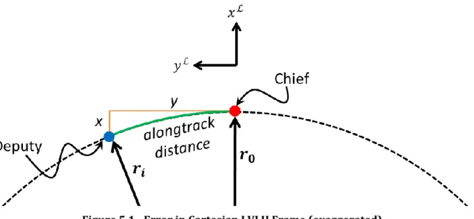
One of the major issues with the application of this control methodology is the conversion of the spacecraft’s actual state to the relative frame where the linearized equations hold. The HCW equations and formulation yield a rotating Cartesian coordinate system. Because the circular orbit is being approximated by a rectilinear coordinate system, the error introduced by the linear model increases with the distance from the chief. Note that in this section the ‘0’ subscript refers to the chief orbit and the ‘i' subscript refers to the i'th spacecraft. The chief, in this case, is one of the spacecraft.
47
Figure 5.1 - Error in Cartesian LVLH Frame (exaggerated)
For a spacecraft in a true string of pearls formation, this error has the effect of underestimating the alongtrack distance (an arclength) and introducing an error in the radial position. A similar image can be constructed for the out of plane error. This is because the string of pearls aims to emulate a differential true anomaly, which is an angular separation along a constant radius.
These types of errors can be reduced by switching to a curvilinear LVLH coordinate system, directly incorporating the fundamentally circular nature of orbits. The rotating system is established using two sequential rotations:
48
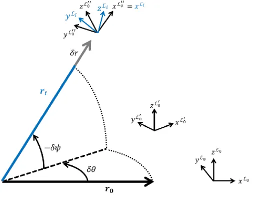
Figure 5.2 - Curvilinear Coordinate Diagram
The first rotation is by an angle counterclockwise about the ̂ axis, which is the orbit normal. This creates the intermediate frame. The second rotation is by an angle – about the ̂ axis which yields the coordinate system illustrated in Figure 5.2. This coordinate system represents
the curvilinear LVLH frame of the chief evaluated at the position of the deputy. The coordinate directions are given by the following equations:
̂ ̂ ̂ ̂ (5.35)
̂ ̂ ̂ (5.36)
̂ ̂ ̂ ̂ (5.37)
This can be more compactly represented by the rotation matrix which transforms the Cartesian coordinates expressed in the basis of evaluated at the location of the chief to the basis of evaluated at the location of the deputy:
[
49 The position vector can then be expressed as:
̂ [
] (5.39)
The other frame illustrated is the LVLH frame of the deputy itself, which is denoted as . Because the radial vector of the deputy’s LVLH frame is defined by the direction of its inertial position vector:
̂ ̂ (5.40)
However, the other two axes are not necessarily aligned.
5.4.2 Dynamics
The dynamics can be obtained by taking the time derivative of the deputy position vector in the curvilinear LVLH coordinates of the chief (which are time varying according to the motion of the chief) and equating that to the force of gravity plus the control accelerations. These equations are then linearized to obtain a new system. This derivation is performed in [23] for a slightly different coordinate system. However, the results are easily extended to this formulation with the following result:
̈ ̇ (5.41)
̈ ̇ (5.42)
̈ (5.43)
This system can be expressed as a standard linear system as follows:
(5.44) [ ] [ ] [ ̇ ̇ ̇] [ ] (5.45)
50
This yields the exciting result that this system is exactly the same as the HCW system previously used for control design! This means that curvilinear coordinates can be used without redoing the control design. The only change necessary is to redefine the transform from the global system state (ECI frame) to the LVLH frame using the new curvilinear relations. This has been implemented throughout the control design.
5.4.3 Converting from ECI to Curvilinear LVLH
Because this conversion only affects the cluster control calculation, it is reasonable to assume central knowledge of the all spacecraft ECI states (which is required for the cluster control calculations anyway). Note that this algorithm DOES allow for the chief to be in a non-circular orbit in order to obtain more accurate differential values. Note that this is by far the more important operation, because this is the direction the state representation takes at every control cycle in order to be controlled. The problem statement for this operation is as follows:
̇ ̇ ̇ (5.46)
The differential radius is trivially calculated as:
(5.47)
First, the position vector must be expressed in the chief’s Cartesian coordinates. The transformation matrix is obtained in the usual way for the Cartesian LVLH frame about the chief.
(5.48)
The differential out-of-plane angle can then be calculated as:
( ) (5.49)
The alongtrack angle can be computed in similar fashion:
(
51
The velocity is slightly more complicated due to the conversion from inertial to rotating reference frame. First, the inertial components must be expressed in the chief’s frame evaluated at the deputy’s position. This is accomplished by the following transformation:
̆ (5.51)
The unusual notation is because this is an inertial vector expressed in the coordinates of a rotating frame, which would be very confusing to express using the usual notation. The same transform is applied to the ECI velocity of the chief, but evaluating the coordinate frame at the origin:
̆ (5.52)
The differential radial component is trivially obtained by:
̇ ̆ (5.53)
̇ ̆ (5.54)
̇ ̇ ̇ (5.55)
The differential normal velocity can be quickly obtained because the normal velocity of the chief in its own LVLH frame is zero by definition. Therefore:
̇ ̆ (5.56)
The differential tangential velocity can be similarly expressed as:
̇ ̆ (5.57)
̇ ̆ (5.58)
̇ ̇ ̇ (5.59)
52
5.4.4 Converting from Curvilinear LVLH to ECI
In order to convert from curvilinear LVLH coordinates to ECI, a slightly different process must be used because of the information available. The problem statement for this operation is:
̇ ̇ ̇ (5.60)
The first step is to compute the radius:
(5.61)
The position expressed in the LVLH frame can then be easily computed as:
[
] (5.62)
The inertial position is easily computed as:
(5.63)
The inertial velocity expressed in the frame can be computed as:
̆ [
̇ ̇ ( ̇ ̇ )
̇
] (5.64)
̇ and ̇ are computed as in the previous section. Finally, the velocity must be rotated into the inertial frame.
̆ (5.65)
![Figure 1.1 - Artist's Depictions of DARPA’s System F6 [3]](https://thumb-eu.123doks.com/thumbv2/123doknet/14122933.467965/13.918.130.783.425.660/figure-artist-s-depictions-darpa-s-f.webp)

![Figure 9.3 - Pitch Torque Model from [26]](https://thumb-eu.123doks.com/thumbv2/123doknet/14122933.467965/76.918.189.736.239.519/figure-pitch-torque-model-from.webp)