Predicting partially observed processes on temporal networks by Dynamics-Aware Node Embeddings (DyANE)

HAL Id: hal-03214704

https://hal.archives-ouvertes.fr/hal-03214704

Submitted on 2 May 2021

HAL is a multi-disciplinary open access

archive for the deposit and dissemination of

sci-entific research documents, whether they are

pub-lished or not. The documents may come from

teaching and research institutions in France or

abroad, or from public or private research centers.

L’archive ouverte pluridisciplinaire HAL, est

destinée au dépôt et à la diffusion de documents

scientifiques de niveau recherche, publiés ou non,

émanant des établissements d’enseignement et de

recherche français ou étrangers, des laboratoires

publics ou privés.

(DyANE)

Koya Sato, Mizuki Oka, Alain Barrat, Ciro Cattuto

To cite this version:

Koya Sato, Mizuki Oka, Alain Barrat, Ciro Cattuto. Predicting partially observed processes on

tem-poral networks by Dynamics-Aware Node Embeddings (DyANE). EPJ Data Science, EDP Sciences,

2021, 10, pp.22. �10.1140/epjds/s13688-021-00277-8�. �hal-03214704�

REGULAR ARTICLE

Predicting partially observed processes on

temporal networks by Dynamics-Aware Node

Embeddings (DyANE)

Koya Sato

_{, Mizuki Oka}

_{, Alain Barrat}

_{and Ciro Cattuto}

*_{Correspondence:} alain.barrat@cpt.univ-mrs.fr 2_{Aix Marseille Univ, Universit´e de} Toulon, CNRS, CPT, Turing Center for Living Systems, Marseille, France

3_{Tokyo Institute of Technology,} Tokyo, Japan

Full list of author information is available at the end of the article

Abstract

Low-dimensional vector representations of network nodes have proven successful to feed graph data to machine learning algorithms and to improve performance across diverse tasks. Most of the embedding techniques, however, have been developed with the goal of achieving dense, low-dimensional encoding of network structure and patterns. Here, we present a node embedding technique aimed at providing low-dimensional feature vectors that are informative of dynamical processes occurring over temporal networks – rather than of the network structure itself – with the goal of enabling prediction tasks related to the evolution and outcome of these processes. We achieve this by using a lossless modified supra-adjacency representation of temporal networks and building on standard embedding techniques for static graphs based on random-walks. We show that the resulting embedding vectors are useful for prediction tasks related to paradigmatic dynamical processes, namely epidemic spreading over empirical temporal networks. In particular, we illustrate the performance of our approach for the prediction of nodes’ epidemic states in single instances of a spreading process. We show how framing this task as a supervised multi-label classification task on the embedding vectors allows us to estimate the temporal evolution of the entire system from a partial sampling of nodes at random times, with potential impact for nowcasting infectious disease dynamics.

Keywords: temporal networks; node embedding; dynamical processes

1 Introduction

The ubiquity of network representations of widely different systems has led to a flourishing of methods aimed at the analysis of their structure [1, 2] and of pro-cesses taking place on networks, such as information diffusion, epidemic spread, synchronization, etc [3, 4]. Recently, these investigations have been extended to the case of temporal networks, in which nodes and links can appear and disappear in time [5, 6].

Most works aim in particular at understanding how the network’s features impact the outcome of processes taking place on top of them, usually considering averages over many realizations of a stochastic process. A less considered issue concerns the reconstruction of partially observed processes taking place on a network. Indeed, given a dynamical process occurring on a network, such that nodes change state over time, in a realistic setting only partial knowledge of this evolution can in general be envisioned, as for instance in diffusion processes such as the spread of contagious

diseases or rumors. Recovering the complete information on the unfolding of the process from partial observations can then be of crucial importance, for instance to estimate the actual impact of a spread whose evolution is only partially known, and whose parameters are a priori unknown. This issue has been addressed in the specific case of spreading processes, under various hypothesis. For instance, some works have put forward methods to recover the state of all nodes and the seeds of a spread from a partial observation of nodes at a given time [7, 8], without attempting to recover the whole temporal evolution of the process. Methods to recover the state evolution of all nodes have also been proposed, using as input snapshots of the whole system, i.e., the knowledge of the state of all the nodes at a certain time [9–11]. Finally, several methods using partially observed snapshots have also been proposed [8, 12–14], typically based on strong assumptions on the nature of the underlying diffusion process.

Here, we propose a novel approach to tackle the general issue of recovering all the information about a single instance of a partially observed and unknown process taking place on a known temporal network, leveraging the recent development of node embedding methods. Network node embedding methods have indeed recently gained a lot of popularity [15–17] as tools able to explore network structure, and we propose here that embeddings can also be designed in order to recover infoma-tion on dynamical processes on networks. In short, a node embedding maps each node of a network into a low-dimensional vector, such that the vectors representing different nodes are close if the network nodes share some similarity or are close in the network. Node embeddings thus aim at exposing in the low-dimensional space structural features and relevant patterns of the network that are not necessarily ev-ident in the network representation. Most importantly, the embedding vectors can be used as feature vectors in machine learning applications, and have been shown to yield improved performance for tasks such as node classification, link prediction, clustering, or visualization [16].

Here we show that node embedding methods can also be tailored to the study of dynamical processes on temporal networks, and in particular to the task described above of predicting the evolution and outcome of any instance of the dynamics (e.g., an epidemic outbreak) from partial information and without detailed knowledge of the dynamical process itself. We notice on the other hand that the task at hand concerns a temporal network in discrete time on a finite interval, assumed to be fully known. A useful embedding should thus yield low-dimensional vectors that encode information relevant to the dynamics of the process occurring over a tem-poral network – rather than information about the network structure itself. Since dynamical processes unfold over time-respecting paths determined by the underly-ing network and by its evolution over time, we argue that the sought embeddunderly-ings should be informative of these paths – the paths along which information can prop-agate. Driven by this idea, we propose to first map the temporal network to a static graph representation without losing any temporal information. We note that this is in contrast with aggregated representations, in which the temporal information is lost [18], even if the aggregation procedure can be tailored to specific contexts such as epidemic processes on networks [19]. Higher-order aggregate networks, which take into account that not all the paths present in aggregated representations are

actually realizable, capture more temporal dependencies than usual aggregation, and processes simulated on such higher-order representations better reflect the true dynamics on the raw data [20–22]. For instance, such higher-order representations yield better estimations of centrality measures in temporal networks [21, 22]. Re-cently, two completely lossless static representations of temporal networks have moreover been put forward: the so-called supra-adjacency representation, whose nodes are the (node,time) pairs of the original temporal network [23], and the event-graph [24, 25], in which all temporal events are represented as nodes of a static graph. We propose here to modify the original supra-adjacency representa-tion method: we only consider nodes at those times when they interact, and we map the original temporal edges to edges between the corresponding (node,time) pairs: all nodes and temporal edges are represented, ensuring that no temporal informa-tion is lost. Crucially, this static graph representainforma-tion preserves all the temporal paths of the original temporal network (i.e., the paths supporting and constraining the dynamical process at hand), so that it does not suffer from the limitations of aggregated representations [20]. An example of the supra-adjacency representation we use here is shown in Fig. 1. Since the resulting representation is a static graph, we can then apply standard embedding techniques: we focus on embeddings based on random walks [26, 27] as they provide an efficient way to sample the relevant paths.

We show the performance of the proposed embeddings for the prediction of par-tially observed processes in the context of a paradigmatic dynamical process – epidemic spread over temporal networks – in which network nodes exist in few discrete states and the dynamics consists of transitions between such states (e.g., a “susceptible” node becoming “infectious”). As described above, we focus on the task of predicting the nodes’ states over time for a single realization of the epidemic process. Specifically, we set up a multi-label supervised classification problem with a training set obtained by sampling the node states at random times, with no in-formation about the mechanics of state transitions nor on the parameters of the epidemic process. In summary, our contributions are as follows:

• We propose a new method for node embedding tailored to the study of dynam-ical process on temporal networks, using a modified supra-adjacency repre-sentation for temporal networks and building on standard random-walk based embeddings for static graphs.

• We show that in the important case of epidemic spreading, a good predic-tion performance of nodes’ states can be achieved in a supervised multi-label classification setting informed by the proposed embeddings.

• We show that our method achieves good performance in estimating the tem-poral evolution of the entire system from sparse observations, consistently across several data sets and across a broad range of parameters of the epi-demic model. Our approach requires no fine-tuning of the embedding hyper-parameters and yields consistently superior performance with respect to other embedding methods.

The paper is organized as follows: we first formulate in detail the problem at hand in Section 2. We then describe our approach in Section 3 and show the results of numerical experiments in Section 4. We conclude with some perspectives in Section 5.

2 Problem Formulation

Let us first state in general terms the problem we want to address: given a known temporal network over a given time interval, an instance of an unknown process unfolding on this network and a partial observation of the dynamical states of the nodes, we want to recover the dynamical state of all nodes at all times of the temporal network. Crucially, this prediction must be performed without any information on the details of the dynamical process taking place on the network, except for the set of possible states of each node. In particular, we do not make any assumption on the type of transitions, the parameter values, nor even on the reversibility or irreversibility of the process. Moreover, this prediction does not concern an average over various realizations of the same process, but instead one single realization, which has been partially observed. Note that this task concerns a fully known temporal network, and the recovery of the nodes’ states over the time span of the temporal network: we do not consider a situation in which information on the temporal network and the state of the nodes would be arriving in real-time in a streaming fashion.

2.1 Temporal network

In more precise terms, we consider a temporal network g in discrete time on a time interval T = (1, 2, · · · , |T |), i.e., a set V of N = |V | nodes and a set of temporal edges of the form (i, j, t) denoting that nodes i and j are in interaction at time t ∈ T . Note that each temporal edge can also potentially carry a weight wij(t). The set of temporal edges at t is denoted Et, and Vt is the set of nodes which have at least one temporal edge at t: the snapshot network at t is the undirected weighted network Gt= (Vt, Et). We assume in the following that the whole temporal network is known.

For each node i, we define its set of active times Ti as the set of timestamps t in which it is involved in at least one temporal edge (i.e., such that i ∈ Vt). We denote the a-th active time of i by ti,a ∈ Ti, with ti,a < ti,a+1, and we define the set of active copies of each node i, that we call ”active nodes”, as Vi= {(i, t)|t ∈ Ti}. An active node is thus of the form (node,time). The overall set of active nodes is the union of all the sets of active nodes, i.e., V = ∪i∈VVi.

2.2 Dynamical process

We consider a dynamical process taking place on the weighted temporal network, such that each node i ∈ V can be at each time in one of a finite set of discrete states S. Nodes can change state either spontaneously or through interaction along tem-poral edges. Our definition is thus very general and encompasses a wide variety of processes on networks, such as models of epidemic propagation, rumor propagation, opinion formation or cascading processes [3, 28, 29].

While the problem description is very general, we will focus here on a paradigmatic dynamical process of strong relevance, namely the Susceptible-Infectious-Recovered (SIR) model for epidemic spreading, which is widely used to model contagious infections such as flu-like diseases [30]. In this model, each node can be at each time in one of three possible states: susceptible (S), infectious (I), and recovered (R). At the start of the process, all nodes are in state S, except for the epidemic seeds,

which are in state I. A contact between an S and an I nodes leads to a contagion event in which the S node becomes infectious with probability 1 − (1 − β)w_{at each} timestamp, where β is the infection rate and w is the edge weight between the S and I nodes. We assume that such a process takes place on the considered temporal network between times 1 and |T |. Let us denote by It the set of infectious nodes at t, and consider a susceptible node i. We denote its set of neighbours at t as Nt(i) = {j|(i, j, t) ∈ Et}, and Nt(i) ∩ Itis the set of its infectious neighbours at t. The probability that none of these infectious neighbours transmits the disease to i at timestep t is Q

j∈Nt(i)∩It(1 − β)

w(i,j,t) _{and thus the probability that i becomes} infectious at time t, due to its interactions, is 1−Q

j∈Nt(i)∩It(1 − β)

w(i,j,t)_{. Recovery} from state I to state R occurs also stochastically: each infectious node becomes recovered at each timestamp with probability µ. Recovered nodes do not change state any more. The parameters of the model are thus the infection and recovery rates β and µ [30].

We note here that the SIR model – in addition to its relevance to many real-world phenomena – is particularly interesting to study in the context of the prediction problem addressed in this paper: it features indeed not only state transitions oc-curring upon interaction (hence, along the edges of the temporal network) but also spontaneous state transitions that can occur at any time, and in particular between successive active times of a node (the infectious-recovered transition).

2.3 Partial observation of the process and prediction task

We assume that a sample of the dynamical evolution of the process during the time span T of the temporal network is known. More precisely, we first assume that the state of a node can only be observed when it is active, i.e., in contact with at least another node. Denoting by f : (i, t) ∈ V → s ∈ S the mapping that specifies the state of each node at each of its active times, we assume that this mapping is only partially known, through the observation of a fraction of the active nodes: we define the set of the observed active nodes as D ⊂ V. Here, for simplicity, we will assume that D results from a uniform random sampling of V.

The task at hand is then to determine the state of all the unobserved active nodes, i.e., the state in which each node is at each of its active times. This allows to reconstruct the unfolding of the process both at the local node level and obviously as well at the population level. In the example of the SIR process, crucial outcomes of the prediction task are the epidemic curve (i.e., the time series of the fraction of infected nodes over the time span of the temporal network), including the timing of the epidemic peak, and the final epidemic size, i.e., the actual number of nodes that have been affected by the spreading process.

3 Our Approach: DyANE

Our approach consists of three steps. First, we map the temporal network to a static network between active nodes through a modified supra-adjacency representation that, despite being static, contains the whole information of the temporal network. Second, we apply standard embedding techniques for static graphs to this supra-adjacency network. We will consider embeddings based on random walks as they explore the temporal paths on which transmission between nodes can occur. Finally,

we train a classifier to predict the dynamical state of all active nodes based on the vector representation of active nodes and the partially observed states. We now give details on each of these steps.

i, t i, t+1 j, t j, t+2 k, t+2 k, t+1 k, t+3 j, t+3 i i j j k k k j k j i i Temporal network Supra-adjacency representation t t+1 t+2 t+3

Figure 1: Modified supra-adjacency representation (dyn-supra ). The top panel shows a toy example with a temporal network at four successive times. At each time t we show in bold the nodes of Vt, i.e., the nodes with at least one temporal edge. This network is mapped to a static representation (bottom) where nodes are (node,time) pairs of the original network, keeping for each node of the original network only the times in which it is active. In this toy example, node i is active at times t and t + 1 so the corresponding active nodes are (i, ti,1 = t), (i, ti,2 = t + 1); node j is active at times t, t + 2 and t + 3 so the corresponding active nodes are (j, tj,1 = t), (j, tj,2 = t + 2), (j, tj,3= t + 3); finally, node k is active at times t + 1, t + 2 and t + 3 so the corresponding active nodes are (k, tk,1= t + 1), (k, tk,2= t + 2), (k, tk,3= t + 3).

3.1 Supra-adjacency representation

We first map the temporal network to a adjacency representation. The supra-adjacency representation has been first developed for multilayer networks [31, 32], in which nodes interact on different layers (for instance different communication channels in a social network). It has been generalized to temporal networks, seen as special multilayer networks in which every timestamp is a layer [23]: each node of the supra-adjacency representation is identified by the pair of indices (i, t), corre-sponding to the node label i and the time frame t of the original temporal network. In this representation, the nodes (i, t) are present for all nodes i and timestamps t, even if i is isolated at t.

We propose here to use a modified version in which we consider only the active times of each node. This results in a supra-adjacency representation whose nodes are the active nodes of the temporal network. More precisely, we define the supra-adjacency network as G = (V, E ), where E are (weighted, directed) edges joining

active nodes. The mapping from the temporal network to the supra-adjacency net-work consists of the following two procedures (Fig. 1):

• For each node i, we connect its successive active versions: for each active time ti,a of i, we draw a directed “self-coupling” edge from (i, ti,a) to (i, ti,a+1) (recall that active times are ordered in increasing temporal order).

• For each temporal edge (i, j, t), the time t corresponds by definition to an active time for both i and j, that we denote respectively by ti,a and tj,b. We then map (i, j, t) ∈ E to two directed edges ∈ E , namely ((i, ti,a), (j, tj,b+1)) and ((j, tj,b), (i, ti,a+1)). In other words, the active copy of i at t, (i, t), is linked to the next active copy of j, and vice-versa.

The first procedure makes each active node adjacent to its nearest past and future versions (i.e., at the previous and next active times). This ensures that a node carrying an information at a certain time can propagate it to its future self along the self-coupling edges, and is useful in an embedding perspective to favor temporal continuity. The second procedure encodes the temporal interactions. Crucially, all nodes are represented at all the times in which they interact, and all temporal edges are represented: the supra-adjacency representation does not involve any loss of temporal information, and the initial temporal network can be reconstructed from it. In particular, it yields the crucial property that any time-respecting path existing on the original temporal network, on which a dynamical process can occur, is also represented in the supra-adjacency representation. Indeed, if an interaction between two nodes i and j occurs at time t and potentially modifies their states, e.g., by contagion or opinion exchange or modification, this can be observed and will have consequences only at their next respective active times: for instance, if i transmits a disease to j at t, j can propagate it further to other neighbours only at its next active time, and not immediately at t. This is reflected in the supra-adjacency representation we propose.

The edges in E are thus of two types, joining two active nodes corresponding either to the same original node, or to distinct ones. For each type, we can consider various ways of assigning weights to the edge. We first consider for simplicity that all self-coupling edges carry the same weight ω, which becomes thus a parameter of the procedure. Moreover, we simply report the weight wij(t) of each original temporal edge (i, j, t) on the two supra-adjacency edges ((i, ti,a), (j, tj,b+1)) and ((j, tj,b), (i, ti,a+1)) (with t = ti,a = tj,b).

In the following, we will refer to the above supra-adjacency representation as dyn-supra. We will moreover consider two variations of this representation. First, we can ignore the direction of time of the original temporal network in the supra-adjacency representation by making all links of E undirected. We will refer to this represen-tation as dyn-supra-undirected. Another possible variation consists in encoding the time delay between active nodes into edge weights, with decreasing weights for in-creasing temporal differences. This decay of edge weights is consistent with the idea that successive active nodes that are temporally far apart are less likely to influence one another (which is the case for many important dynamical processes). In our case, we will consider, as a simple implementation of this concept, that the original weight of an edge ((i, t), (j, t0)) in the dyn-supra representation is multiplied by the reciprocal of the time difference between the active nodes, i.e., |1/(t − t0)|. Each self-coupling edge has thus weight ω/(ti,a+1− ti,a), while a temporal edge (i, j, t) with

t = ti,a= tj,b yields the edges ((i, ti,a), (j, tj,b+1)) with weight wij(t)/(tj,b+1− ti,a) and ((j, tj,b), (i, ti,a+1)) with weight wij(t)/(ti,a+1− tj,b). We will refer to this rep-resentation as dyn-supra-decay.

3.2 Node embedding

The central idea of the embedding method we propose for temporal networks, which we call DyANE (Dynamics-Aware Node Embeddings), is to apply embedding meth-ods developed for static networks to the supra-adjacency representation G of the temporal graph. Numerous embedding techniques have been proposed for static net-works, as surveyed in recent reviews [15,16]: Most techniques consider as measure of proximity or similarity between nodes either first-order proximity (the similarity of two nodes increases with the strength of the edge connecting them) or second-order proximity (the similarity of two nodes increases with the overlap of their network neighborhoods). In particular, a popular technique to probe the (structural) similar-ity of nodes relies on random walks rooted at all nodes. Two of the most well-known embedding techniques, DeepWalk [26] and node2vec [27], are based on such an ap-proach.

Methods based on random walks seem particularly appropriate to our framework as well: Indeed, in the supra-adjacency representation, random-walks will explore for each active node both self-coupling edges, connecting instances of the same node at different times, and edges representing the interactions between nodes. As explained above, these edges encode the paths along which information can flow over time, meaning that the final embedding will preserve structural similarities relevant to dynamical processes on the original network. Here we will use DeepWalk [26], as it is a simple and paradigmatic algorithm, and it is known to yield high performance in node classification tasks [16]. Note that DeepWalk does not support weighted edges, but it can easily be generalized so that the random walks take into account edge weights [27]. We remark that this choice is driven by the simplicity and popularity of DeepWalk, but that the embedding methodology we propose here can readily benefit from any other embedding techniques for static graphs.

3.3 Prediction of dynamical states

Once we have obtained an embedding for the supra-adjacency representation of the temporal network, we can turn to the task of predicting the dynamical states of active nodes. Since we assume that the set of possible states is known, this is naturally cast as a (supervised) classification task, in which each active node should be classified into one of the possible states. In our specific case, the three possible node states are S, I, and R. We recall that the classification task is not informed by the actual dynamical process (except knowing the set of possible node states). In particular, no information is available about the possible transitions nor about the parameters of the actual process.

We will use here a one-vs-rest logistic regression classifier, which is customarily used in multi-label node classification tasks based on embedding vectors. Naturally, we could use any other suitable classifier.

We remark that we seek to predict active node states for individual realizations of the dynamics. This is relevant to several applications: for example, in the context

of epidemic spreading, and given a temporal interaction network, one might use such a predictive capability to infer the history of the states of all nodes from the observed states of few active nodes (“sentinel” nodes). The task however does not concern the future evolution of the epidemic after the end of the temporal network data.

3.4 Evaluation

The performance of our method can be evaluated along different lines. On the one hand, we can use standard measures used in prediction tasks, counting for each active node whether its state has been correctly predicted. We construct then a confusion matrix C, in which the element Css0 is given by the number of active nodes that are in state s in the simulated spread and predicted to be in state s0 by the classification method. The number T Ps of true positives for state s is then the diagonal element Css(and the total number of true positives is T P =P_sCss), while the number of false negatives F Ns for state s is Ps0_6=sCss0. Similarly, the number of false positives F Ps isPs0_6=sCs0_s (active nodes predicted to be in state s while they are in a different state in the actual simulation).

The standard performance metrics for each state s, namely precision and recall, are given respectively by P REs= T Ps/(T Ps+F Ps) and RECs= T Ps/(T Ps+F Ns) and the F1-score is F 1s= 2P REs·RECs/(P REs+RECs). In order to obtain overall performance metrics, it is customary to combine the per-class F1-scores into a single number, the classifier’s overall F1-score. There are however several ways to do it and we resort here to the Macro-F1 and Micro-F1 indices, which are widely used for evaluating multi-label node classification tasks [16]. Both indices range between 0 and 1, with higher values indicating better performance.

Macro-F1 is an unweighted average of the F1 scores of each label,P

s∈SF 1s/|S|. On the other hand, Micro-F1 is obtained by using the total numbers of true and false positives and negatives. The total number of true positives is T P =P

sCss, and, since any classification error is both a false positive and a false negative, the total numbers of false positives and of false negatives are both equal to F P = F N =P

s6=s0Css0. As a result, Micro-F1 isP

sCss/Ps,s0Css0 (sum of the diagonal elements divided by sum of all the elements). In the case of imbalanced classes, Micro-F1 gives thus more importance to the largest classes, while Macro-F1 gives the same importance to each class, whatever its size. In our specific case of the SIR model, the three classes S, I, R might indeed be very imbalanced, depending on the model parameters, so that it is important to use both Macro- and Micro-F1 to evaluate the method’s performance in a broad range of conditions.

From an epidemiological point of view, it is also interesting to focus on global measures corresponding to an evaluation of the correctness of the prediction about the overall impact of the spread, as measured by the epidemic curve and the final epidemic size. For instance, if we denote by Ireal

a (t) the numbers of infectious active nodes at time t in the simulated spread, and by Ipred

a (t) the number predicted in the classification task, we can define as measure of discrepancy between the real and predicted epidemic curves:

∆I = 1 T T X t=1 g(t), g(t) =    0 if |Vt| = 0 |Ipred a (t)−Iareal(t)| |Vt| otherwise.

We can also focus on the final impact of the spread, as an evaluation of the global impact on the population, and compute the discrepancy in the final epidemic size

∆size= [(Ipred(T ) + Rpred(T )) − (Ireal(T ) + Rreal(T ))]/N .

Note that not all nodes might be active at the last time stamp T , so we can in this case and for simplicity consider for each node its last active time and assume that it does not change state until T .

3.5 Comparison with other methods and sensitivity analysis

Our framework entails two choices of procedures: the way in which the temporal network is represented as a static supra-adjacency object, and the choice of the node embedding method.

First, we consider a variation of our proposed supra-adjacency representation (dyn-supra), using a “baseline” supra-adjacency representation, which we denote by mlayer-supra: in this representation, we simply map each temporal edge (i, j, t) to an edge between active nodes, namely ((i, t), (j, t)), similarly to the original supra-adjacency representation developed for multilayer networks [32]. Self-coupling edges are drawn as in dyn-supra. This static representation of the temporal network is also lossless.

Moreover, for both dyn-supra and mlayer-supra, we considered an alternate em-bedding method to DeepWalk, namely LINE [33], which embeds nodes in a way to preserve both first and second-order proximity.

In addition, we considered four state of the art embedding methods for temporal networks, which do not use the intermediate step of using a supra-adjacency rep-resentation, but directly embed the temporal network, namely: (i) DynamicTriad (DTriad) [34], which embeds the temporal network by modeling triadic closure events; (ii) DynGEM [35], which is based on a deep learning model. It outputs an embedding for the network of each timestamp, initializing the model at timestamp t + 1 with the weights found at time t, thus transferring knowledge from t to t + 1 and learning about the changes from Gtto Gt+1; (iii) StreamWalk [36], which uses time-respecting walks and online machine learning to capture temporal changes in the network structure; (iv) Online learning of second order node similarity (Online-neighbor) [36], which optimizes the embedding to match the neighborhood similarity of pairs of nodes, as measured by the Jaccard index of these neighborhoods.

Overall, we obtain eight methods to create an embedding of the temporal net-work – four variations of DyANE and four methods that directly embed temporal networks – which we denote respectively dyn-supra+DeepWalk, dyn-supra+LINE, mlayer-supra+DeepWalk, mlayer-supra+LINE, DTriad, DynGEM, StreamWalk and Online-neighbor.

Each variation of DyANE has moreover two parameters whose value can be a priori arbitrarily chosen, namely the weight ω and the embedding dimension d. In each of these variations of DyANE, it is also possible as explained above to consider undirected edges and to take into account the difference of the times between linked active nodes.

For each obtained embedding, we will thus explore the performance of the classi-fication task to explore the robustness of the results and their potential dependency on specific choices of the embedding method and of the parameter values.

Table 1: Empirical temporal networks. Columns, from leftmost to rightmost: data set name, number of active nodes, number of nodes, number of timestamps, number of temporal edges, average weight of temporal edges, average fraction of timestamps in which a node is active.

Name |V| |V | |T | |E| 1 |E| P e∈Ew(e) 1 |V | |T | P v∈V |Vv| InVS15 22451 217 699 37582 4.164 0.148 LH10 4880 76 342 14870 4.448 0.188 SFHH 10815 403 127 34446 4.079 0.211 Thiers13 32546 327 246 71724 5.256 0.405 LyonSchool 17174 242 104 89640 2.806 0.682

4 Numerical experiments and Results

In this section, we study the effectiveness of DyANE, in particular with the dyn-supra+DeepWalk combination to predict the nodes’ epidemic states in a single instance of an SIR spreading process.

To this aim, we use temporal networks built from empirical data sets that describe close-range proximity interactions of persons in a variety of real world environments. We simulate the SIR (Susceptible-Infected-Recovered) dynamical process described above over these temporal networks, generating state labels for all active nodes. Based on the above temporal networks and node labels, we run DyANE with dif-ferent combinations of supra-adjacency representations and of embedding methods for the static network, and use the resulting embedding vectors as inputs to a supervised multi-label classifications tasks. We compare the results with the ones obtained with the other embedding methods described in the previous section, and we test the sensitivity of our approach with respect to the choice of parameters and to the number of sampled active nodes D.

4.1 Data sets and dynamical process

We use publicly available data sets describing the face-to-face proximity of individ-uals with a temporal resolution of 20 seconds [37]. These data sets were collected by the SocioPatterns collaboration[1] and we specifically use data sets collected in offices (”InVS15”), a hospital (”LH10”), a highschool (”Thiers13”), a conference (”SFHH”) and a school (”LyonSchool”) [38]. These data correspond to a broad va-riety of contexts, with activity timelines, group structures and potential correlations between structure and activity of different types. The original data are unweighted temporal networks with a 20 seconds time resolution. For each data set, in order on the one hand to smoothen the short time noisy dynamics, and on the other hand to obtain weighted temporal networks, we aggregate the proximity events on succes-sive time windows of length 600 seconds. Whenever multiple proximity events were registered between two individuals within a time window, we used the number of such events as the weight of the corresponding temporal edge. We thus obtain tem-poral networks in which each time step represents a 10 minutes time window, and the temporal edges presenting at a given time point encode the proximity events that occurred during the corresponding time window. Table 1 shows some basic statistics of the resulting temporal networks for each data set.

We simulated the SIR model on each such weighted temporal network, using the following five combinations of epidemic parameters: (β, µ) = {(0.25, 0.055), (0.13, 0.1), (0.13, 0.055), (0.13, 0.01), (0.01, 0.055)}. In each case, we consider as initial state a single randomly selected node as seed, setting its state as infectious, with all others susceptible. Given the stochastic nature of the model, in some cases the infectious state barely spreads, with a large majority of the nodes remaining susceptible. The prediction task would then be trivial, and we restrict our study to non-trivial cases in which there is still at least one infectious node when more than half of the total data set time span has elapsed (i.e., |I_{|T |/2}| ≥ 1). We select 50 such simulations for each data set and each parameter set. For each selected simulation, we assign as ground truth label to each active node (i, ti,a) the state of node i at time ti,a.

In each case, we select uniformly at random |D| = ρ|V | active nodes, and build our training set using those active nodes and the corresponding active node states. Unless otherwise noted, ρ = 1 (i.e., each node is observed on average once). We evaluate the prediction performance on a test data consisting of the remaining active nodes and their states. We report the prediction performance averaged over the 50 realizations of the SIR model, over five realizations of the embeddings and over five realizations of the random choice of training data, for each data set and parameter values.

4.2 Implementation of the embedding methods

We used publicly available implementations of all embedding methods, namely the implementation of LINE[2], DynamicTriad[3], DynGEM[4], StreamWalk and Online-neighbor by the original authors[5]_{. As for DeepWalk, we used an implementation} of node2vec[6] _{with p = q = 1. Unless otherwise noted, we conducted experiments} with embedding dimension d = 128 and self-coupling edge weight ω = 1. We used the default values of each implementation of the embedding methods, except for the number of iterations of LINE, which we took equal to the number of samples of DeepWalk. We used Scikit-Learn [39] to implement one-vs-rest logistic regression.

4.3 Results

4.3.1 Prediction performance

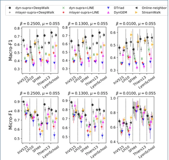
Figure 2 shows the prediction performance of the eight methods considered, for all data sets and SIR parameters considered. The dyn-supra representation com-bined with DeepWalk yields almost always the highest value both for Macro-F1 and Micro-F1, except for the LH10 data set (the smallest data set, see Table 1). We moreover observe that: (i) for a given static embedding method, the dyn-supra supra-adjacency representation gives better results than the baseline (mlayer-supra) one; and (ii) for a given supra-adjacency representation, DeepWalk performs better than LINE. [2]_{https://github.com/tangjianpku/LINE} [3]_{https://github.com/luckiezhou/DynamicTriad} [4]_{http://www-scf.usc.edu/∼nkamra/} [5]_{https://github.com/ferencberes/online-node2vec} [6]_{https://github.com/aditya-grover/node2vec}

0.0

0.2

0.4

0.6

0.8

1.0

0.0

0.2

0.4

0.6

0.8

1.0

dyn-supra+DeepWalk

mlayer-supra+DeepWalk

dyn-supra+LINE

mlayer-supra+LINE

DTriad

DynGEM

Online-neighbor

StreamWalk

InVS15LH10SFHHThiers13

_LyonSchool

0.3

0.4

0.5

0.6

0.7

0.8

Macro-F1

= 0.2500, = 0.055

InVS15LH10SFHHThiers13

_LyonSchool

0.3

0.4

0.5

0.6

0.7

0.8

= 0.1300, = 0.055

InVS15LH10SFHHThiers13

_LyonSchool

0.3

0.4

0.5

0.6

= 0.0100, = 0.055

InVS15LH10SFHHThiers13

_LyonSchool

0.5

0.6

0.7

0.8

0.9

Micro-F1

= 0.2500, = 0.055

InVS15LH10SFHHThiers13

_LyonSchool

0.5

0.6

0.7

0.8

0.9

= 0.1300, = 0.055

InVS15LH10SFHHThiers13

_LyonSchool

0.4

0.6

0.8

1.0

= 0.0100, = 0.055

Figure 2: Prediction performance of each method, for each data set and for various β, at fixed µ = 0.055. The results at fixed β and for various µ are shown as a Supplementary Figure. The top and bottom row give the obtained values of Macro-F1 and Micro-F1, respectively. Error bars give the standard deviation computed over the realizations of the SIR process and the embeddings.

4.3.2 Epidemic impact and epidemic curves

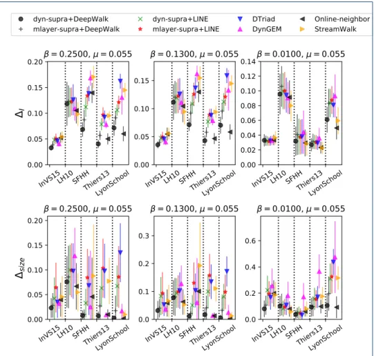
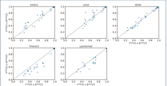
Figure 3 confirms the results of Fig. 2 from the point of view of the discrepancy measures between predicted and real epidemic curves and from the point of view of the error in the predicted final epidemic size: ∆I and ∆size are small for most methods, data sets and parameter values, and in particular the smallest error is most often obtained for the dyn-supra+DeepWalk method. For this method, Figure 4 shows moreover scatterplots of the predicted vs. real final epidemic size, for all data sets: in each plot, epidemic parameters have been varied to yield a large diversity of final epidemic sizes, showing that the predicted and real outcomes are very strongly correlated.

Figures 5 and 6 give a more qualitative illustration of the performance of our method in the reconstruction of the epidemic curves, highlighting as well the ca-pacity of the method to recover the timing of epidemic peaks. This is particularly relevant, as heights and timings of peaks in the number of infectious determine

0.0

0.2

0.4

0.6

0.8

1.0

0.0

0.2

0.4

0.6

0.8

1.0

dyn-supra+DeepWalk

mlayer-supra+DeepWalk

dyn-supra+LINE

mlayer-supra+LINE

DTriad

DynGEM

Online-neighbor

StreamWalk

InVS15LH10SFHHThiers13

_LyonSchool

0.00

0.05

0.10

0.15

0.20

I

= 0.2500, = 0.055

InVS15LH10SFHHThiers13

_LyonSchool

0.00

0.05

0.10

0.15

= 0.1300, = 0.055

InVS15LH10SFHHThiers13

_LyonSchool

0.00

0.02

0.04

0.06

0.08

0.10

0.12

0.14

= 0.0100, = 0.055

InVS15LH10SFHHThiers13

_LyonSchool

0.00

0.05

0.10

0.15

0.20

siz

e

= 0.2500, = 0.055

InVS15LH10SFHHThiers13

_LyonSchool

0.0

0.1

0.2

0.3

= 0.1300, = 0.055

InVS15LH10SFHHThiers13

_LyonSchool

0.0

0.2

0.4

0.6

= 0.0100, = 0.055

Figure 3: Prediction performance of each method in terms of epidemic impact, for each data set and for various β, at fixed µ = 0.055. The results at fixed β and for various µ are shown as a Supplementary Figure. The top and bottom row show respectively the cumulative discrepancy between the real and predicted epidemic curves ∆I and the discrepancy between the final epidemic sizes ∆size. Error bars give the standard deviation computed over the realizations of the SIR process and the embeddings.

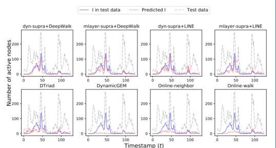
the eventual burden on the healthcare system. Figure 5 first shows that the dyn-supra+DeepWalk method recovers well the periods of large and small number of infectious individuals for all data sets and over a wide range of parameter val-ues. Moreover, Figure 6 shows that the four methods combining a supra-adjacency representation with either DeepWalk or LINE yield good results, while the four other methods strongly underestimate the largest epidemic peak, predicting epi-demic curves that spread out the epiepi-demic impact more evenly over the whole timeline, and thus yielding a less accurate information in terms of size and timing of the largest epidemic burden.

0.0 0.2 0.4 0.6 0.8 1.0 0.0 0.2 0.4 0.6 0.8 1.0 I pr ed(T )+ R pr ed(T ) InVS15 0.0 0.2 0.4 0.6 0.8 1.0 0.0 0.2 0.4 0.6 0.8 1.0 LH10 0.0 0.2 0.4 0.6 0.8 1.0 Ireal_{(T) + R}real_(T) 0.0 0.2 0.4 0.6 0.8 1.0 SFHH 0.0 0.2 0.4 0.6 0.8 1.0 Ireal_{(T) + R}real_(T) 0.0 0.2 0.4 0.6 0.8 1.0 I pr ed(T )+ R pr ed(T ) Thiers13 0.0 0.2 0.4 0.6 0.8 1.0 Ireal_{(T) + R}real_(T) 0.0 0.2 0.4 0.6 0.8 1.0 LyonSchool

Figure 4: Scatterplots of the final predicted epidemic size (number of infectious and recovered nodes at the end of the data set), vs. the real one. Each point corresponds to one simulation, and we vary the epidemic parameters in order to scan a wide range of outcomes. Here we use the dyn-supra+DeepWalk method. The Pearson correlation coefficients for the predicted vs. real sizes are 0.957 for InVS15, 0.88 for LH10, 0.98 for SFHH, 0.96 for Thiers13 and 0.95 for LyonSchool.

0.0

0.2

0.4

0.6

0.8

1.0

Timestamp (t)

0.0

0.2

0.4

0.6

0.8

1.0

Number of active nodes

I in test data

Predicted I

Test data

0

50

100

0

100

200

SFHH

= 0.2500, = 0.055

0

100

200

0

100

200

Thiers13

= 0.2500, = 0.055

0

50

100

0

50

100

150

200

LyonSchool

= 0.2500, = 0.055

0

50

100

0

100

200

= 0.1300, = 0.100

0

100

200

0

100

200

= 0.1300, = 0.100

0

50

100

0

50

100

150

200

= 0.1300, = 0.100

0

50

100

0

100

200

= 0.1300, = 0.055

0

100

200

0

100

200

= 0.1300, = 0.055

0

50

100

0

50

100

150

200

= 0.1300, = 0.055

0

50

100

0

100

200

= 0.1300, = 0.010

0

100

200

0

100

200

= 0.1300, = 0.010

0

50

100

0

50

100

150

200

= 0.1300, = 0.010

Figure 5: Example of predicted timelines of the number of active nodes in the infectious state, for several data sets and (β, µ) parameter values, for the dyn-supra+DeepWalk method. The blue, red and gray lines are respectively the num-ber of actual active nodes in state I in the test data, the numnum-ber of predicted active nodes in state I and the number of active nodes in the test data at time t. Note that the number of active nodes in the test data is almost the same as the total number of active nodes, as the training data is of small size (ρ = 1, i.e., |D| = |V |).

0.0 0.2 0.4 0.6 0.8 1.0

Timestamp (t)

Number of active nodes

I in test data Predicted I Test data

0 50 100 0 100 200 dyn-supra+DeepWalk 0 50 100 0 100 200 mlayer-supra+DeepWalk 0 50 100 0 100 200 dyn-supra+LINE 0 50 100 0 100 200 mlayer-supra+LINE 0 50 100 0 100 200 DTriad 0 50 100 0 100 200 DynamicGEM 0 50 100 0 100 200 Online-neighbor 0 50 100 0 100 200 Online-walk

Figure 6: Example of predicted timelines of the number of active nodes in the infectious state, for the SFHH (conference) data set for the various methods. Here (β, µ) = (0.13, 0.055) and ρ = 1. Line colors have the same meaning as in Fig. 5.

0.0

0.2

0.4

0.6

0.8

1.0

0.0

0.2

0.4

0.6

0.8

1.0

dyn-supra+DeepWalk

mlayer-supra+DeepWalk

dyn-supra+LINE

mlayer-supra+LINE

5

10 15

0.4

0.5

0.6

Macro-F1

50

100

d

0.3

0.4

0.5

0.6

5

10 15

0.4

0.5

0.6

0.7

0.0

0.2

0.4

0.6

0.8

1.0

0.0

0.2

0.4

0.6

0.8

1.0

5

10 15

0.03

0.04

0.05

0.06

I

50

100

d

0.03

0.04

0.05

0.06

5

10 15

0.03

0.04

0.05

0.06

Figure 7: Results of the hyper-parameter sensitivity on the Macro-F1 and ∆I performance measures for the InVS15 data set. Bars indicate the standard devi-ation. Here (β, µ) = (0.13, 0.055).

4.3.3 Sensitivity analysis

We now investigate the effect of the hyper-parameters of the supra-adjacency repre-sentation (the weight ω of self-coupling edges) and of the embedding (the embedding dimension d). We show in Fig. 7 the results obtained for two performance measures, for the InVS15 data set and (β, µ) = (0.13, 0.055), but we have confirmed the same tendency for the other data sets, parameter values and for the Micro-F1 and ∆size measures. The results show that the performance of dyn-supra+DeepWalk is very stable with respect to changes in ω. The performance is also stable on a wide range of embedding dimensions, and decreases when it becomes smaller than ≈ 50. Over-all, dyn-supra+DeepWalk remains very effective without the need for fine-tuning ω or d.

Figure 7 also shows the effect of increasing the parameter ρ, i.e., of being able to observe a larger fraction of active nodes. The performance slightly increases with ρ and in particular dyn-supra+DeepWalk consistently yields the best result at all values of ρ.

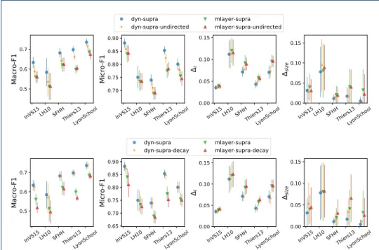
As mentioned above, we finally consider two variations if the dyn-supra repre-sentation: (i) we regard edges as directed towards increasing timestamps (dyn-supra-directed ); (ii) we let the weight of an edge decay with increasing temporal lag between the active nodes it links, e.g., we modulate the edge weight according

0.0 0.2 0.4 0.6 0.8 1.0 0.0 0.2 0.4 0.6 0.8 1.0 dyn-supra

dyn-supra-undirected mlayer-supramlayer-supra-undirected

InVS15 LH10 SFHHThiers13_LyonSchool

0.5 0.6 0.7

Macro-F1

InVS15 LH10 SFHHThiers13_LyonSchool

0.70 0.75 0.80 0.85 0.90 Micro-F1

InVS15 LH10 SFHHThiers13_LyonSchool

0.00 0.05 0.10 0.15

I

InVS15 LH10 SFHHThiers13_LyonSchool

0.00 0.05 0.10 0.15 siz e 0.0 0.2 0.4 0.6 0.8 1.0 0.0 0.2 0.4 0.6 0.8 1.0 dyn-supra

dyn-supra-decay mlayer-supramlayer-supra-decay

InVS15 LH10 SFHHThiers13_LyonSchool

0.5 0.6 0.7

Macro-F1

InVS15 LH10 SFHHThiers13_LyonSchool

0.65 0.70 0.75 0.80 0.85 0.90 Micro-F1

InVS15 LH10 SFHHThiers13_LyonSchool

0.00 0.05 0.10 0.15

I

InVS15 LH10 SFHHThiers13_LyonSchool

0.00 0.05 0.10 0.15 siz e

Figure 8: Effect of the variations in the supra-adjacency representation, for the DeepWalk embedding. Here (β, µ) = (0.13, 0.055). Top: effect of using undirected edges. Bottom: effect of introducing weights depending on time difference. Bars indicate the standard deviation.

to the reciprocal of the lag (dyn-supra-decay). We also consider these variations for mlayer-supra representation, yielding directed and mlayer-supra-decay, respectively. Notice that, in the mlayer-supra method, the supra-adjacency edges representing temporal edges are actually not affected by these variations. We report in Fig. 8 the results for (β, µ) = (0.13, 0.055) and for the DeepWalk embed-ding, as DeepWalk overall yielded the best results. We checked that the results of Fig. 8 hold similarly for the LINE embeddings.

Figure 8 indicates that using undirected edges slightly worsens the performance of both dyn-supra and mlayer-supra methods. Introducing weights that depend on the time difference between active edges also worsens the performance for mlayer-supra, with little effect on dyn-supra. Overall, the original dyn-supra method with directed edges and using only the weights of the original temporal edges yields the highest prediction performance.

5 Conclusion

We have introduced a new method to recover the dynamical evolution of a single instance of a process that has taken place on a known temporal network, from partial observations and without information on the nature of the process itself except from the set of possible states of the nodes. Our strategy is based on leveraging the field of node embedding techniques and on the introduction of a new method for embedding nodes of temporal networks aimed at providing low-dimensional feature vectors that are informative of dynamical processes occurring over temporal networks.

Our method first maps the temporal network to a modified supra-adjacency rep-resentation, which, despite being a static network, contains all the temporal infor-mation of the temporal network, and in particular preserves the paths on which the process unfolds. As this representation yields a static graph among the active nodes, which are pairs of the form (node of the temporal network, time of inter-action), it enables the use of embedding techniques for static networks. We choose to use DeepWalk, as it is a simple and paradigmatic algorithm based on random walks and thus particularly suited to explore the neighborhood of the nodes of the supra-adjacency representation in a way relevant to the dynamical process on the network. We finally frame the inference of the dynamical state of all active nodes from a set of observations as a supervised classification task.

We have shown the performance of our method on the case of an epidemic-like model on empirical temporal networks and compared it with other state of the art methods. Our method consistently yields very good classification performance in a robust way across data sets and process parameters, without fine-tuning hyper-parameters.

Our results show that it is possible, without any knowledge of the precise nature of the process nor of its parameters, to recover crucial information on its outcome, even with a very limited number of observations (for most of our results, each node is observed on average once). Note in particular that our method assumes no knowledge of which transitions between states actually occur in the real dynamics: this means that the predicted sequence of states of each individual node might yield ”forbidden” transitions (e.g., in the SIR example, transitions from I to S or from R to I). Nevertheless, we have shown that the outcome of the classification task gives a good estimation of the actual dynamics, as quantified both by usual measures of prediction task performance and measures focusing more on the epidemic burden, such as the cumulative discrepancy between predicted and real epidemic curves and the difference between predicted and real final epidemic sizes. We have also shown that the height and timing of the epidemic curve, which in fine determines the period of worst expected burden on the healthcare system during an epidemic, are also well reproduced in our framework, while the other embedding methods for temporal networks predict a more spread out epidemic over the whole temporal window, with an underestimation of the epidemic peak height.

Our method has the clear limitation that we assume the whole temporal network to be known. Although a full observation of the contact patterns of individuals could be envisioned in some specific controlled settings such as hospitals, this is not generally the case. Further work will address this limitation by considering the effect of noise and errors in the temporal network data, and by considering the case in which only a (more or less detailed) set of statistics of the temporal network is known. Moreover, a related limitation of our investigations concerns our prepro-cessing of the original temporal network: indeed, we have chosen to aggregate the network data on consecutive 600 seconds time intervals, in order to smoothen out short term noisy dynamics. As far as SIR processes are concerned, this aggregation can arguably have an effect on the epidemic dynamics and on prediction perfor-mance, as the aggregated data has less noise than the raw data, and loses some information on which paths are time-respecting. It would thus be interesting for in-stance to systematically monitor the performance of the procedure as a function of

the temporal aggregation window length. Noise could also impact the quality of the sampling (e.g., observational errors), and we will check its impact on our method’s performance. Further work will also address different sampling strategies such as a sampling concentrated at early times, or focused on few specific “sentinel” nodes followed at all times, or of a whole snapshot of the system but only at a specific time. This could yield interesting insights on how to optimize surveillance strategies in more realistic settings. Another interesting direction for further work would be to consider a dynamical process unfolding over a streamed temporal network, where information on both the temporal edges and on the partially observed nodes’ states are available in a streaming fashion. This would yield more complex prediction tasks based on past information, only.

Finally, since our method is largely agnostic with respect to the specific dynamical process, we will consider other processes such as other models of disease propagation, complex contagion phenomena or opinion formation.

Declarations

Availability of data

We have used publicly available data sets.

Competing interests

The authors declare that they have no competing interests.

Author’s contributions

A.B., C.C., M.O. designed the study. K.S. implemented the embedding methods, the numerical simulations and analyzed the results. All authors wrote and approved the final version of the manuscript.

Funding

This study was partially supported by the Lagrange Project of the ISI Foundation funded by CRT Foundation to CC. It was partially supported by the ANR project DATAREDUX (ANR-19-CE46-0008-01) to AB.

Author details

1_{University of Tsukuba, Tsukuba, Japan.} 2_{Aix Marseille Univ, Universit´e de Toulon, CNRS, CPT, Turing Center for} Living Systems, Marseille, France. 3_{Tokyo Institute of Technology, Tokyo, Japan.} 4_{University of Turin, Turin, Italy.} 5_{ISI Foundation, Turin, Italy.}

References

1. Albert, R., Barab´asi, A.-L.: Statistical mechanics of complex networks. Rev. Mod. Phys. 74(1), 47 (2002) 2. Newman, M.E.: The structure and function of complex networks. SIAM Rev. 45(2), 167–256 (2003) 3. Barrat, A., Barth´elemy, M., Vespignani, A.: Dynamical Processes on Complex Networks. Cambridge University

Press, Cambridge (2008)

4. Pastor-Satorras, R., Castellano, C., Van Mieghem, P., Vespignani, A.: Epidemic processes in complex networks. Rev. Mod. Phys. 87(3), 925 (2015)

5. Holme, P., Saram¨aki, J.: Temporal networks. Physics Reports 519, 97–125 (2012)

6. Holme, P.: Modern temporal network theory: a colloquium. Eur. Phys. J. B 88(9), 234 (2015)

7. Sundareisan, S., Vreeken, J., Prakash, B.A.: Hidden hazards: Finding missing nodes in large graph epidemics. In: SDM, pp. 415–423 (2015)

8. Xiao, H., Aslay, C., Gionis, A.: Robust cascade reconstruction by steiner tree sampling. In: ICDM, pp. 637–646 (2018). doi:10.1109/ICDM.2018.00079

9. Sefer, E., Kingsford, C.: Diffusion archeology for diffusion progression history reconstruction. KAIS 49(2), 403–427 (2016)

10. Feizi, S., Medard, M., Quon, G., Kellis, M., Duffy, K.: Network infusion to infer information sources in networks. IEEE TNSE 6(3), 402–417 (2018)

11. Chen, Z., Tong, H., Ying, L.: Inferring full diffusion history from partial timestamps. IEEE TKDE, 1–1 (2019) 12. Altarelli, F., Braunstein, A., Dall’Asta, F., Ingrosso, A., Zecchina, R.: The patient-zero problem with noisy

observations. JSTAT 2014(10), 10016 (2014)

13. Rozenshtein, P., Gionis, A., Prakash, B.A., Vreeken, J.: Reconstructing an epidemic over time. In: KDD, pp. 1835–1844 (2016)

14. Xiao, H., Rozenshtein, P., Tatti, N., Gionis, A.: Reconstructing a cascade from temporal observations. In: SDM, pp. 666–674 (2018)

15. Cai, H., Zheng, V.W., Chang, K.C.: A comprehensive survey of graph embedding: Problems, techniques, and applications. IEEE TKDE 30(9), 1616–1637 (2018)

16. Goyal, P., Ferrara, E.: Graph embedding techniques, applications, and performance: A survey. Knowledge-Based Systems 151, 78–94 (2018)

17. Goyal, P., Chhetri, S.R., Canedo, A.: dyngraph2vec: Capturing network dynamics using dynamic graph representation learning. Knowledge-Based Systems (2019). doi:10.1016/j.knosys.2019.06.024 18. Krings, G., Karsai, M., Bernhardsson, S., Blondel, V.D., Saram¨aki, J.: Effects of time window size and

placement on the structure of an aggregated communication network. EPJ Data Science 1(1), 4 (2012) 19. Holme, P.: Epidemiologically optimal static networks from temporal network data. PLOS Computational

Biology 9(7), 1–10 (2013). doi:10.1371/journal.pcbi.1003142

20. Pfitzner, R., Scholtes, I., Garas, A., Tessone, C.J., Schweitzer, F.: Betweenness preference: Quantifying correlations in the topological dynamics of temporal networks. Phys. Rev. Lett. 110, 198701 (2013). doi:10.1103/PhysRevLett.110.198701

21. Scholtes, I., Wider, N., Garas, A.: Higher-order aggregate networks in the analysis of temporal networks: path structures and centralities. The European Physical Journal B 89(3), 61 (2016)

22. Lambiotte, R., Rosvall, M., Scholtes, I.: From networks to optimal higher-order models of complex systems. Nature Physics 15(4), 313–320 (2019). doi:10.1038/s41567-019-0459-y

23. Valdano, E., Ferreri, L., Poletto, C., Colizza, V.: Analytical computation of the epidemic threshold on temporal networks. Phys. Rev. X 5, 021005 (2015). doi:10.1103/PhysRevX.5.021005

24. Kivel¨a, M., Cambe, J., Saram¨aki, J., Karsai, M.: Mapping temporal-network percolation to weighted, static event graphs. Scientific Reports 8(1), 12357 (2018)

25. Badie-Modiri, A., Karsai, M., Kivel¨a, M.: Efficient limited-time reachability estimation in temporal networks. Phys. Rev. E 101, 052303 (2020). doi:10.1103/PhysRevE.101.052303

26. Perozzi, B., Al-Rfou, R., Skiena, S.: Deepwalk: Online learning of social representations. In: KDD, pp. 701–710 (2014)

27. Grover, A., Leskovec, J.: Node2vec: Scalable feature learning for networks. In: KDD, pp. 855–864 (2016) 28. Castellano, C., Fortunato, S., Loreto, V.: Statistical physics of social dynamics. review of Modern Physics 81,

591–646 (2009)

29. Pastor-Satorras, R., Castellano, C., Mieghem, P.V., Vespignani, A.: Epidemic processes in complex networks. Rev. Mod. Phys. 87(3), 925 (2015)

30. Keeling, M.J., Rohani, P.: Modeling Infectious Diseases in Humans and Animals. Princeton University Press, Princeton (2008)

31. G´omez, S., D´ıaz-Guilera, A., G´omez-Garde˜nes, J., P´erez-Vicente, C.J., Moreno, Y., Arenas, A.: Diffusion dynamics on multiplex networks. Phys. Rev. Lett. 110, 028701 (2013). doi:10.1103/PhysRevLett.110.028701 32. Kivel¨a, M., Arenas, A., Barthelemy, M., Gleeson, J.P., Moreno, Y., Porter, M.A.: Multilayer networks. Journal

of Complex Networks 2(3), 203–271 (2014)

33. Tang, J., Qu, M., Wang, M., Zhang, M., Yan, J., Mei, Q.: Line: Large-scale information network embedding. In: WWW, pp. 1067–1077 (2015)

34. Zhou, L., Yang, Y., Ren, X., Wu, F., Zhuang, Y.: Dynamic network embedding by modeling triadic closure process. In: AAAI (2018)

35. Goyal, P., Kamra, N., He, X., Liu, Y.: Dyngem: Deep embedding method for dynamic graphs. arXiv preprint arXiv:1805.11273 (2018)

36. B´eres, F., Kelen, D.M., P´alovics, R., Bencz´ur, A.A.: Node embeddings in dynamic graphs. Applied Network Science 4(1), 64 (2019)

37. Cattuto, C., Van den Broeck, W., Barrat, A., Colizza, V., Pinton, J., Vespignani, A.: Dynamics of person-to-person interactions from distributed rfid sensor networks. PLOS ONE 5(7), 11596 (2010)

38. G´enois, M., Barrat, A.: Can co-location be used as a proxy for face-to-face contacts. EPJ Data Science 7(1), 11 (2018)

39. Pedregosa, F., Varoquaux, G., Gramfort, A., Michel, V., Thirion, B., Grisel, O., Blondel, M., Prettenhofer, P., Weiss, R., Dubourg, V., Vanderplas, J., Passos, A., Cournapeau, D., Brucher, M., Perrot, M., Duchesnay, ´E.: Scikit-learn: Machine learning in Python. JMLR 12, 2825–2830 (2011)