HAL Id: hal-02130468
https://hal.archives-ouvertes.fr/hal-02130468
Submitted on 23 May 2020
HAL is a multi-disciplinary open access
archive for the deposit and dissemination of
sci-entific research documents, whether they are
pub-lished or not. The documents may come from
teaching and research institutions in France or
L’archive ouverte pluridisciplinaire HAL, est
destinée au dépôt et à la diffusion de documents
scientifiques de niveau recherche, publiés ou non,
émanant des établissements d’enseignement et de
recherche français ou étrangers, des laboratoires
One-step compact skeletonization
Bastien Durix, Géraldine Morin, Sylvie Chambon, Jean-Luc Mari, Kathryn
Leonard
To cite this version:
Bastien Durix, Géraldine Morin, Sylvie Chambon, Jean-Luc Mari, Kathryn Leonard. One-step
compact skeletonization. 40th Annual Conference of the European Association for Computer Graphics
-Eurographics 2019, May 2019, Genoa, Italy. pp.1-5, �10.2312/egs.20191005�. �hal-02130468�
EUROGRAPHICS 2019/ P. Cignoni and E. Miguel
One-step compact skeletonization
B. Durix1and G. Morin1and S. Chambon1and J.-L. Mari3and K. Leonard2
1IRIT-University of Toulouse, CNRS, France
2Occidental College, Los Angeles, CA, USA
3Aix Marseille Univ, UniversiteÌ ˛A de Toulon, CNRS, LIS, Marseille, France
Abstract
Computing a skeleton for a discretized boundary typically produces a noisy output, with a skeletal branch produced for each boundary pixel. A simplification step often follows to reduce these noisy branches. As a result, generating a clean skeleton is usually a 2-step process. In this article, we propose a skeletonization process that produces a clean skeleton in the first step, avoiding the creation of branches due to noise. The resulting skeleton compares favorably with the most common pruning methods on a large database of shapes. Our process also reduces execution time and requires only one parameter, ε, that designates the desired boundary precision in the Hausdorff distance.
1. Introduction
The interior Blum medial axis [Blu67] captures the geometry of the boundary of a two- or three-dimensional shape in a lower-dimensional skeleton together with a radius function defined on the skeleton that encodes the distance to the boundary. The skele-ton is given by the closure of the set of centers of the maxi-mal balls inside the shape, where a maximaxi-mal ball passes through at least two boundary points. The radius function stores the as-sociated radius of each maximal ball. The medial axis is use-ful in shape recognition and analysis applications, primarily in 2D [Sid99,Sun03,Bai08,Xu,10,Leo16], in part because the skele-tal branches decompose a shape into sub-parts. A major drawback is that skeletonization of discretized boundaries typically creates branches that describe the small fluctuations of the boundary gen-erated by discretization, and as such are uninformative about the shape. Our work introduces a new method that constructs only in-formative branches that capture meaningful geometry of the bound-ary. See Figure1.
(a) Classical Voronoï skeleton (b) Proposed skeletonization
Figure 1: Illustration of the classical problem of skeletons on a rasterized shape: the presence of uninformative branches.
Many skeletonization methods have been proposed (see [Sah15] for a survey), some of which compute a clean skeleton directly. For example, [LMT15] combines the ridges of the distance map and the centers of the maximal balls to compute the skeleton on the grid of pixels. As happens with thinning methods, the skele-ton is a subset of the pixel grid and therefore has width of one pixel. Another approach that produces point skeletons modifies the boundary itself, as in the circular boundary representation [Aic09] proposed by Aichholzer et al.. The resulting skeleton avoids many uninformative branches, but the construction is complicated: con-verting the boundary into arcs requires that the boundary is repre-sented by polynomial splines, which are then converted into circu-lar arcs based on a chosen parameter. In contrast, our method uses the information of the discrete boundary directly without any pre-processing.
In this article, we build on one of the most common methods, the Voronoï skeletonization [Ogn92], that estimates a Voronoï diagram from a sampling of the boundary and approximates the medial axis using the diagram’s interior vertices and edges. A medial point is then a Voronoï vertex, with radius equal to the distance from the Voronoï vertex to the associated boundary points. This method is very precise if the sampling of the boundary is finer than the local feature size [Att97]. It is also fast due to the optimization of the Voronoï diagram algorithm.
Unfortunately, the Voronoï approach often produces a skeleton with many uninformative branches. The usual approach to this problem is to prune the less important parts of the skeleton. The pruning criteria typically rely on evaluating properties of the medial circle centered at the Voronoï point. We present the three most com-mon pruning criteria. The λ-medial axis [Cha05] removes a circle if its associated boundary points are contained in a circle of radius
B. Durix, G. Morin, S. Chambon, J.-L. Mari, K. Leonard / One-step compact skeletonization
λ (later extended to a new definition of the medial axis [Cha09]). The θ-homotopy medial axis [Sud05], evaluates the angle between the medial point and its associated boundary points. If the angle is less than θ, the circle is removed. Finally, the scale-axis-transform [Gie09] expands each circle by a multiplicative factor s and then removes any circle contained inside another one.
These three methods have the same disadvantages. First, the topology of the resulting skeleton can be modified by the prun-ing algorithm: for example holes can be closed with the scale-axis-transform. Second, the choice of the parameter used for the prun-ing is difficult, because it does not have an intuitive interpretation (cf. Figure2). Third, these pruning methods do not distinguish reli-ably between noise and small geometric details (cf. Figure3) which means that important details can be lost in pruning. Finally, these methods are applied after the computation of the skeleton, so addi-tional computation time is necessary.
(a) θ-homotopy medial axis,
θ =6π
18, 47 branches
(b) θ-homotopy medial axis,
θ =7π 18, 17 branches (c) Proposed Propagation, ε = 1px, 23 branches (d) Proposed Propagation, ε = 1.5px, 13 branches
Figure 2: (Top) Difficulty of selecting the θ parameter: here, it is hard to predict that increasing θ will erase the branches represent-ing the top of the head. (Bottom) In the proposed skeletonization, the parameter ε is the Hausdorff distance (HD) between the origi-nal shape and the approximated shape represented by the skeleton. It therefore describes the desired precision of the approximation.
In this article, we propose a novel 2D skeletonization method, an improved version of a propagation algorithm introduced in [Dur19]. This algorithm avoids generating uninformative branches and therefore requires no pruning. The approach propa-gates a Voronoï-generated medial circle inside the shape, insuring continuous contact with the boundary. Furthermore, the circle is propagated only in so-called informative directions as determined by the desired precision ε. This threshold, ε, is the only param-eter of our algorithm. We guarantee that the resulting skeleton-generated shape represents an ε-approximation of the original shape, in terms of the Hausdorff distance, as in [ZSC∗14], but with-out pruning. For pixelated shapes, such as those extracted from im-ages, we will have an ε-px approximation of the shape. We intro-duce the proposed algorithm in Section2and then compare our results with pruning methods in Section3.
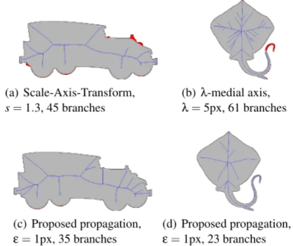
(a) Scale-Axis-Transform, s= 1.3, 45 branches (b) λ-medial axis, λ = 5px, 61 branches (c) Proposed propagation, ε = 1px, 35 branches (d) Proposed propagation, ε = 1px, 23 branches
Figure 3: Some pruning methods (here scale-axis-transform and λ-medial axis) delete shape details while keeping noise on the skele-ton. The proposed method preserves all details of the shape while removing the noise.
2. Voronoï skeletonization by propagation
We construct the skeletonization by propagating the skeleton from an initial circle. Every skeletal circle passes through three or more boundary points. For each pair of these points, a potential neighbor circle can be computed that passes through both points (e.g., be-tween B1and B2in Figure4). We avoid propagating in directions
due to noise by ensuring that the boundary points between the two points are not too close to the original circle (for example between B0and B1on Figure4). Algorithm1elaborates on this reasoning.
We first describe the goal of each algorithmic function, then present the properties of the algorithm.
P B0
B1
B2
2ε
Figure 4: Desirable (open) directions on the circle. The red dashed circle has radius2ε larger than the black circle. The sequence of points between B0, B1 is inside the red dashed circle, thus these
points are ε-points, and the direction between B0 and B1 is not
open. Here, two open directions remain (between B1and B2, and,
B2and B0).
2.1. Functions
Algorithm1is based on the following functions:
f irst_center:provides a first circle center in the shape that passes through three boundary points. Starting with any point in the shape interior and its inscribed circle, we can perturb the point until the inscribed circle passes through three points of the boundary and is
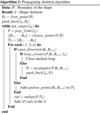
Algorithm 1: Propagating skeleton algorithm Data: B : Boundary of the shape
Result: S : Shape skeleton 1 P0= f irst_point(B) 2 push_back(lp, P0) 3 while not_empty(lp) do 4 P= pop_ f ront(lp) 5 {B1, · · · , Bn} = closest_points(P, B) 6 Pε= {B1, · · · , Bn} 7 For each i ∈ [1; n] do 8 If open_direction(Bi, Bi+1) 9 If loop_closure(P, Bi, Bi+1, lp)
10 Close skeletal loop 11 Else
12 Pi= propagate(P, Bi, Bi+1)
13 push_back(lp, Pi)
14 End
15 Else
16 Add epsilon_points(Bi, Bi+1) to Pε
17 End
18 rad= radius(P, Pε)
19 Add (P, rad) to the S 20 End
21 end
therefore maximal. See Figure5. This step returns the circle center, which initializes the algorithm. Note that the resulting skeleton is independent of the starting point.
closest_points:returns the points of the boundary that lie on the circle. As the distances on a computer cannot be exact, we use the machine precision as a threshold on the distance to the circle to de-termine which points are on the circle.
epsilon_points: Between two boundary points Bk and Bk+1
be-longing to a circle, if all intermediate boundary points between Bk
and Bk+1are at most at distance 2ε to the circle, we call them ε-points associated to that circle (cf. Figure4) and they are considered covered (these boundary points will be at most at distance 2ε of the circle). If there exists at least one point that is beyond 2ε, then no ε-point exists between the two closest points.
radius:estimates the radius associated with a circle. We take the average between the circle radius and the distance to the farthest ε-point, in order to minimize the Hausdorff distance between the shape modeled by the skeleton and the initial shape.
loop_closure:handles the loops in the skeleton. For each circle center, we check if there exists a neighbor circle center in the list of centers lp. By definition, neighboring centers share a pair of closest
points.
open_direction: determines directions for possible propagation. We use ε-points is to check whether or not a direction is open, as explained in Figure4.
propagate: finds the next circle. Given an open direction Bk,
Bk+1, we seek the next circle center on the bisector of [BkBk+1]
(cf. Fig. 5(c)). The next circle passes through Bk, Bk+1, and a
new point of the boundary, and does not strictly contain any other boundary point. A B C D Pa (a) A B C Pa Pb (b) A B C Pb Pc (c)
Figure 5: First circle center estimation. (a) Identifying the shape interior using a corner D of the bounding box and the closest point A on the boundary. The first point will be on the semi-line passing through A with direction ~DA. (b) Identifying a point Pbon the
semi-line[APb), such that the circle centered in Pb with radiuskAPbk,
contains a point C of the boundary and there is no point of the boundary inside the circle. (c) Identifying Pcon the line bisector of
[AC] so that the circle centered in Pcis maximal.
2.2. Properties
The resulting skeleton guarantees the following properties: 1. Each circle found is a circle of the Voronoï diagram: it is a
circle that passes through three or more boundary points and does not contain any other point.
2. Each edge between two circles is a Voronoï edge: since two circles share two boundary points, their Voronoï cells are neigh-bors, thus the edge is joining their centers is a Voronoï edge. 3. The distance from each point of the boundary to a circle is
at most ε: each ε-point is at most at distance ε to the associated circle, according to the radius computation.
4. Choosing ε = 0 returns the full Voronoï diagram: a circle cannot have any ε-point, thus all circles have only closest points. Thus, every point of the boundary is on a Voronoï circle, which means that we have the full internal Voronoï diagram.
5. The connectivity of the skeleton is the same as the full in-ternal Voronoï diagram: Our method consists in computing only a partial Voronoï diagram, closing some propagation di-rections. Closing a direction, made of consecutive ε-points, is topologically equivalent to replacing the consecutive ε-points by the closest points they link. Thus, our skeletonization method returns a skeleton that is the Voronoï skeleton on a simplified boundary that is homotopy equivalent to the original boundary. 6. The complexity is proportional to N2, where N is the number of boundary points: The propagation explores at most all the points of the boundary for each skeletal point, and the number of skeletal points is of the same order as the number of boundary points.
3. Results and comparison
In this section, we compare the skeletonization by propagation with the Voronoï skeletonization pruned by scale-axis transform, λ-medial axis, and θ medial axis. As stated previously, the Voronoï skeletonization is one of the most commonly used methods to con-struct the skeleton of a discretized shape that produces a graph, like our skeleton.
Figure6presents a comparison between the proposed method and the Voronoï skeleton pruned by different methods. Each
B. Durix, G. Morin, S. Chambon, J.-L. Mari, K. Leonard / One-step compact skeletonization
method has one parameter: s for scale-axis-transform, λ for λ-medial axis, θ for θ-λ-medial axis, and ε for our skeletonization. Dif-ferent choices for parameter values will produce a difDif-ferent number of branches. We compare results on 1282 images from the MPEG-7 database [Lat00]. By quantifying the loss of information as a function of the number of branches in the skeleton produced, we evaluate the relevance of the discarded branches to the shape: if a method removes fewer informative branches, the loss of infor-mation should be stable as the number of branches decreases. We observe that only our method respects this criterion, while the prun-ing methods lose more information. Figure7shows some examples using our method. We can see that there are few branches for each skeleton and that the shape is approximated well. The mean com-putation time for each image is 13ms. By comparison, the mean computation for the full Voronoï is 60ms (i.e. with ε = 0), filtering with scale-axis-transform takes between 365ms and 1670ms, with λ-medial axis takes between 103ms and 111ms and with θ-medial axis takes between 207ms and 1450ms to compute, depending on the choice of their respective parameters.
0 200 400 600 800 Number of branches 0 5 10 15 20 25 30 35 Hausdorff distance scale-axis-tranform -medial axis -medial axis skeletonization by propagation 0 200 400 600 800 Number of branches 0 2 4 6 8 10
Percentage of area difference
scale-axis-tranform -medial axis -medial axis skeletonization by propagation
Figure 6: Distance between the original shape and the shape gen-erated by a simplified skeleton with respect to the number of ton branches, for three pruning methods, and our proposed skele-tonization. We consider two criteria: the Hausdorff distance (left) and the relative area of the symmetric difference (right).
Figure 7: Skeletons of some shapes of the MPEG-7 database, com-puted with skeletonization by propagation. We use ε = 1 for each shape. The area modeled by the skeleton is grey, the lost regions are in red, and the boundary in black.
4. Conclusion
In this article, we have presented a new skeletonization method that directly computes a simple skeleton with a low number of branches. We propagate selected Voronoï circles within the shape and discard directions of propagation that represent negligible information, be-low a chosen threshold. Our method is simple to tune, as the only parameter is twice the upper bound of the desired Hausdorff dis-tance between the output shape and the original shape. We have also shown that increasing the value of our parameter decreases the number of branches while limiting loss of shape information as compared to classical pruning methods. In other words, the pre-served skeleton branches retained by our method are highly infor-mative branches.
One direction for future work is the automatic estimation of boundary noise by determining the ε parameter that maximizes the ratio between the number of branches and the information loss. We can see on Figure6that there is an elbow in the black curve (a point with a large change in derivative for each of the graphs). This elbow point should be close to the optimal ε parameter. A second direction is to adapt this algorithm for 3D skeletonization. 3D skeletonization from surface data is even more affected by noise, leading to very complex structures.
References
[Aic09] AICHHOLZER, O.ANDAIGNER, W.ANDAURENHAMMER, F.
ANDHACKL, T.ANDJÜTTLER, B.ANDRABL, M.: Medial axis
com-putation for planar free-form shapes. Comp. Aid. Des. 41, 5 (2009),
339–349.1
[Att97] ATTALI, D.ANDMONTANVERT, A.: Computing and
Simplify-ing 2D and 3D Continuous Skeletons. CVIU 67, 3 (1997).1
[Bai08] BAI, X.ANDLATECKI, L. J.: Path Similarity Skeleton Graph
Matching. PAMI 30, 7 (2008).1
[Blu67] BLUM, H.: A Transformation for Extracting New Descriptors of
Shape. In Symp. on Mod. for the Perc. of Speech and Vis.Form (1967).1
[Cha05] CHAZAL, F.ANDLIEUTIER, A.: The λ-medial Axis. Graphical
Models 67, 4 (2005).1
[Cha09] CHAUSSARD, J.ANDCOUPRIE, M.ANDTALBOT, H.: A
dis-crete λ-medial axis. In Disc. Geometry for Comp. Imagery (2009).2
[Dur19] DURIX, B. AND CHAMBON, S. AND LEONARD, K. AND
MARI, J.-L.ANDMORIN, G.: The propagated skeleton: a robust
detail-preserving approach. In DGCI (2019).2
[Gie09] GIESEN, J.ANDMIKLOS, B.ANDPAULY, M.ANDWORMSER,
C.: The Scale Axis Transform. In Symp. on Comp. Geometry (2009).2
[Lat00] LATECKI, L. J. AND LAKAMPER, R. AND ECKHARDT, T.:
Shape descriptors for non-rigid shapes with a single closed contour. In
CVPR(2000).4
[Leo16] LEONARD, K.ANDMORIN, G.ANDHAHMANN, S.ANDCAR
-LIER, A.: A 2D shape structure for decomposition and part similarity.
In ICPR (2016).1
[LMT15] LEBORGNEA., MILLEJ., TOUGNEL.: Noise-resistant digital
euclidean connected skeleton for graph-based shape matching. Jour. of
Visual Communication and Image Representation 31(2015), 165–176.1
[Ogn92] OGNIEWICZ, R.ANDILG, M.: Voronoi skeletons: Theory and
applications. In CVPR (1992).1
[Sah15] SAHA, P. K.ANDBORGEFORS, G.ANDSANNITI DIBAJA, G.:
A survey on skeletonization algorithms and their applications. PR letters
76, Supplement C (2015).1
[Sid99] SIDDIQI, K.ANDSHOKOUFANDEH, A.ANDDICKINSON, S. J.
ANDZUCKER, S. W.: Shock Graphs and Shape Matching. IJCV 35, 1
(1999).1
[Sud05] SUD, A.ANDFOSKEY, M.ANDMANOCHA, D.:
Homotopy-preserving Medial Axis Simplification. In ACM Symp. on Solid and
Physical Modeling(2005).2
[Sun03] SUNDAR, H.ANDSILVER, D.ANDGAGVANI, N.ANDDICK
-INSON,S.:Skeleton based shape matching and retrieval. In SMI (2003).1
[Xu,10] XU, Y.ANDWANG, B.ANDLIU, W.ANDBAI, X.:
Skele-ton Graph Matching Based on Critical Points Using Path Similarity. In
ACCV(2010).1
[ZSC∗14] ZHUY., SUNF., CHOIY.-K., JÜTTLERB., WANGW.:
Com-puting a compact spline representation of the medial axis transform of a