HAL Id: hal-02435803
https://hal.archives-ouvertes.fr/hal-02435803
Submitted on 11 Jan 2020HAL is a multi-disciplinary open access
archive for the deposit and dissemination of sci-entific research documents, whether they are pub-lished or not. The documents may come from teaching and research institutions in France or abroad, or from public or private research centers.
L’archive ouverte pluridisciplinaire HAL, est destinée au dépôt et à la diffusion de documents scientifiques de niveau recherche, publiés ou non, émanant des établissements d’enseignement et de recherche français ou étrangers, des laboratoires publics ou privés.
Fractal Self-Avoiding Walks
Pascal Préa
To cite this version:
Fractal Self-Avoiding Walks
Pascal Pr´eaLaboratoire d’Informatique Fondamentale de Marseille, LIF, CNRS UMR 7279,
´Ecole Centrale Marseille, Marseille, France
Abstract
For any odd integer K > 1, we define FK, a new family of self-avoiding walks (SAW) on the square
lattice Z ⇥Z, called K-fractal walks. These families have a simple and natural characterization and they seem to all have a critical exponent ⌫ for mean-square displacement in ]0.5, 1[. For small values of K at least , these families are easy to count and it is also very easy to randomly generate a K-fractal walk. In addition, limK!1FKis the set of all SAWs on Z ⇥ Z. We present also some variants of fractal SAWs,
e.g. fractal SAWs on the d-dimensional grid Zd.
Key Words: Self Avoiding Walks, Fractal Structures, Enumeration, Random Generation.
1 Introduction
A walk on a lattice is self-avoiding if it never passes twice through the same vertex. Self-avoiding walks (SAWs) appeared as a model for polymers [10]. They also have applications in statistical physics [11] and in probability theory [13]. Given a lattice (for instance, the hexagonal lattice on plane or the cubic one Z ⇥ Z ⇥ Z in space), the two main questions concerning SAWs on that lattice are:
• What is the number cnof SAWs of length n?
• Given a distribution on the SAWs (for instance the uniform distribution on the SAWs of length n), what is the average distance dnbetween the two extremities of a SAW of length n?
It is conjectured [13] that: • cn⇠ µnn 1
• dn⇠ n⌫
It is strongly believed that the critical exponents and ⌫ depend only on the dimension (and not on the lattice) while the connective constant µ also depends on the lattice.
Despite decades of efforts, these questions remain unsolved, especially in low dimensions. It has re-cently been shown [8] that the connective constant for the hexagonal lattice on plane isp2 +p2. Con-versely, for the square lattice on plane, it is conjectured [12] that the connective constant is the unique positive root of 13x4 7x2 581 = 0 (i.e. q7+p30261
26 ⇡ 2.64). For two-dimensional lattices, it is
conjectured that = 43/32 and that ⌫ = 3/4.
Until now, these conjectures have not been rigorously proved. It is thus natural [1] [2] [6] [7] to define and/or study classes of SAWs which:
• have a natural definition.
• can be easily counted or studied.
In this paper, we introduce new classes of SAWs which satisfy these goals. In Section 2, we give the definition of this new class, then we show how to count these SAWs. In Section 4, we show how to generate random such SAWs and we see that, for these SAWs, the critical exponent ⌫ seems to be < 1. We end by presenting some variants of these SAWs.
2 Definitions
We consider the square grid Z ⇥ Z on plane. A walk is a sequence A = (a0 = (0, 0), a1, . . . an)of vertices
such that, for all i < n, ai and ai+1 are neighbours (i.e. if ai = (xi, yi)and ai+1 = (xi+1, yi+1), then
(xi+1 = xi and yi+1 = yi ± 1) or (yi+1 = yi and xi+1 = xi ± 1)). The walk A is self-avoiding if
i6= j =) ai 6= aj.
Let K be an odd integer > 1. For every positive integer p, we simultaneously partition Z ⇥ Z into squares of side Kp such that for every p > 0, every square of size Kp+1contains K2 squares of size Kp
(see figure 1). Throughout this paper, we will always consider such multi-partitions, and we we call square a part of one of the partitions (a square is of size Kp⇥ Kp).
Figure 1: Partition of Z ⇥ Z for K = 3 Let A be a SAW on Z ⇥ Z, A is K-Fractal (we say it is an FKSAW) if:
1. It does not pass twice through the same square (i.e., once it has left a square, it never comes back in it — Before leaving a square, the walk can, of course, pass through many vertices of this square) 2. When it leaves a square, it is through the middle of a side.
These two conditions have to be verified for any square, of any size. We denote by FK the set of all these
SAWs. We will suppose in addition that one of the two following properties is verified:
• For every k > 0, point (0, 0) is at the center of a square of size Kk. Equivalently, there exists p > 0 and a square of size Kp such that the walk begins at the center of the square and stays inside this
square. We will call these SAWs centered.
• There exists p > 0 and a square of size Kpsuch that the walk begins at the middle of the West side of
the square and ends at the middle of the East side of it. The walk is entirely contained in this square. We will call these SAWs directed.
These two supplementary conditions do not change the fundamental nature of fractal SAWs. The first one yields nice drawings and the second one requires fewer computations to count the SAWs. Clearly, every SAW of length k is a centered 2k + 1-Fractal SAW. So:
Property 1. limK!1FK is the set of all SAWs.
3 Counting Fractal SAW
We first show that, for every odd integer K, K-Fractal SAWs admit a connective constant µK. Then we will
see that, at least for small values of K, the value of µKcan be determined from an enumeration of SAWs in
a K ⇥ K square.
Property 2. For every odd integer K > 1, K-Fractal SAWs admit a connective constant µK.
Proof. The proof is exactly the same that the one for general SAWs (see [13] p. 9-10); we will only give its sketch. Let cK(n) be the number of K-Fractal SAWs of length n. Every K-Fractal SAW of length
n + m is the concatenation of a K-Fractal SAW of length n and of a K-Fractal SAW of length m. So, cK(n+m) cK(n)⇥cK(m), thus log cK(n+m) log cK(n)+log cK(m)and µK = limn!1(cK(n))1/n
exists.
Actually, a Fractal SAW “considers” each square (of size Kp⇥ Kp) as a vertex (it does not pass through
it twice). So, if we look at a FK SAW in a Kp+1⇥ Kp+1square without detailing how is the walk inside
the Kp⇥ Kp squares, it is like looking at a SAW inside a K ⇥ K square. If we look at directed SAW, we
only have to consider two types of SAWs in a K ⇥ K square (see Figure 2): Walks which cross the square from one side to the opposite side.
Walks which turn inside the square.
If we look at centered SAWs, we have to consider in addition the three following types (see Figure 2): Walks which begin at the center of the square and leave it.
Walks which enter the square and do not leave it.
Walks which begin at the center of the square and stay inside it.
- - - 6 r
-b r
b
Figure 2: The five types of SAWs on a 3 ⇥ 3 square
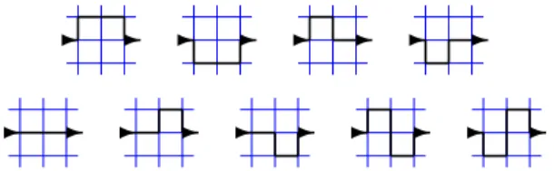
We now detail the case K = 3. There are nine walks which cross a 3 ⇥ 3 square from one side to the opposite side (see Figure 3):
- - -
-- - -
If we look at the rightmost walk of the first line, and consider it as a walk of length n in a 3k+1 ⇥ 3k+1
square, then each vertex on the walk can be seen as a walk in a 3k⇥ 3k square. More precisely, a walk of
length n is the concatenation of four walks which turn inside a 3k⇥ 3ksquare and one walk which crosses
a 3k⇥ 3k square from one side to the opposite side. So, if we denote by T
k(p)the number of F3 SAWs of
length p which turn inside a 3k⇥ 3ksquare, and by S
k(p)the number of F3SAWs of length p which cross
a 3k⇥ 3ksquare from one side to the opposite side, the number of walks which cross a 3k+1⇥ 3k+1square
like the rightmost walk of Figure 3 isPn1+...+n5=nSk(n1)· Tk(n2)· Tk(n3)· Tk(n4)· Tk(n5).
Using this method, we can get the total number of F3 SAWs of length n which cross a 3k+1 ⇥ 3k+1
square from one side to the opposite side: Sk+1(n) = X n1+n2+n3=n Sk(n1)· Sk(n2)· Sk(n3) + 2 X n1+...+n7=n Sk(n1)· Tk(n2)· Tk(n3)· Tk(n4)· Tk(n5)· Tk(n6)· Tk(n7) + 6 X n1+...+n5=n Sk(n1)· Tk(n2)· Tk(n3)· Tk(n4)· Tk(n5)
Using generating functions [9, 15] yields a more concise writing. If we set s(z) =Pn2NSk(n)zn, t(z) =
P
n2NTk(n)znand S(z) =Pn2NSk+1(n)zn, the equation above rewrites as:
S = s3+ 2st6+ 6st4 (1)
Without taking symmetries into account, there are eight walks who turn inside a 3 ⇥ 3 square (see Figure 4):
- 6 - 6 - 6 - 6 - 6 - 6 - 6 - 6
Figure 4: The SAWs turning inside a 3 ⇥ 3 square So, by setting T (z) =Pn2NTk+1(n)zn, we have:
T = t3+ t7+ s2t + 2s2t3+ 3s2t5 (2) For the square 5 ⇥ 5, we obtain the following:
S = s5+ 4s13t10+ 6s13t12+ 12s11t8+ 44s11t10+ 56s11t12+ 18s11t14+ 4s9t6+ 56s9t8+ 168s9t10+ 198s9t12+ 80s9t14+ 8s9t16+ 32s7t6+ 134s7t8+ 306s7t10+ 372s7t12+ 222s7t14+ 52s7t16+ 4s7t18+ 20s5t4+64s5t6+174s5t8+324s5t10+368s5t12+256s5t14+98s5t16+16s5t18+2s5t20+20s3t4+60s3t6+ 124s3t8+ 174s3t10+ 164s3t12+ 122s3t14+ 60s3t16+ 8s3t18+ 30st8+ 32st10+ 8st12+ 8st14+ 6st16 T = 2s14t9+ 2s14t11+ 4s12t7 + 14s12t9 + 14s12t11+ 6s12t13+ 16s10t7+ 46s10t9 + 76s10t11+ 52s10t13+ 12s10t15+ 14s8t5+ 54s8t7+ 171s8t9+ 278s8t11+ 228s8t13+ 68s8t15+ 6s8t17+ 4s6t3+ 26s6t5+ 123s6t7+ 306s6t9+ 483s6t11+ 406s6t13+ 168s6t15+ 26s6t17+ s4t + 4s4t3+ 22s4t5+ 86s4t7+ 239s4t9+ 370s4t11+ 337s4t13+ 194s4t15+ 62s4t17+ 14s4t19+ 2s4t21+ 4s2t3+ 10s2t5+ 19s2t7+ 54s2t9+ 85s2t11+ 86s2t13+ 45s2t15+ 18s2t17+ 6s2t19+ t5+ 3t9+ 5t13
Theoretically, for any odd K, it is possible to generate all the SAWs crossing a K ⇥ K square and then to derive from this the formulas for S and T . But practically, for K > 7, the generation of all the SAWs crossing a K ⇥ K square requires a prohibitively large amount of memory.
In [5, 4], A.J. Guttmann and others counted the SAWs crossing a square up to size 19 ⇥ 19 without generating them, using what they called the finite lattice method. It is easy to adapt their method to our purpose (generating the expressions for S and T ): instead of consider only the total number of SAW of length n between two points, we have to determine the number of SAWs of length n having k turns, for k in {0, . . . , n}. It is thus possible, after intensive computation, to obtain S and T for K up to 11.
From such a formula, it is possible to get the value for the connective constant µK. The radius of
convergence of the function C(z) = Pn2NcK(n)zn is equal to 1/µK. This radius of convergence can
be easily estimated by dichotomy: starting with an arbitrary value x for s and t, we reiterate (for K = 3) equations 1 and 2. If the result tends to 0, then |x| < 1/µK, and if it tends to the infinite, |x| > 1/µK. We
get the following values for µK:
F3: µ3⇡ 1.758; F5: µ5 ⇡ 2.035; F7: µ7 ⇡ 2.180; F9: µ9 ⇡ 2.269; F11: µ11⇡ 2.330;
4 Random Generation of Fractal SAW
It is very easy to randomly generate a K-fractal SAW: 1. Generate a random SAW in a K ⇥ K square.
2. Replace each vertex of the SAW by a random SAW in a K ⇥ K square. 3. Repeat step 2 until the SAW is long enough.
We can get drawings like those in Figure 5. With this generation method, we do not obtain an uniform
Figure 5: A 5-Fractal SAW of length 1434 and a 7-Fractal SAW of length 2745
distribution on the K-fractal SAW, since we can not fix the length of the SAW. But we have the following fact:
Let us Consider a randomly generated K-Fractal SAW for which Step 2 has been repeated p times. The distance between its two extremities is ⇠ Kp.
The shortest paths which go through a K ⇥ K square are of length K (we only consider paths which start at the middle of a side of a square and finish at the middle of another side). Let lS (resp. lT) be the
average length of the SAWs crossing (resp. turning into) a K ⇥ K square. If we consider only paths which turn on each squares, the average length of such paths for which Step 2 has been repeated p times is lp
S.
Similarly, the average length of randomly generated K-Fractal SAWs for which Step 2 has been repeated p times is in [min(lS, lT)p, max(lS, lT)p]. We have Kp = ((K0)p)logK0K and logK0K < 1for K0 = lS or
K0 = lT, so we conjecture the following:
The critical exponent ⌫ for the K-Fractal SAW is < 1, i.e. the average distance between the two extrem-ities of a K-Fractal SAW of length n is ⇡ n⌫, with ⌫ < 1.
We conjecture that this is true for the uniform distribution. Actually, the random generation process can be seen as a decision tree. At each level, one uniformly choose a SAW in a K ⇥ K square. But a long SAW has more (and longer) descendants than a short one. So, with the distribution got with the generation process, the short paths are overrepresented.
5 Variants
One can imagine many variants of Fractal SAW. We present some of them in this section. The first way of defining variants consists in taking other building blocks that the square.
For example, the same definition can be applied to the lattice Zd for any d 2, with hypercubes
instead of squares and we cn use the same technique to compute the connective constant. For instance, for 3 dimensional cubes 3 ⇥ 3 ⇥ 3, we have µ = 2.799.
It is also possible to use rectangles instead of squares, but one has to consider three types of SAWs crossing a rectangle: those which turn inside the rectangle, those which cross from a small side to the other one and those which cross from a long side to the other one.
We can also forbid some squares (of size Kp⇥ Kp) inside squares of size Kp+1⇥ Kp+1. For instance,
if we forbid the central node in a 3 ⇥ 3 square, we can get a Fractal SAW on the Sierpi´nski carpet [14] (see Figure 6). For such SAWs, we have:
S = 2st4
T = t3+ s2t5
And thus µ = 1.207
One can add some restrictive conditions, in order to obtain a family of SAWs which is easier to study. For instance, if we force to a Fractal SAW to always turn inside a square (of any size, including the nodes), we get a Sinuous SAW [3] for which only one parameter is necessary for counting. We get:
K = 3: T = t3+ t7
K = 5: T = 3t9+ 5t13+ t5
K = 7: T = 6t11+ 28t19+ t7+ 34t23+ 15t15+ 23t27+ 5t31
. . .
Figure 6: A 3-Fractal SAW of length 4880 on the Sierpi´nski Carpet K µ 3 1.210 5 1.288 7 1.335 9 1.376 K µ 11 1.405 13 1.427 15 1.444 17 1.458
Figure 7: The connective constant µ for Sinuous SAWs
It is also possible to require the walk, inside a square, to belong to a well known family, as the prudent SAWs [7] or the up-side SAWs [16]. It is this possible to count the SAWs crossing a square without enu-merate them, thus with no intensive computations. It is so possible to get the connective constants for this kind of SAWs for much larger squares that for the basic family. We will detail the up-side SAWs.
An up-side SAW is a SAW on the square lattice which never goes down. If a K-Fractal SAW is, up to a rotation, a up-side SAW inside each square (the smaller squares are considered as points), we say that it is a K-Fractal-UpSide SAW (see Figure 8). Equivalently, a SAW is Fractal-Upside if, inside every square, there is a forbidden direction (if the walk enters the square on the West side and goes out through the opposite side, the forbidden direction is West; if the walk enters the square on the West side and goes out through the South side, the forbidden direction can be West or North). One can notice that a K-Fractal-UpSide SAW is generally not Up-Side. The advantage of such Fractal SAW is that it is possible to get the number of SAWs into a K ⇥ K square without intensive computations:
There are two types of Up-Side SAWs: the ones whose last move was a North move, and the ones whose last move was an East or a West move. When last move is North, next move can be North, East or West; when last move is East (resp. West), next move can be North or East (resp. West). Since we consider moves inside a square, we have to take into account the “remaining place” into the square (see Figure 9). If we call U (d, r, s, t)(resp H(d, r, s, t)) the number of K-Fractal-UpSide SAWs starting at the middle of the South side, ending at distance d from the North side and r from the East side, whose last move is North (resp. East), with s straights and t turns, we have:
-X ⇠
Figure 8: A 5-Fractal-UpSide SAW 6
? d
-K r r- K -r r
-Figure 9: The parameters to be considered to count K-Fractal-UpSide SAWs U (d, r, s, t) = U (d + 1, r, s 1, t) + H(d + 1, r, s, t 1) + H(d + 1, K r + 1, s, t 1) H(d, r, s, t) = U (d, r + 1, s, t 1) + H(d, r + 1, s 1, r)
H(K, (K + 1)/2, 0, 0) = 1
In addition, if we call S(s, t) the number of K-Fractal-UpSide SAWs with s straights and t turns crossing a K⇥ K square from one side to the opposite one, and T (s, t) the number of K-Fractal-UpSide SAWs with sstraights and t turns turning into a square, we have:
S(s, t) = U (0, (K + 1)/2, s, t)
T (s, t) = 2· H((K + 1)/2, 0, s, t) C(s, t)
The 2 factor for T (s, t) is because there are two (symmetrical) types of K-Fractals-UpSide SAWs turning into a square (see Figure 10, left and middle); but SAWs which contains only North and East moves (see Figure 10 , right) belong to the two categories. So we remove their number (that we call C(s, t)). It is thus
- -
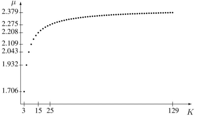
-Figure 10: Three K-Fractal-UpSide SAWs turning into a square possible to obtain the values for the connective constants µ shown in Figure 11.
q q qqq qqqqqqqq qqqqqqqqqqqqqqqqqqqqqqqqqqqqqqqqqqqqqqqqqqqqqqqqqqq -K 129 2.379 3 1.706 15 2.208 25 2.275 1.932 2.043 2.109 6 µ
Figure 11: The connective constant µ for K-Fractal-UpSide SAWs
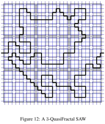
The last way of defining variants of fractal SAWs consists in loosen the definition. We will remove Condition 11. So we now consider SAWs which always enter into (or go out of) a square through the middle
of a side (see Figure 12). These SAWs can come back into an already visited square. We cell such SAWs K-QuasiFractal SAWs and we denote by QFKthe sets of K-QuasiFractal SAWs. As for K-Fractal SAWs,
we have:
Property 3. limK!1QFK is the set of all SAWs.
For every K, QFKhas a connective constant.
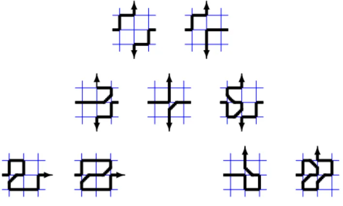
Similarly, in order to count K-QuasiFractal SAWs, we only have to enumerate walks in a K ⇥K square. As for K-Fractal SAWs, we will count directed SAWs, but we have now to consider three types of walks (see Figure 13):
• The ones who go from one side of a square to the opposite side. • The ones which turn inside a square.
• The ones which “crosses” in a square, i.e. which are made of two independent SAWs. We have to notice that this type of SAW does not concern vertices and that, since we count directed SAWs, crossing configurations as the one of Figure 14 are impossible.
In addition, for squares of size greater than K2⇥ K2, there are more walks crossing square from one
side to the opposite one (or turning into a square) than for K-Fractal-SAW (see Figure 15), and there are 19 such walks which go from one side of a 3 ⇥ 3 square to the opposite side, 18 which turn into a 3 ⇥ 3 square and 22 which cross into a 3 ⇥ 3 square. For 3-QuasiFractal SAWs, we get the following formula:
S = s3+ 6st4+ 4st4c2+ 2st6+ 2s3t4c2+ 4st6c
1It is not possible to remove Condition 2. The main tool that we used for counting Fractal SAWs (or their variants) was that a Kp
⇥ Kpsquare inside a Kp+1
⇥ Kp+1square is like a vertex inside a K ⇥ K square. Using this tool implies that the squares are all independent (what “happens” inside a square does not depend on what happens in another one). Removing Condition 2 would add dependency between squares of different sizes: for instance, if a walk enter a square at a corner, it enters squares of all the smaller sizes by this corner.
Figure 12: A 3-QuasiFractal SAW
-6 6
?
Figure 13: The three types of walks to be considered for counting K-QuasiFractal SAW T = s2t + t3+ 3t5c3+ s2t3c + 3s2t5+ 2s2t3+ t7+ 2s2t5c2+ 2s2t5c + 2t5c
C = s4c + 2s2t4+ 8t4c5+ 4s2t4c + 6t6c2+ t6
where c(z) =Pn2NCk(n)zn, C(z) = Pn2NCk+1(n)znand Ck(n)is the number of walks which cross
into a 3k ⇥ 3k square. Using the finite lattice method, it is possible to compute similar formula for
5-QuasiFractal SAWs and 7-5-QuasiFractal SAWs, from which we can get the values of the connective constant µin Figure 16.
K µ
3 1.862 5 2.155 7 2.312
-6
Figure 14: An impossible walk for K-QuasiFractal SAW
- - 6 6 ? 6 ? 6 ? 6 ? ? 6 6
Figure 15: Examples of paths to be considered for 3-QuasiFractal-SAWs but not for 3-Fractal-SAWs. Only the cases in the top line occur in 3 ⇥ 3 squares. The other cases occur only in greater squares. A node in a 3p+1⇥ 3p+1square like the central one in the middle drawing of the second line corresponds (up to
symmetries and rotations) to a path in a 3p⇥ 3psquare like the ones in the two upper lines.
References
[1] A. Bacher & M. Bousquet-M´elou, Weakly Directed Self-Avoiding Walks, J. Combin. Theory Ser. A, 118 (2011), 2365-2391.
[2] M. Bousquet-M´elou, Families of Prudent Self-Avoiding Walks, J. Combin. Theory Ser. A,117 (2010), 313-344.
[3] M. Bousquet-M´elou, Les Chemins Auto- ´Evitant de Pascal, Personnal communication (2010). [4] M. Bousquet-M´elou, A.J. Guttmann & I. Jensen, Self-Avoiding Walks Crossing a Square, J. of Phys.
A38 (2005), 9159-9181.
[5] A.R. Conway, I.G. Enting & A.J. Guttmann, Algebraic Techniques for Enumerating Self-Avoiding Walks on the Square Lattice, J. of Phys. A26 (1993), 1519-1534.
[6] J.C. Dethridge & A.J. Guttmann, Prudent Self-Avoiding Walks, Entropy8 (2008), 283-294. [7] E. Duchi, On Some Classes of Prudent Walks, FPSAC’05, Taormina, 2005.
[8] H. Duminil-Copin & S. Smirnov, The Connective Constant of the Honeycomb Lattice Equalsp 2 +p2, Annals of Mathematics175(3) (2012), 1653-1665.
[10] P.J. Flory, The Configuration of a Real Polymer Chain, J. Chem. Phys.17 (1949), 303-310.
[11] P.G. de Gennes, Exponents for the Excluded Volume Problem as Derived by the Wilson Method, Phys. Lett. A38 (1972), 339-340.
[12] I. Jensen & A.J. Guttmann, Self-Avoiding Polygons on the Square Lattice, J. Phys. A. 32 (1999), 4867-4876.
[13] N. Madras & G. Slade, The Self-Avoiding Walk, Birkh¨auser, 1993.
[14] W. Sierpi´nski, Sur une courbe cantorienne qui contient une image biunivoque et continue de toute courbe donn´ee, C.R.A.S. Paris162 (1916), 629-632.
[15] H.S. Wilf, Generatingfunctionology, Academic Press, 1994.
[16] L.K. Williams, Enumerating Up-Side Self-Avoiding Walks on Integer lattices, The Electronic Journal of Combinatorics3, #R31.