Contextual language understanding Thoughts on Machine Learning in Natural Language Processing

(1)

HAL Id: tel-02470185

https://hal-amu.archives-ouvertes.fr/tel-02470185

Submitted on 7 Feb 2020

HAL is a multi-disciplinary open access

archive for the deposit and dissemination of

sci-entific research documents, whether they are

pub-lished or not. The documents may come from

teaching and research institutions in France or

abroad, or from public or private research centers.

L’archive ouverte pluridisciplinaire HAL, est

destinée au dépôt et à la diffusion de documents

scientifiques de niveau recherche, publiés ou non,

émanant des établissements d’enseignement et de

recherche français ou étrangers, des laboratoires

publics ou privés.

Machine Learning in Natural Language Processing

Benoit Favre

To cite this version:

Benoit Favre. Contextual language understanding Thoughts on Machine Learning in Natural

Lan-guage Processing. Computation and LanLan-guage [cs.CL]. Aix-Marseille Universite, 2019. �tel-02470185�

(2)

Thoughts on Machine Learning in Natural Language Processing

Benoit Favre

January 1, 2020

(3)

(4)

Foreword

This document is a habilitation à diriger des recherches (HDR) thesis. It is organized in two parts: The first part presents a reflection on my work and the state of the Natural Language Processing community; The second part is an overview of my activity, including a detailed CV, a summary of the work of the PhD students I contributed to advising, and a list of my personal publications. Self-citations are postfixed with† and listed in Chapter 9, while external references are listed in the bibliography at the end of the document. Each contribution chapter ends with a section listing PhD student work related to that chapter.

(5)

(6)

Abstract

Natural language is pervasive in a society of information and communication. Processing it auto-matically, be it in the form of analysis or generation, is at the center of many artificial intelligence applications. In the last decades, the natural language processing (NLP) community has slowly adopted machine learning, and in particular more recently deep learning, as a major component of its research methodology. NLP tasks are typically expressed as structured classification problems, for which sys-tems can be devised by finding parameters that minimize a cost function on a previously hand-labeled training corpus.

This document explores the current state of the research questions addressed by the NLP com-munity through three interwinded challenges: taming modeling assumptions, ensuring generalization properties and dispensing adequate methodology.

Modeling assumptions are often seen from a statistical point of view, such as the assumption that training samples shall be independently distributed, yet NLP assumes other kinds of dependency as-sumptions which impact system performance. Input representations, and in particular the scope of input features used to characterize a decision, may need to be reconsidered when processing rich lin-guistic phenomena. Structured predictions for which decisions are interdependent are tackled through a compromise between rich decoding schemes with low modeling power, and suboptimal decoding with richer models. Linguistic descriptions have lead to modular approaches resulting in processing chains hindered by cascading errors, an approach questioned by recent end-to-end and multitask training.

The second challenge is performance generalization, meaning that systems shall not collapse under conditions differing from the training distribution. Generalizing NLP systems across genres, such as from news to social media, and modality, from text to speech, requires accounting for the distributional and representational shift between them. In addition, recent development of common annotation schemes over a range of languages, and the resulting availability of multilingual training data allows to explore creating systems that can process novel languages for which they have not received full supervision.

The third challenge is methodological, exemplified through problems with shared tasks and lack of user involvement in current evaluation metrics. Shared tasks, a tool used to foster progress through independent evaluation of systems developed by competing scientific institutions, are both beneficial and detrimental due to over-engineering and bias effects. Besides shared tasks, the loss functions encouraged by machine learning for training NLP systems are often generic and do not account for the context in which they are used. Developing user-oriented evaluations is a research direction for improving this involvement.

(7)

(8)

Contextual Language

Understanding

(11)

(12)

Chapter 1

Introduction

In order to make machines significantly easier to use, it has been proposed (to try) to design machines that we could instruct in our native tongues. This would, admittedly, make the machines much more complicated, but, it was argued, by letting the machine carry a larger share of the burden, life would become easier for us.

Edsger W. Dijkstra, 1979 Natural Language Processing (NLP) is a field of computer science which aims at studying how human language in all its forms can be processed and generated by computers. Originating from a multidisciplinary community, it draws from the fields of mathematics, philosophy of language, linguis-tics, psycholinguislinguis-tics, cognitive sciences, social sciences, neuroscience, in order to model and simulate human behavior regarding natural language.

A definition of the word language, given in (Crystal et al.2018), could be “a system of conventional

spoken, manual, or written symbols by means of which human beings, as members of a social group and participants in its culture, express themselves. The functions of language include communica-tion, the expression of identity, play, imaginative expression, and emotional release.” This definition

actually restricts itself to natural language, by opposition to formal languages which are mathemat-ical constructs made of sequences of abstract objects with interesting regularities, in which fall for instance programming languages. Even though formal languages are often used to describe some as-pects of natural languages, the ‘natural’ modifier has been included because of the complexity of the observed phenomenon of human-human communication that may be beyond the reach of simple formal languages. The debate between formalists and naturalists probably originated in Noam Chomsky’s interest for the source of the phenomenon of language in the mind (embodied by the study of formal languages) and relative lack of interest for how this phenomenon translates into actual linguistic in-stances, corrupted by actuators and communication channel issues. Yet, corpus-based linguistics and the ensuing empirical evaluation of natural language processing systems have led to very successful applications that changed our everyday life, and that would probably not have been possible if the community did not focus on natural language at some point.

The previously mentioned definition of language also imposes interesting restrictions on the kind of symbolic systems used for conveying language, and the fact that language is a human-centric concept. While spoken language is the means of choice for human communication and the first language a baby learns, written language has been the favorite durable means of communication because it could be painted, written, printed, and sign language even if most developed in disabled communities, is a recognized complement to spoken language and one of the first languages infants can learn. A first

(13)

question entailed by this restriction is whether language can be expressed in other modalities. For instance, music is often recognized to have a lot of properties of language (Rohrmeier et al.2015), and therefore should it be considered as a natural language? Another question is whether the symbols upon which language relies need to be discrete or could be of another form. The space of colors is inherently continuous, and language has trouble mapping it with symbols; paralinguistic information such as emotions also do not map well to a symbolic space; sign language has many non-symbolic constructs based on location or intensity of gestures. Maybe the underlying question is whether thinking is symbolic and, if not, how it maps to a symbolic language (Lupyan2016). The second restriction is the limitation to human communication. It has been shown multiple times that animals use some form of language that have a lot in common with human language, and it is also interesting to question whether natural language processing should be limited to human language (and there are several current efforts to build dog-human translation devices, with various degrees of success).

The general public perception of natural language processing is that since language manipulation is so easy for humans, it should be as straightforward for machines. Automatic speech recognition, the generation of a transcript from what was said in an audio recording, is a typical example of an intuitively easy yet extremely difficult task. The first problem is the recognition of phonemes from the acoustic signal. Phonemes are the basic unit of sound that can be produced by the vocal conduct, such as vowels (sustained frequencies produced by driving air through the vocal folds) or consonants (produced for example by fast tongue and lip movements). Recognizing phonemes is challenging because different morphologies of the vocal conduct lead to speaker-level variability of the frequencies and timing that characterize a phoneme. It is also challenging because the vocal conduct is a continuously moving organ which results in slow transitions between the stable states of phonemes. In addition to those challenges, the acoustic channel (reverberation, distance to the microphone, type of microphone, presence of other sources of noise) may be corrupted leading to uncertainties in the recognition process. Even if the phoneme sequence were easy to reconstruct, mapping phonemes to lexical units is difficult because of ambiguity. Given a phoneme sequence, there are typically hundred thousand sequences of words that map to that sequence among which most are nonsense but some make perfect sense out of context (a good source of puns). A speech recognition system has to guess the actual sequence, which often implies understanding the intent of the original speaker. Automatically understanding such natural language, called Natural Language Understanding or NLU, is also difficult because of ambiguity (a single word might have multiple senses), because of the use of references which require to account for a broad context (for instance relying on general knowledge), and because the target of what “understanding” means (and in general what semantics is) is ill-defined and often an open research problem.

Natural language processing includes some of the most difficult problems of the field of artificial intelligence because they often require world knowledge and general reasoning (therefore, it is listed as one of the IA-complete problems, possibly requiring general Artificial Intelligence), yet many success-ful applications have been striving over the years. These applications rely on mimicking how humans manipulate language in a specific context or domain instead of completely simulating an intelligent system. General purpose dialog agents, also known as “chatbots”, are a good example of how humans can be deceived in thinking that they are talking to an intelligent machine. The Turing test, long thought as a good test of achieving artificial intelligence, consists in blindly matching human judges with dialog agents and other humans, and measuring whether the judges can discriminate between humans and computer programs. The ELIZA chatbot (Weizenbaum1976) or contestants to the Loeb-ner Prize competition (Stephens2004) are dialog systems which rely on conversational tricks in order to evade difficult questions (such as invoking boredom, switching topics, etc.) Machine Translation is another example which uses recurrent statistical properties of aligned corpora across languages in order to mash-up good-quality translations. One fundamental question of NLP is whether we should continue to make mimicries, in the same way the aeronautics community has built planes instead of simulating bird flight, or if we can overcome the difficulties of simulating cognitive functions of the brain.

While early natural language processing systems relied on formal models (the introspective ap-proach), the community has slowly evolved towards using statistical models of language to eventually

(14)

relying on machine learning for a broad range of NLP tasks. This evolution probably began with the introduction of corpora of naturally occurring language phenomena for evaluating the quality of NLP systems. This was a step towards more ecological evaluation of language technology. As corpus size grew, it started to be possible to tune system hyper-parameters to maximize performance, and finally to use a subset of the annotated data to train machine learning algorithms. Machine learning consists in creating computer programs that can learn from experience without being explicitly designed to solve a particular task. The inference problem is often formalized as generating the output (class label, symbolic structure or set of real values) from a parametrizable function of the input (features extracted from observations), while the learning problem consists in finding the parameters of the function that best generate the correct labeling of a corpus. The approach developed in the NLP community by first replacing hand-designed rule-based systems with automatically mined rules from a superset of possible rules, which made the success, for example, of the Brill part-of-speech tagger (Brill 1992). Later, researchers developed statistical approaches leveraging independence assumptions to decompose joint probabilistic models of the labels to predict and observations, and computed the probability of events through a frequentist maximum likelihood estimation of discrete distributions. These approaches lead to success in automatic speech recognition (Huang et al.1990), language modeling or machine trans-lation (Koehn 2009). Another landmark approach was maximum entropy (Berger et al. 1996) and conditional random fields (Lafferty et al.2001) which extend the frequentist statistical approach to a log-linear modeling of distributions decomposed over features of the input. The NLP community then followed more closely the advances in the machine learning community. More classes of models have been made possible to explore by formalizing the learning problem as a loss function minimization problem, and directly minimizing the end-task errors (such as approximations of BLEU in machine translation). While most prominent models were linear, nonlinear models have long been explored with decision trees, support vector machines or neural networks. Finally, recent advances in deep learning have promoted neural networks to the dominant approach for a lot of NLP problems, such as speech recognition, machine translation, etc. In major conferences and journals of the domain (Com-putational Linguistics, ACL, EMNLP, EACL, NAACL, COLING, etc.), the percentage of papers with titles related to machine learning has tripled from 2010 to 2018, going from around 10% to more than 30% (lower bound on actual topical content; see Table1.1). Clearly, machine learning is establishing itself as a very strong component of the field. This observation makes one wonder whether this trend will last, or whether machine learning will eventually fade and be replaced.

Year Matches Total %

1965-2009 1,494 20,671 7.2 2010 269 2,666 10.1 2011 207 1,856 11.2 2012 279 3,047 9.2 2013 298 2,540 11.7 2014 371 3,297 11.3 2015 464 2,587 17.9 2016 806 3,722 21.7 2017 970 3,144 30.9 2018 1,468 4,335 33.9 mid-2019 379 1,120 33.8

Table 1.1: Number of article titles of the major conferences and journals of the domain indexed in the ACL Anthology (CL, ACL, EMNLP, EACL, NAACL, COLING, etc.) that match typical machine learning words (neural, learning, deep, training, embedding, network, end-to-end, attention,

lstm, ensemble, adversarial, bayesian, supervised, margin, support, loss) from 1965 to mid-2019 with

of focus on recent years. Data collected fromhttps://aclanthology.info.

(15)

development, model choice and parameter tuning, evaluation protocols and shared tasks) is favored by the community for the following reasons. First, it is considered as a step towards ecological evaluation through the use of collected naturally occurring language data. It also helps building a repeatable experimental setup because machine learning algorithms, trained with the same corpus and given the same initial parameters, lead to the same performance results on the test set. One advantage of machine learning that is a dividing argument in the community is that associated models are often linguistic-theory neural and by being able to learn relevant features from the data, require less linguistic expertise on the target problems. This aspect also allows to capture regularities that are not apparent in the data, and therefore often yields superior performance in scientific competitions. Another benefit is that machine learning models can often account for very large datasets and are relatively eﬀicient in terms of processing. An additional reason is that some aspects of machine learning imitate the learning process of the brain, allowing computers to learn language in the same way children learn language. This last reason is debatable since it is not settled how much of the implementation of language in the brain is the result of evolution, and how much is the result of social interaction.

While machine learning may seem like a definitive answer to a very broad range of problems, it also exhibits some limitations which have been recognized by various communities. The main disadvantage is that machine learning requires much more supervision than humans for being able to obtain reasonable performance (and even sometimes super-human performance) in solving a particular class of problems. There have been many efforts to increase data eﬀiciency, such as active learning techniques (Settles2012) which consist in iteratively training a system and selecting which examples to annotate in order to maximize the performance gain of the system. Another trend of research is that of meta-learning in which machine learning systems are faced with numerous different tasks so that they get a chance at capturing faster the specifics of a novel task (Finn et al. 2017). In the computer vision community, it has been shown multiple times that it is easy to add noise to images that perceptually belong to a category unambiguously while a trained system gives a different category with very high confidence. Attacking machine learning systems with adversarial examples is an old topic as evidenced in the speaker verification community with voice transformations that allow spoofing an identity (Matrouf et al.2006), or by more recent techniques for building physical objects that can consistently fool machine learning systems while being recognized by humans (Kurakin et al.2016). In order to contain the effects of such attacks, but also required by certain application domains such as medicine, recent efforts in machine learning have focused on making systems which are interpretable at the model level (what did the model learn, how did it learn?) and at the decision level (why did the mode make a given decision?). It is often stated that deep neural networks are not interpretable, but one can remark that linear models are not much more interpretable than their deeper peers (Lipton

2016).

Given the attraction of the NLP community for machine learning in face of the benefits and drawbacks it carries, it is reasonable to question whether those specificities are important for the NLP field, and try to shape what compromises the community is making by focusing on a single approach. This document presents a set of reflections based on my experience at the saddle point between the fields of natural language processing and machine learning, and illustrated and supported by arguments based on the research I have conduced since my MSc thesis. Its aim is to introduce elements that can help us move towards answering the following questions:

• What is the impact of assumptions typically associated with machine learning on current NLP research?

• Are models trained through machine learning able to generalize well on natural language pro-cessing tasks?

• What are the limits of methodological practices in the natural language processing community in the context of machine learning?

• On what problems should the NLP community focus now that reliance on machine learning has matured?

(16)

This document does not give a definitive answer to those questions. But it shows directions which might lead to a better understanding of a range of NLP problems. Those directions are based on the idea of extending the context in which problems are tackled, by pushing the envelope of formalization, modeling, implementation and methodology associated with them. This approach is fundamental to

Contextual Language Understanding.

This part of the document is organized as follows. Chapter 2 gives a broad overview of major natural language processing techniques with a focus on recent deep learning approaches. Chapter3is an attempt at measuring the impact of assumptions on NLP system performance. Chapter4 tries to determine up to what point generalization is limited in current NLP approaches. Chapter5 addresses some of the methodological concerns with current practices in empirical research in the community. The last chapter of this part gives a general conclusion and lists a few prospects in the field.

(17)

(18)

Chapter 2

Modern Natural Language

Processing

Many introductions to natural language processing, encompassing historical or recent approaches, can be found in the literature. The objective of this chapter is not to build a comprehensive survey of existing problems and methods but rather to focus on select landmarks that are relevant to the next chapters. In particular, it only covers a few supervised machine learning techniques popular within the community for a large number of NLP tasks. For a more in-depth approach of NLP, the reader may refer to (Jelinek1997; Manning et al.1999; Martin et al.2009; Koehn2009; Goldberg2016; Deng et al.2018).

This chapter first covers the dominating methodological approach to building NLP systems based on empirical evaluation of their performance on “language-in-the-wild” corpora. Then, it outlines a broad family of NLP tasks and reviews machine learning approaches that can be exploited to tackle them.

2.1 An Empirical Approach

Empirical evaluation has become the workhorse of the natural language processing community. In terms of methodology, the main problems that need to be addressed are reproducibility (research results can be replicated), and representativeness (the experimental setting is realistic). To address both, researchers have been resorting to the notion of corpus, a set of language samples collected from actual interactions or sources, which stand as representative of the NLP problem being addressed. Corpora can be made accessible for others to replicate results, and can be collected from a variety of settings to ensure realism.

The typical approach for creating an NLP system consists in the following loop:

1. define the task, be it part-of-speech tagging, named entity recognition, machine translation, or summarization;

2. gather corpora that encompasses a range of sources, genres, styles to be representative of the applications you have in mind;

3. write a precise and coherent annotation guide, and define a meaningful evaluation criterion; 4. annotate the corpora with task labels using informed or naive annotators to build a gold

stan-dard;

5. create a system that will predict labels from raw data; 17

(19)

6. evaluate the system output on held-out data;

7. loop to step (1) to refine the approach – only a subset of steps might be refined (for instance, it is common to alternate between improving a system and evaluating it).

This loop, which could be called TCGASE (for Task, Corpus, Guide, Annotation, System, Evalua-tion), is essential not only to current NLP research, but also to system engineering in the industry as quality control. It is suitable for creating machine-learning based systems as it provides an environ-ment with labeled data and a criterion to optimize for. In the following sections, we detail a bit more the notions of task, system and evaluation metrics.

2.2 Tasks

Traditionally, NLP tasks are organized according to the analysis-synthesis dichotomy, as well as the means-and-end dichotomy which considers intrinsic tasks (which are steps towards an end) and ex-trinsic tasks (which can be involved in end-user applications). However, the boundary between those categories is very loose as the same models can often be used for analysis and synthesis, and a lot of intrinsic tasks can be exposed in applications.

Another way of looking at NLP tasks is according to processing levels: meta, syntactic, semantic, discourse and pragmatic levels. Automatic processing at those levels is typically performed sequentially, from the lower to the higher level. A non-exhaustive list of tasks could be described as follows.

• The Document level operates on meta-descriptors of the linguistic content:

– Language and code identification and segmentation: finding what language the current

doc-ument contains, some docdoc-uments containing multiple languages, or sequences of words using different writing systems, such as the inclusion of English words in Chinese, or mathematical symbols in an article;

– Author identification and trait classification: characterizing the style of an author to devise

her identity or traits such as social category, age, etc.;

– Document structure analysis: determining where structural elements such as section

head-ers, paragraphs, lists, figures, etc. are.

• The Syntactic level corresponds to structural elements that are linked to the function of lin-guistic elements:

– Sentence splitting, punctuation prediction: finding where sentences start and end, which

can be diﬀicult in spontaneous spoken or textual content;

– Word segmentation, tokenization, multiword expression detection: identifying words and

associated lemmas in the stream of characters which might not be separated by spaces or punctuation such as in Sino-Tibetan languages;

– Part-of-speech tagging, morphological analysis: determining the syntactic category of words,

as well as traits such as gender or number which can be determined from sequences of characters within words;

– Syntactic chunking and parsing: finding the latent structure that links words together

outlining the function of groups of words under a grammar theory. • The Semantic level aims at analyzing the meaning of linguistic constructs:

– Named entity recognition, linking: identifying sequences of words which correspond to

real-world entities and matching them in a database of existing entities;

– Word-sense disambiguation: recognizing the meaning of each lexical unit among a catalog

(20)

– Topic classification and segmentation: finding the topic or hierarchy of topic segments of a

document;

– Semantic parsing: constructing the latent structure of the sense of a sentence from the

meaning of individual words according to one of the semantic representation theory. • The Discourse level drives how discourse and interaction are organized

– Coreference resolution: resolving pronouns and references to aforementioned entities or

external entities;

– Dialogic parsing: analyzing the construction of a dialog or a multiparticipant conversation

in terms of dialog acts, question-answer pairs, etc.;

– Discourse parsing: determining how arguments are constructed and related.

• The Pragmatic level consists in the integration of meaning units in the context in which they are produced, often with an applicative end in mind.

– Sentiment analysis and opinion mining: determine the stance or emotional state of an

author, speaker or character regarding a topic;

– Knowledge representation: build an ontology or formal representation of knowledge acquired

from a text or during a communication effort;

– Reasoning / integration: reason about what to do next given the current state of system

and linguistic input (dialog systems, robots, etc.).

It is apparent that some of those task do not completely fit the category they are attached to, and that some may benefit from the output of a number of other tasks. This description towards the analysis side of NLP also holds (in reverse level order) for the generative side which aims at producing linguistic constructs given abstract representations.

Natural language processing has generated a number of applications that span the whole industry of human-human and human-machine interactions, such as machine translation, summarization, speech recognition or dialog systems. Those applications might be treated as compositions of finer-grained NLP tasks, or tasks of their own.

Most of those tasks can be cast as one of five problems:

• Labeling: predict an output label from a set of possible labels (a classification task), often extended to sequence or tree labeling because the label for one element depends on neighboring elements. Word sense disambiguation or part-of-speech tagging belong to that category.

• Segmentation: predict segment boundaries for the input, as a partition of disjoint, possibly overlapping segments. Syntactic chunking or named entity recognition are instances of this task. A non-overlapping segmentation task can be cast as a sequence labeling problem by using the popular begin-inside-outside (BIO) encoding which appends a B to the first item of a segment, an I to all items inside it and an O for items which are not in a segment1_.

• Regression: predict a value in a continuous space, such as for sentiment valency assessment, predicting the quantity of silence required for a dialog system to take the floor, speech synthesis (generation of a sequence of audio samples), or predicting customer satisfaction on Likert scale. When the nature of the target is not natively continuous, the problem is often mapped to (ordered) labeling.

• Relation detection: predict that two elements are in relation, and label that relation. Depen-dency parsing is cast as relation detection, but so can be coreference resolution. Some constraints can be added to the task as in dependency parsing where a word can only have one governor, which ensures that the created structure is a tree.

1_{There exist a range of representations of segments as word-level classification tasks (Konkol et al.}₂₀₁₅_{) and explicit}

(21)

• Generation: predict a label which decomposes as a sequence of items (generally words). It is the case of summarization or machine translation for which a sequence of words must be generated. The advent of deep learning has greatly extended the expressivity of machine learning systems, blurring this categorization2_.

2.3 Systems

Given this description of natural language tasks, it would be interesting to be able to reuse similar methods for dealing with different problems. The mainstream approach is to use machine learning to solve those problems.

NLP problems are often treated as classification of an input x ∈ X as a label y ∈ Y where X and Y are respectively the set of all possible inputs and labels. When X or Y are large, x and y

are decomposed in smaller units, such as words and part-of-speech tags of a sentence. The inference problem consists in predicting y given x, with a parameterized function fθ.

ˆ

y = argmax

y∈Y

fθ(x) (2.1)

Training consists in finding the parameters θ that minimize an empirical loss on never seen data (for example the number of mislabeled instances), which is approximated by minimizing a loss function

L on a training corpusC, which is called empirical risk minimization (ERM).

ˆ θ = argmin θ ∑ (x,y)_∈C L(y, fθ(x)) (2.2)

In the following sections, we overview a few “shallow” machine learning models and “deep” neural networks that are often used in NLP systems.

2.3.1 Standard models

Perceptron The perceptron algorithm is one of the most straightforward linear model for machine

learning. If x is a feature vector, W a weight matrix of size the number of features times the number of possible labels, y is a score vector with a value for each label (the highest scoring label being the predicted one). Prediction under that model is performed as:

y = W x (2.3)

Training is achieved by stochastic gradient descent by repeatedly sampling examples from the training set, performing prediction, and adjusting the weights according to whether the correct label was predicted or not. The gradient is discretized so that−1 is added to the weights of the incorrectly

highest scoring label, and 1 is added to the weights of the gold label that should have been predicted, in a maximum margin fashion. A very good extension is the averaged perceptron which consists in saving the weight matrix after each update, and eventually averaging all the weight matrices to produce the final model (Collins2002). It can be computed eﬀiciently by observing that the average model can be factorized according to each of the updates.

Structured prediction problems can be tackled by decomposing y in substructures and using an inference procedure, such as the Viterbi Algorithm for chains of factors, and then adjust the weights of the features linked to the substructures. The size of W depends on the number of features times the number of values the substructures can take (for a bigram tagger, they would be the number of possible tag bigrams) which tends to grow quickly in practice. Sparse representations are often used for both x and W .

2_{Systems can be set up to solve hybrids of those problems although the various losses they are trained for can be}

(22)

The perceptron algorithm has been very popular in the NLP community for its simplicity and speed, while achieving very good results in tagging and parsing tasks at a fraction of the cost of other models (Collins2002; McDonald et al.2005a). A number of variants of the training procedure have been proposed, such as Mira (Crammer et al. 2006) or Adagrad (Singer 2010), without leading to systematic improvements compared to the averaged perceptron.

Maximum entropy and conditional random fields Maximum entropy models are log-linear probability models which can be expressed as:

pθ(y|x) = 1 Z(x)exp ( ∑ k θkfk(x, y) ) (2.4) Z(x) = ∑ y′∈Y exp ( ∑ k θkfk(x, y′) ) (2.5) where θ is a vector of trainable parameters and f (x, y) is a binary feature vector for the label y of x.

Z(x) is a normalization factor which makes the probabilities over labels y sum to 1.

Log-linear models can be trained by maximizing the log likelihood of the training data, with an optional regularization penalty (Lreg(θ), with λ regulating the quantity of regularization, determined

on a development set).

L(θ) =∑

i

log pθ(y(i)|x(i)) (2.6)

Lreg(θ) =

∑

i

log pθ(y(i)|x(i))−

λ

2 ∑

j

θ2j (2.7)

L(θ) (and Lreg(θ)) is convex and can be maximized with any off-the-shelf algorithms such as gradient

ascent or LBFGS (Liu et al.1989). Closed-form derivation of the gradients ofL with respect to θ can

be found in (Collins2005).

Conditional Random Fields (CRF) are maximum entropy models applied to labels y decomposable over a graph of factors. The basic idea is that an instance consists in a set of slots T which have to be labeled with atomic labels yt∈ YT so that y ={yt}T. Then, we can consider GT a graph over T

and factors as connected components, or cliques, of GT. Intuitively, the factors are subsets of atomic

predictions in T that represent dependent phenomena. Given that, a CRF is a log-linear model where binary features are extracted for each factor, and associated with trainable weights. Since cliques may share slots, the inference problem (finding the highest scoring labeling of the graph) must make sure that factors agree on the atomic label chosen for a given slot.

In NLP, the most commonly used form of CRF model is first-order linear chain CRFs. If x =

x1. . . xT is a sequence of observations, and y = y1. . . yT is a sequence of labels, then pθ(y|x) can be

expressed as: pθ(y|x) = 1 Z(x) T ∏ t=2 exp ( ∑ k θkfk(x, yt, yt−1) ) (2.8) Z(x) =∑ y′ T ∏ t=2 exp ( ∑ k θkfk(x, yt′, yt′−1) ) (2.9) where factors correspond to bigram of labels in the instance, and Z(x) is summed over all possible labeling of the input. This extends to higher order (larger n-grams), and other types of structure, such as trees or graphs.

Training is similar to that of maximum entropy models, except that inference is performed with the Viterbi algorithm (for sequences) which finds the maximum probability labeling of an instance, and the forward-backward algorithm which can compute the Z(x) normalization factor eﬀiciently.

(23)

CRFs have been very successful in tagging tasks, such as part-of-speech tagging or named entity recognition (Toutanova et al.2003).

Support vector machines A kernel is a similarity function between two instances that satisfies the

Mercier property. In particular, it has the following property:

K(xi, xj) =⟨ϕ(xi)· ϕ(xj)⟩ (2.10)

which means that the similarity may be computed in a projection space (ϕ(x)) as a scalar product⟨·⟩.

The main idea of Support Vector Machines is to find a separator hyper-plane in the projection space instead of the original representation space of the data, where the projection space is of potentially larger dimension than the original to ensure that the classes are separable (known as the kernel trick). The classifier is trained by finding a separator that classifies examples with a maximum margin criterion, by using slack variables ξi which correspond to the penetration of an example in the space

of the opposite class. If yi ∈ {−1, 1} is the label of example xi, the C-SVC formulation (Cortes et

al.1995) of SVMs with L2 regularization is trained as: min w,b,ξ C ∑ i ξi+ 1 2 ∑ k w2_k (2.11) subject to yi(w⊤ϕ(xi) + b)≤ 1 − ξi ∀i (2.12) ξi≤ 0, ∀i (2.13)

where w is a weight vector, b a bias term, C a hyper-parameter that must be set on a development set, ϕ(xi) is the projection and ξi is the slack for example i. The dual of this objective is minimized

with quadratic programming techniques.

Inference of the trained classifier is defined as:

y = sgn ( ∑ i yiαiK(xi, x) + b ) (2.14) where (xi, yi) are training examples, αi is obtained during training from the dual problem and K is

the kernel.

SVMs have been very popular in the machine learning community because of the associated theo-retical results. They have been used for a range of NLP problems such as sentiment analysis (Vinodhini et al.2012).

Boosting Boosting is an ensembling method which consists in building a linear combination of weak classifiers in order to obtain a stronger classifier. Many schemes have been proposed for learning such combination, but Adaboost (Schapire et al. 1999) was one of the most successful. It consists in iteratively selecting a set of classifiers from the ensemble and weighing them in order to maximize performance. It alternates between weighting the examples from the training set so that erroneous predictions according to the combination have more weight, and then selecting the weak learner which contributes best to the weighted loss. BoosTexter was a very successful implementation of Adaboost on decision stumps, which are one-level decision trees, such as decision thresholds for real-valued features, and presence detectors for textual features (Schapire et al.2000).

The decision function for an Adaboost classifier after T rounds of training is of the form:

y =

T

∑

t=1

αtht(x) (2.15)

where ht ∈ H is a weak learner selected at round t and αt is the scalar weight associated with the

(24)

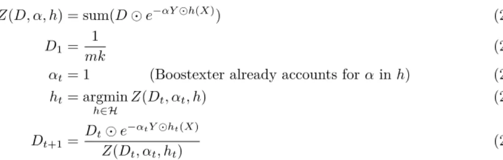
The training algorithm for Adaboost Real.MH is as follows3_{. Let X be a matrix of m examples,}

and Y the associated one-hot encoded matrix for k labels. We define D a distribution over examples and labels. h∈ H are functions (weak learners) that return a confidence matrix over their predictions

for the labels for all examples. At each iteration, the weak learner htwhich minimizes the function Z

is selected. The distribution D is then updated according of the weighted errors of the classifier.

Z(D, α, h) = sum(D⊙ e−αY ⊙h(X)) (2.16)

D1=

1

mk (2.17)

αt= 1 (Boostexter already accounts for α in h) (2.18)

ht= argmin h∈H Z(Dt, αt, h) (2.19) Dt+1= Dt⊙ e−αtY⊙ht(X) Z(Dt, αt, ht) (2.20) where sum(·) returns the sum of all elements of a matrix and ⊙ is the elementwise multiplication. In

Boostexter, αt= 1 and h(X) is defined as follows:

W_bj= sum0(Dt1 [s(X) = j ∧ Y = b]) (2.21) cj= 1 2ln ( W₁j+ ε W₀j+ ε ) (2.22) ht(X) = c1s(X) + c0(1− s(X)) (2.23)

where sum0(·) is the sum over rows of its argument, 1[·] is the indicator function, ε = mk1 , s(.) is a

decision stump which returns 1 if a predicate over X is true, 0 else (typical predicates include presence of a symbolic feature, or the fact that a feature is above a threshold). cj is the confidence of the

decision stump for a given decision according to the weight distribution on the training set.

In the past, Adaboost has been quite popular4_{in the NLP and in particular the NLU communities}

due to its ability to seamlessly account for word n-grams, unknown features, and blend symbolic and continuous features. Gradient boosting (XGBoost) is a variant which is still very popular for its performance especially among Kaggle competition participants.

2.3.2 Deep models

As stated earlier, training a machine learning algorithm consists in finding a set of parameters that minimize a loss L between the predicted label and reference label for all training examples. This minimization process can be achieved through gradient descent techniques which require computation of the gradient with respect to the parameters θ of the loss5 _{for a given training instance. Finding}

analytically the gradient can become diﬀicult depending on the combined loss and inference functions. Yet a neat trick has allowed to automatically compute the gradient of deep function compositions, giving birth to deep learning.

The methods that lie under the deep learning name, are in fact quite a general class of inference functions which can be relied on to compute the loss. In particular, L is expressed as a computational graph of which composing functions need only to be partially derivable in regard of their input. Figure2.1shows a node of the computation graph with two inputs and one output. Using the chain

3_{The one implemented in ICSIBoost (Favre et al.}_2007c_).

4_{Some say that Boostexter is the first classifier you should try when approaching a new problem since it consistently}

yields a strong baseline, as evidenced by the success of related implementations on the MLComp platform (Liang et al.2010).

5_{One very common loss for training classification systems is the cross-entropy loss L}

ce(yt, yp) = ytln yp+(1−yt) ln(1−

(25)

rule, one can compute the derivative of L in regard of each of the parameters of f as the product of the partial derivatives of each component of the computation graph in the paths that link a parameter θi

to L. The back-propagation algorithm consists in using gradient descent to minimize L and propagate the partial derivatives along the graph from L towards the parameters.

f x1 ∂f ∂x1(y) x2 ∂f ∂x2(y) f (x1, x2) y

Figure 2.1: Computational graph node for a function f with two inputs x1 and x2 and one output f (x1, x2). In the forward pass it computes f from its input, while in the backward pass it receives a

desired output and computes the partial derivative of the input for that output.

Functions that can be expressed as computational graphs are somewhat abusively called neural networks6 _{because they often rely on the basic building block of applying a linear transform to the}

input vector followed by an element-wise parameter-free non-linear function such as tanh(W x + b). A number of machine learning approaches can be re-expressed under the deep learning framework, by for instance using a neural network to build a representation from the input, and then feed it to the classifier. Conditional Random Fields can be trained this way (Artieres et al.2010).

Input Representation A typical representation for categorical input such as text is a one-hot vector

(or one-of-n) where all the components are zero except the one which represents the symbolic value of the input. If the input is a vector of features, then a representation can be created by concatenating the one-hot representations for each of the features. Such representations have been widely adopted with shallow models because of the induced sparsity. Since deep models do not rely on this sparsity, they can benefit from richer representations.

The problem with using words as features is that the lexicon is rich and it is very likely to encounter words at test time which are unknown from the training set. This is especially relevant for languages with a productive morphology. In addition, lexicology shows that words have a range of relationships (such as synonymy, hyperonymy, grammatical traits) which are not encoded by one-hot representations. In order to alleviate both problems, a number of techniques under the name “word embeddings” have been proposed. Most of them rely on the distributional hypothesis according to which words occurring in similar contexts tend to have similar meaning (Harris1954).

Pioneered by techniques like LSA (Deerwester et al. 1990), the general idea is to build a low-dimension approximation of a cooccurrence matrix between words in a given window, built on a very large corpus of text. The recent model GloVe builds vector representations for words so that their dot product approximates the log of their cooccurrence (Pennington et al. 2014). The skip-gram model used in word2vec (Mikolov et al.2013) and fasttext (Bojanowski et al. 2016), two other well-known techniques, makes sure the dot-product of words that occur in the same context is higher than that of words which occur in different contexts. Instead of words, one can use subword-units such as mor-phemes (Qiu et al.2014) or supra-units such as subtrees from the dependency parse (Levy et al.2014) in order to represent word meaning, obtaining embeddings with different properties. It has been shown that word embeddings exhibit the interesting behavior that linear transformations in the representa-tion space encode linguistic regularities, such as plural, gender, or semantic relarepresenta-tionship (Mikolov et al.2013). While a number of evaluation corpora have been built to assess that property, it seems to

(26)

be valid only for frequent words, and we are yet to see concrete applications which benefit from it. Recent work on building multilingual word embeddings seeks cross-lingual representations in order to build NLP systems that can be transferred from one well-resourced language to another less-resourced language (Ammar et al.2016b). Word embeddings have flooded NLP conferences, and it is diﬀicult to cite all the work related to their computation, evaluation and use (Li et al.2018).

Once computed, word embeddings can be used to initialize lookup layers in neural networks, which are either fixed so that the embeddings for unknown words7_{can be used at test time, or learned with}

the rest of the model (fine-tuned). Embeddings can be used for other features than words, such as morphology, or even characters.

Convolutional neural networks Convolutional neural networks (CNN) originated in the computer

vision community where they were developed to simulate the detection of small patterns by receptive fields8 _{in the visual cortex (LeCun et al.} ₁₉₉₈_{). In the context of natural language processing, they}

are more reminiscent of the bag-of-word hypothesis because they provide a location invariant. In fact, a typical CNN recognizes word n-grams in a word sequence.

Let x1. . . xn be a sequence of words, a convolutional filter at a position i and with window length

l can be defined as:

convl(x, i) = σ(W vec(xi−l

2:i+

l

2) + b) (2.24)

where σ(·) is an activation function, often ReLU (Nair et al. 2010), vec(·) is an operator which

con-catenates its input vectors in order to make a single vector, W and b are trainable parameters of the layer. The convolutional filter is then repeated for all positions i (sequence boundaries are padded with either special vectors or a continuation of the input). While this filter is known to learn a sequence of l word embeddings, multiple such filters can be used in parallel in order to learn multiple n-grams. This is achieved by increasing the number of columns of W and b.

A pooling operator is then introduced in order to provide position invariance, for instance the max− pooling operator uses the location for which the activation is maximum, therefore acting as a bag of n-grams.

pool_max(x) =maxn

i=1 convl(x, i) (2.25)

While variants have been proposed, CN N (x) = poolmax(x) is one of the most popular

implementa-tions. It can learn which embedding n-grams are important in the input irrespective of their location. Because computations can be parallelized across n-gram location, the eﬀiciency of CNNs makes them specifically suitable for processing large inputs.

Recurrent neural networks Recurrent neural networks (RNN) operate over a sequence of

obser-vations / predictions and maintain a hidden state which is updated after seeing each observation. They can be trained by unrolling them through time, and treating them as a large DNN where some weights are shared across time steps. A simple Elman recurrent neural network might be implemented as:

h0= 0 initial state (2.26)

ht+1= tanh(Wrxt+ Urht+ br) recurrence (2.27)

yt= softmax(Woht+1+ bo) output (2.28)

Where h0is the initial state, xtand htare the input and hidden states at time t, ht+1is computed as

a function of xt and ht and used both for the next time step and the prediction of the label ytin the

output layer.

7_{Words existing in the embedding training corpus, but not in the NLP system trained for the target task.}

8_{CNNs share their weights between receptive fields, obtaining position independence. One may wonder how the visual}

(27)

This kind of architecture is typical of tagging tasks, but recurrent neural networks can be used for other tasks such as classification (sentiment analysis), text generation (caption generation) or transduction (machine translation, summarization, conversational agents). For classification tasks, instead of predicting one label per time step, one can input the hidden state at the end of the sequence to a decision layer which performs classification. This RNN is called an encoder. Similarly, the initial state h0 can be replaced by a representation computed with another neural network in order to

condition the predictions on a factor (such as the image for caption generation). This RNN is called a decoder. The encoded-decoder approach where an input is read, and then an output is generated is widely adopted for machine translation (Sutskever et al.2014).

RNNs are trained by unrolling the network of a number of time steps, and back-propagation is truncated after T time steps to render the problem tractable.

Cells In order to better model long-term dependencies, a number of variants have been proposed for computing the hidden state. LSTM (long short-term memory) cells use a gating mechanism for allowing the model to learn when to memorize a value from the input and when to use it:

it= σ(Wixt+ Uiht+ bi) input (2.29)

ft= σ(Wfxt+ Ufht+ bf) forget (2.30)

ot= σ(Woxt+ Uoht+ bo) output (2.31)

c′_t= tanh(Wcxt+ Ucht+ bc) cell state (2.32)

ct+1= ft⊙ ct+ it⊙ c′t (2.33)

ht+1= ot⊙ tanh(ct+1) (2.34)

LSTM(xt, ht, ct) = (ht+1, ct+1) (2.35)

An interesting aspect of LSTMs is that eq.2.33creates a path where the gradient does not cross any non-linearity, which is supposed to reduce the gradient vanishing problem. Highway layers use the same idea to ensure the propagation of the gradient in multilayer architectures (Srivastava et al. 2015a). A number of variants of LSTMs have been proposed in order to carry fewer parameters, or model different phenomena. Gated Recurrent Units (GRU) are often used in the NLP community because on most problems they are faster than LSTMs without significant performance degradation (Chung et al.2014). zt= σ(Wzxt+ Uzst+ bz) update (2.36) rt= σ(Wrxt+ Urst+ br) forget (2.37) ht= tanh(Whxt+ Uh(rt⊙ st) + bh) input (2.38) st+1= (1− zt)⊙ ht+ zt⊙ st new state (2.39) GRU(st, xt) = st+1 (2.40)

Encoder-decoder architectures A language model can be implemented with RNNs by predicting the next word given the current word and the hidden state which encodes the history without a fixed horizon like n-grams. Such a language model can be conditioned on some arbitrary input in order that it gets biased towards generating different word sequences given different inputs. The bias could introduce additional information concatenated to word representations or as the initial hidden state (instead of setting it to 0). The additional information could be topics (Mikolov et al.2012), a representation for an image (Xu et al. 2015) or some arbitrary data. Such a model is often called a

decoder. Conversely, the hidden state after seeing a number of words is supposed to carry that history

and can be used as a representation of its content. By dropping the RNN output layer and leveraging the hidden state after seeing the last word, one can use it as representation for categorizing the text (for sentiment analysis for example (Rouvier et al.2016a†)). Such an RNN is called encoder.

(28)

The encoder-decoder framework first creates a representation of the input, and then generates a sequence of words conditioned on that input. The greatest success of this idea is Neural Machine Translation (Bahdanau et al.2014) which uses an encoder to create a representation of a sentence in the source language, and then generates the translation in the target language using a decoder. Another interesting application is learning conversational agents and question answering systems which given a representation of a question generate an answer word by word (Vinyals et al.2015). Encoders and decoders need not be RNNs and could be any kind of representation-generating and output-generating neural networks. The point of the approach is that both are trained end-to-end so that the learned representations are tailored to the generation task (text to text, image to text, text to image, etc.).

Advanced architectures A range of architectures have been proposed to extend the speed of

se-quence prediction neural networks over large inputs such as speech data.

Quasi-Recurrent Neural Networks (Bradbury et al. 2016) and variants make sure that a large portion of matrix multiplications involved in computing activations of a sequential layer can be par-allelized. The simplest form consists in only using a forget gate, so that the input transformation zt

can be computed for a whole sequence at once in a single matrix multiplication.

zt= tanh(W xt+ b) (2.41)

ft= σ(W xt) forget gate (2.42)

ht= ft⊙ ht−1+ (1− ft)⊙ zt (2.43)

QRNNs have been shown to perform as well as LSTMs on a few tasks requiring more layers but at a fraction of the execution time.

This idea can be extended to fully convolutional networks with a non-recurrent gating mechanism. Gated Linear Units (Dauphin et al.2016) apply two convolutions on the input, and use the second one as gating mechanism for the first one. Again, this architecture works if multiple layers of GLU are stacked, the convolution window at a given layer helping characterize a larger context.

ht= conv (1) l (x, t)⊙ σ ( conv(2)_l (x, t) ) (2.44) Another interesting approach to accessing long term contextual information is dilated convolu-tions (Yu et al.2015) which operate like convolutions, but on inputs distant of a dilatation factor d. At each layer, the dilatation factor is increased in order to reach further context. This approach was successfully applied to the text-to-speech and speech-to-text tasks (Oord et al.2016).

2.3.3 Additional design patterns

Bidirectional networks The first issue with RNNs is that even though they can potentially

mem-orize long-distance phenomena, they are limited by their temporal causality. A straightforward exten-sion consists in building two RNNs, one that runs from forward in time from 0 to n, and another that runs backwards from n to 0. Their output at each time step is then concatenated to produce a hidden representation which is both influenced by the past and the future.

hf₀= hb_n= 0 (2.45) hf_t= RNNf(hf_t₋₁) (2.46) hb_t = RNNb(hb_t+1) (2.47) ht= hft⊕ h b t (2.48)

where ⊕ is the concatenation operator, ·f _and _·b _{respectively correspond to variables linked to the}

forward and backward RNNs. The produced representation htcan then be used to predict, for instance,

(29)

Multilayer networks In order to build more abstract representations, it is common practice to stack

multiple layers of neural networks which each feeds from the representations created by underlying layers. In the vision community, it has been shown that layers closer to the input recognize simple shapes while deeper layers match more abstract concepts. In NLP, multiple layer CNNs will be able to capture combination of n-grams and multilayer RNNs can leverage phrase-level or sentence-level representations.

Multilayer architectures are riddled with the same gradient vanishing problem that RNNs suffer along the time dimension, but from layer to layer. DenseNets for instance, consist in connecting each layer to all the subsequent layers, including the output, therefore providing a shorter path for supervi-sion propagation (Huang et al.2016). Residual connections (He et al.2015), consist in systematically adding the input of a layer to its output:

Li+1= F (Li) + Li residual connection (2.49)

where Li is the output at layer i and F (·) is the non-linear function performed by a given layer. In

this topology, there is a linear path from each layer to the output for gradients to propagate. The last class of multilayer connection is reminiscent of LSTMs as it includes a gating mechanism which choses between a layer’s input and its transformed output (Srivastava et al.2015b).

gi= σ(W Li+ b) gate (2.50)

Li+1= gi⊙ F (Li) + (1− gi)⊙ Li highway connection (2.51)

where gi is a gate vector,⊙ is the elementwise multiplication. Here, if gi= 1, the layer output is used,

while if gi = 0 its input is used.

Attention Mechanisms One observation with RNNs and in particular encoder-decoder networks

is that they tend to forget about specific events that occurred at the beginning of the sequence they process (Bahdanau et al.2014). The problem is that fixed-sized representations (such as the hidden state of an RNN) cannot account for all the information available in a variable-size input. Loosely modeled after attention in human cognition, the attention mechanism in neural networks creates a global representation given a sequence of states as a weighted sum over these states. The weight distribution is parameterized on the decoder state so that the neural network can learn to focus on different input states when performing predictions.

Let ejbe an encoder state, and dibe a decoder state, one implementation of an attention mechanism

in an encoder-decoder can be defined as

αi= softmaxj(falign(di, ej)) (2.52)

ATTNi=

∑

j

αi,jej (2.53)

where falign is a function which computes an alignment score between a pair of encoder and decoder

states. Two broad types of alignments have been proposed: additive and multiplicative attentions (Bah-danau et al.2014; Luong et al. 2015):

f_align+ (di, ej) =v⊤tanh(W1di+ W2ej) additive attention (2.54)

f_align× (di, ej) =d⊤i W3ej multiplicative attention (2.55)

where v is a parameter vector, W1, W2and W3 are parameter matrices.

In machine translation, attention mechanisms tend to learn an alignment between source and target words, and can be used to map unknown source words to target locations and translate them separately. Attention mechanisms are not limited to RNNs and can be applied to any representation, such as convolutions in images (Xu et al.2015). In particular, they are used to implement memory lookups in memory networks (Sukhbaatar et al.2015), and can even replace RNNs when stacked as multiple layers and combined with a position-encoding representation (Vaswani et al.2017).

(30)

Ensembles Since gradient descent is not guaranteed to find the optimum of a non-linear loss

func-tion, different random initialization can lead to very different models although they have similar per-formance. Creating model ensembles by averaging the pseudo-probability score vectors they generate, has consistently led to large performance increase (Zhou et al.2002a; Gong et al.2017; Józefowicz et al.2016) but reminds us that we are lacking insight on the true capacity of models and that empirical evidence of the superiority of a given model is relative.

Architecture Search One problem with deep learning is that there is no guarantee that a given

architecture is the best for a given problem. Practitioners often rely on empirical search for the best set of hyper-parameters for a system by running many training iterations in parallel and maximizing performance on a development set. This very costly activity is a crucial component of successful systems and a typical setback for beginners. This area of research is very active and has yielded interesting results.

One can train a neural network to generate architectural parameters for another neural network. (Zoph et al.2016) have shown that alternative gating mechanisms for LSTMs could be found by a system trained this way leading to improvements on diﬀicult benchmarks. Other efforts look at ways of improving the eﬀiciency of covering a large search space (Liu et al.2018).

2.4 Evaluation

While the machine learning community has created a large set of loss functions addressing many needs, they all have in common that they are defined with the objective of facilitating the loss minimization problem. For example, losses used in deep learning should be easily decomposed in a computation graph from which a gradient can be derived. However, natural language processing problems have specifics that might not completely match those requirements. In this context, the machine learning loss is used as a proxy for the real metric used for system evaluation. Such metrics are defined by incorporating task specificities (such as the presence of multiple references as in machine translation), and relating them to the end applications (choice of class weight in a classification experiment).

Evaluation in NLP can be devised in two categories. Manual evaluation involves judges who look at each instance labeled by a system and devise a rating for it; Automatic evaluation leverages a hand-annotated corpus in order to streamline the evaluation process. A completely automatic evaluation metric, one that would not require human intervention, is still elusive because there is no sensible theoretical model to drive its definition. If such metric existed, it could be leveraged by machine learning to build better systems.

2.4.1 Manual Evaluation

Manual evaluation is necessary when a ground truth corpus cannot be easily and cheaply built. It is the case for instance in generative tasks such as machine translation or summarization, and highly subjective tasks such as emotion and sentiment classification. Irrespective of the method for manual evaluation, one fundamental issue is that humans are not consistent in their judgment. Due to the vagueness of the evaluation procedure (if it wasn’t vague, it could be easily implemented as a program), judges tend to disagree among them and be inconsistent in time (due to the learning effect, the fact that judges get used to a repeated task). Therefore, it is important to use multiple judges per evaluated item, and to use techniques such as the Latin square design to limit sequential effects (Bradley1958).

Likert Scales Likert scales are dimensions in which an instance can be evaluated according to a continuous value or more commonly discrete values in an interval. For example, the automatic summa-rization community has used two scales for evaluating the quality of a summary: readability/fluency and overall responsiveness. The first one assesses whether the summary is written in well-formed

Contextual language understanding Thoughts on Machine Learning in Natural Language Processing

HAL Id: tel-02470185

https://hal-amu.archives-ouvertes.fr/tel-02470185

Submitted on 7 Feb 2020

HAL is a multi-disciplinary open access

archive for the deposit and dissemination of

sci-entific research documents, whether they are

pub-lished or not. The documents may come from

teaching and research institutions in France or

abroad, or from public or private research centers.

L’archive ouverte pluridisciplinaire HAL, est

destinée au dépôt et à la diffusion de documents

scientifiques de niveau recherche, publiés ou non,

émanant des établissements d’enseignement et de

recherche français ou étrangers, des laboratoires

publics ou privés.

Machine Learning in Natural Language Processing

Benoit Favre

To cite this version:

Benoit Favre. Contextual language understanding Thoughts on Machine Learning in Natural

Lan-guage Processing. Computation and LanLan-guage [cs.CL]. Aix-Marseille Universite, 2019. �tel-02470185�

Thoughts on Machine Learning in Natural Language Processing

Benoit Favre

January 1, 2020

Foreword

Abstract

Contents

I

Contextual Language Understanding

9

II

Summary of activity

79

Part I

Contextual Language

Understanding

Chapter 1

Introduction

Chapter 2

Modern Natural Language

Processing

2.1

An Empirical Approach

2.2 Tasks

2.3 Systems

2.3.1

Standard models

2.3.2

Deep models

2.3.3

Additional design patterns

2.4 Evaluation

2.4.1

Manual Evaluation