Random PDEs: questions of regularity

HAL Id: tel-01468045

https://tel.archives-ouvertes.fr/tel-01468045

Submitted on 15 Feb 2017

HAL is a multi-disciplinary open access

archive for the deposit and dissemination of

sci-entific research documents, whether they are

pub-lished or not. The documents may come from

teaching and research institutions in France or

abroad, or from public or private research centers.

L’archive ouverte pluridisciplinaire HAL, est

destinée au dépôt et à la diffusion de documents

scientifiques de niveau recherche, publiés ou non,

émanant des établissements d’enseignement et de

recherche français ou étrangers, des laboratoires

publics ou privés.

Random PDEs: questions of regularity

Jean-Christophe Mourrat

To cite this version:

Jean-Christophe Mourrat. Random PDEs: questions of regularity. Probability [math.PR]. ENS de

Lyon, 2017. �tel-01468045�

Habilitation à diriger des recherches

Université de Lyon – CNRS

Ecole normale supérieure de Lyon

Unité de mathématiques pures et appliquées

EDP aléatoires :

questions de régularité

Jean-Christophe Mourrat

Document de synthèse présenté le 6 février 2017

JURY

Alice Guionnet

E.N.S. Lyon

Examinatrice

Martin Hairer

University of Warwick

Rapporteur

Grégory Miermont E.N.S. Lyon

Examinateur

Christophe Sabot

Université Lyon 1

Examinateur

Alain-Sol Sznitman E.T.H. Zürich

Rapporteur

Lorenzo Zambotti

Université Paris 6

Examinateur

Remerciements

En premier lieu, je suis très reconnaissant à Martin Hairer, Alain-Sol Sznitman et Ofer Zeitouni d’avoir accepté d’être les rapporteurs de mon habilitation. Merci d’avoir consacré une partie de votre temps précieux à ce travail. Je suis également très reconnaissant à Alice Guionnet, Grégory Miermont, Christophe Sabot et Lorenzo Zambotti d’avoir bien voulu faire partie du jury. Chacun d’entre vous est une source d’inspiration constante pour moi.

J’aimerais dire un immense merci à mes collaborateurs. Ce mémoire donne la plus grande place aux travaux récents réalisés en collaboration avec Scott Armstrong et Tuomo Kuusi d’une part, et Hendrik Weber d’autre part. Difficile de résumer en quelques mots toutes nos aventures ! Je remercie aussi chaleureusement mes collaborateurs lausannois Tom Mountford et Daniel Valesin. A vous tous, je voudrais dire combien j’ai aimé faire ce bout de chemin à vos côtés. Je pense également à mes autres collaborateurs bien sûr, qui m’ont chacun tant apporté.

Et bien sûr, amis et collègues de l’UMPA, merci à vous ! J’apprécie énormément l’ambiance du labo, à la fois mathématiquement stimulante et humainement si bienveillante. Je n’ose pas me lancer dans une liste des gens formidables de l’UMPA et de l’ICJ, ils sont si nombreux.

Merci aux amis non mathématiciens, et qui ne liront jamais ces lignes ! Merci aussi à mes parents pour leur soutien constant. Enfin, merci à Rosanne pour ces années passées ensemble.

Contents

Remerciements iii

Chapter I. Overview 1

1. Homogenization 1

2. Singular stochastic PDEs 16

3. The Anderson model 22

4. The pinning model 25

5. Aging of glassy systems 26

6. The contact process 27

Chapter II. Quantitative homogenization 31

1. Introduction 31

2. Classical regularity theory 32

3. Homogenization and regularity theory 35

4. Subadditive quantities 37

5. Higher-order regularity 40

6. The master quantity J 41

7. Revealing the additive structure 45

Chapter III. The Φ4 _{model 51}

1. Heuristic link between the Ising and Φ4_{models 51}

2. Perspective from quantum field theory 52

3. Convergence of the two-dimensional Ising-Kac model to Φ4 ₅₃

4. Besov spaces and paraproducts 59

5. Global well-posedness of the Φ4 model in the plane 62

6. Global well-posedness of the Φ4 model in three dimensions 64

Bibliography presented for the HDR 69

Bibliography 71

CHAPTER I

Overview

The goal of this document is to survey my research from the completion of my Ph.D. thesis until March 2016. For convenience, the list of the corresponding research articles (including [Mou10, Mou11b, Mou11a] from my Ph.D. thesis) is displayed in a separate section of the bibliography, at the end of this document.

The present chapter aims at giving a bird’s-eye view of my research activity. Besides presenting the results I obtained, I aim to put them in context and underline the links with other developments or questions. Each section presents a different aspect and can be read independently.

Chapters IIandIIIhighlight certain more specific aspects of my research, in relation with Sections 1and2below. Although the presentation is still informal, the mathematics become more precise there.

1. Homogenization

1.1. Qualitative homogenization. Elliptic and parabolic partial differential

equations of second order appear in a large variety of contexts. As an example, consider the diffusion of temperature in a medium. Denote by u(t, x) the thermal energy density at time t and position x. This quantity is proportional to the temperature. In the absence of external sources of energy, we expect the conservation law

∂tu+ ∇ ⋅ j = 0,

where j is the flux of thermal energy. Fourier’s law predicts that this flux is proportional to the gradient of thermal energy: j = −a∇u, which leads to the parabolic equation

(1.1) ∂tu= ∇ ⋅ (a∇u).

Similarly, the steady state thermal energy profile can be recovered by solving the elliptic equation

(1.2) ∇ ⋅ (a∇u) = 0,

with suitable boundary conditions.

The generality of this derivation makes it clear that the equations (1.1) and (1.2) are relevant in a large variety of contexts. Indeed, it only relies on the assumption of Fourier’s law, which can be expected to hold in great generality, at least in the regime of small gradients. Examples include electromagnetism (Ohm’s law), the diffusion of the concentration of a substance (Fick’s law), or the linearization of Lagrange’s equation for minimal surfaces. The diffusion of the concentration of molecules can be understood microscopically as the result of their Brownian movement. In reference to the context of electromagnetism, the matrix a is often called the conductivity.

We are interested in the situation where the medium is heterogeneous. Math-ematically, this translates into the fact that the conductivity matrix a depends on the position within the medium. We assume however that the statistics of the heterogeneities are homogeneous in space. More precisely, we assume that the law

Figure 1.1. The first two drawings display realizations of the “random checkerboard model”, where the conductivity is α Id in the white region, and β Id in the black region. The squares are independently black or white with probability 1/2. In the limit ε → 0, the material becomes equivalent to a homogeneous material of conductivity√αβ Id.

of the mapping Rd_{∋ x ↦ a(x) is invariant under translations by any vector of Z}d_.

We also ask that this law be ergodic under the action of these translations. Finally, we assume that a(x) is symmetric and uniformly elliptic; more precisely, that there exists a constant Λ< ∞ such that for every x,

(1.3) Id≤ a(x) ≤ Λ Id.

We denote by P the law of the coefficient field a, with associated expectation E. We want to consider the situation where the correlation length of the coefficient field is much shorter than the typical length scale at which we want to describe the solution of an equation involving a. In this case, it is reasonable to expect that the local fluctuations of the conductivity will be “averaged out” in the limit of large distances, resulting in an equivalent equation with constant, homogenized coefficients. One way to formulate this assumption of separation of scales is to introduce a small parameter ε> 0, and solve the family of problems

(1.4) {−∇ ⋅ (a (

⋅

ε) ∇uε) = 0 in U,

uε= f on ∂U,

where U is a given domain with Lipschitz boundary, and f is a fixed function with sufficient regularity. The statement of homogenization is that there exists a matrix

a which is constant in space, deterministic, and not depending on f or U , such that

uεconverges to u solution to

{−∇ ⋅ a∇u = 0 in U,_{u= f on ∂U.}

The matrix a is usually called the homogenized or effective matrix. We may say that the solution operator associated with−∇ ⋅ a (_ε⋅) ∇ converges to that of −∇ ⋅ a∇. The result is not specific to the choice of Dirichlet problems.

The fact that we can asymptotically replace the rapidly oscillating coefficient field a(_ε⋅) by a constant one a is illustrated on Figure1.1. This figure is so suggestive that it may lead us to believe that a is simply the average of a. This is however not the case. One way to realize this is to imagine a medium with long and thin vertical rods of very low conductivity, arranged randomly or periodically in the plane. The presence of these rods will have essentially no effect on a flux going in the vertical direction. On the other hand, it will have a dramatic slowdown effect on a flux going in the horizontal direction. This example shows that the computation of a must incorporate geometric information about the random coefficient field; knowing

1. HOMOGENIZATION 3

its one-point statistics is not sufficient. In fact, Figure1.1displays one of the very rare examples where the homogenized matrix is given by a simple formula.

The statement of homogenization was first proved under the assumption that

x→ a(x) is periodic; we refer to [34] for a comprehensive study of homogenization under this assumption. Under the assumptions we stated on the coefficient field

a(x), the result was obtained by Kozlov [147], Yurinski˘ı [200], and Papanicolaou and Varadhan [173].

This result of homogenization can be recast in terms of diffusions in random en-vironment. Indeed, denote by(Xt)t≥0 the diffusion associated with the infinitesimal

generator −∇ ⋅ a∇, with Ea_xits expectation started from x, and let f∈ C_c∞(Rd_{, R).} The function

uε(t, x) ∶= Eaε−1x[f (ε Xε−2t)]

satisfies the equation

(1.5) ⎧⎪⎪⎨⎪⎪

⎩

∂tuε= ∇ ⋅ a (_ε⋅) ∇uε in R+× Rd,

uε(t = 0, ⋅) = f.

As was shown in [173], one can deduce from the statement of elliptic homogenization stated above that this new function uεconverges to u solution to

⎧⎪⎪ ⎨⎪⎪ ⎩

∂tu= ∇ ⋅ a∇u in R+× Rd,

u(t = 0, ⋅) = f.

This can be rephrased in probabilistic terms as (1.6) Ea_ε−1_x[f (ε Xε−2t)] ÐÐ→

ε→0 Ex[f (Bt)] ,

where under Ex, the process B is a Brownian motion starting at x and with

covariance matrix 2a. One can then deduce the convergence in law of εXε−2_⋅ to

B. The precise statement obtained in this way involves an averaging on the initial

starting point of the diffusion, see [173].

A more direct and probabilistic approach to prove the convergence of the rescaled diffusion to Brownian motion was developped by Osada [170]. Putting more emphasis on the process of the environment viewed by the particle and using heat kernel upper bounds, Osada shows that εXε−2⋅converges in law under Pa0 to B,

for P-almost every realization of the coefficient field a. Such a statement is usually called a quenched central limit theorem. The weaker statement of convergence in law under PPa0 is called an annealed central limit theorem.

The approach based on the environment viewed by the particle was extended to general reversible Markov processes by Kipnis and Varadhan [144] (see also [73,74]). This general viewpoint covers at once a random walk evolving on a percolation cluster and a tagged particle in the symmetric exclusion process, among other examples. However, the result takes the form of an annealed central limit theorem.

There are several ways to prove the statement of homogenization. We will fisrt focus on a PDE-oriented approach, in the elliptic setting, with uεsolution to (1.4),

and then outline briefly a more probabilistic approach. A powerful heuristic consists in postulating that the function uε should be well-approximated by a function of

the form

(1.7) uε(x) ≃ u(x) + εv1(x,x_ε) + ε2v2(x,x_ε) + ⋯,

where the functions v1(x, y), v2(x, y), etc. are “reasonable”. This ansatz is called a

two-scale expansion. Under the assumption that the coefficient field is periodic, we would look for v1 such that for each fixed x, the function y↦ u1(x, y) is periodic

(and similarly for v2, etc.). It is indeed natural to expect a form of local limit for

uε− u, in the sense that for each fixed x, the function

y↦ ε−α(uε(x + εy) − u(x))

should have a well-defined limit which would capture the microscopic oscillations of uε, for a suitable choice of exponent α > 0. Formally replacing uε by the

development u(x) + εα_v

1(x,x_ε) in the equation ∇ ⋅ a (_ε⋅) ∇uε= 0 then suggests the

choice of exponent α= 1. The form of the equation also makes it intuitive that the correction v1(x, y) should depend on x only through the quantity ∇u(x). Moreover,

this dependence should be linear. (All this can be checked by doing the explicit replacement of uεby the two-scale expansion ansatz.) In other words, on a scale

intermediate between the microscopic scale ε and the unit scale around point x, the solution uεshould be very close to the solution of a problem homogenizing to an

affine function with slope ∇u(x).

We therefore postpone for a moment the analysis of this two-scale expansion, and study this “affine” solution more precisely. Given p∈ Rd, we wish to find an

a-harmonic function which is as close as possible to the affine function x↦ p ⋅ x. In

other words, we wish to find a function φ(⋅, p) ∶ Rd→ R with slow growth at infinity and such that x↦ p ⋅ x + φ(x, p) is a-harmonic. This last condition can be rewritten as

(1.8) − ∇ ⋅ a(p + ∇φ) = 0.

Here and below, we will often abuse notation and simply write φ instead of φ(⋅, p). In the periodic setting, this equation can be solved with the further requirement that x↦ φ(x) be periodic and of zero mean. In the random setting we chose to work with, we can only ask for∇φ to be a Zd-stationary field with mean zero, in the sense that

(1.9) _{E [∫}

[0,1]d∇φ] = 0.

The function φ is then only well-defined up to a constant, which we may fix by requiring φ(0) = 0. (We will discuss later the possibility of constructing a stationary version of φ, in which case this condition must be lifted.) General arguments then ensure that φ is sublinear, in the sense that

(1.10) r−1(⨏ Br ∣φ∣2₎ 1 2 _a.s. ÐÐÐ→ r→∞ 0,

where Br is the Euclidean ball of radius r centered at the origin, and⨏_Br is the

normalized integral∣Br∣−1∫Br. The function φ is called the corrector (in the direction

of p). Notice that the mapping p↦ φ(⋅, p) is linear.

Equipped with these correctors, we can now come back to the two-scale expansion (1.7) and postulate

(1.11) uε(x) ≃ u(x) + εφ (x_ε,∇u(x)) = u(x) + ε d ∑ i=1 ∂xiu(x) φ (i)₍x ε) ,

where(φ(1), . . . , φ(d)) denote the correctors in the directions of the canonical basis

of Rd_{. This approximation is indeed plausible since it suggests}

∇u(x) ≃ ∇u(x) + ∇φ (x

ε,∇u(x)) ,

in agreement with the idea that the gradient of the solution is close, on a meso-scopic scale, to p+ ∇φ(⋅, p), with a slowly varying p = ∇u(x). The approach to homogenization exposed for instance in [173] consists in defining the difference (1.12) z(x) ∶= uε(x) − u(x) − εφ (x_ε,∇u(x)) ,

1. HOMOGENIZATION 5

and leveraging on the cancellations appearing in the computation of−∇ ⋅ a∇z to infer that z converges to 0 in H1_{(U). The computation reveals that}

(1.13) ap= E [∫

[0,1]da(p + ∇φ(⋅, p))] .

This relation is very natural, since the right side is the average flux of the a-adapted “affine” function with slope p, and the left side is the flux of the affine function with

slope p for the homogenized limit. We also have the energy identity

(1.14) 1

2p⋅ ap = E [∫[0,1]d

1

2(p + ∇φ(⋅, p)) ⋅ a(p + ∇φ(⋅, p))] ,

to which we will return in Subsection1.3. From the convergence of z to 0 in H1_(U),

we can deduce that

∥uε− u∥L2_(U)ÐÐ→

ε→0 0,

as well as the weak convergences in L2(U):

(1.15) ∇uε⇀ ∇u and a∇uε⇀ a∇u.

This weak convergence cannot be improved to a strong convergence, since the convergence to 0 of z in H1(U) can be rephrased as

(1.16) ∥∇uε− ∇u − d ∑ i₌₁ ∂xiu(x) ∇φ (i)₍x ε)∥ L2_(U) ÐÐ→ ε→0 0.

The probabilistic view on homogenization is slightly different, although the correctors also play a central role. In this view, the corrector provides us with harmonic coordinates enabling to turn the diffusion into a martingale. More precisely, the condition that x↦ p ⋅ x + φ(x, p) be a-harmonic can be rephrased as the fact that t↦ p ⋅ Xt+ φ(Xt, p) is a martingale. We thus deduce a decomposition of p ⋅ Xt

as

p⋅ Xt= (p ⋅ Xt+ φ(Xt, p)) − φ(Xt, p),

where the term between parentheses is a martingale, and the remainder φ(Xt, p)

is hopefully of lower order. One can then show that the martingale rescales to a Brownian motion. This consists in checking that the associated quadratic variation grows asymptotically linearly. This can be obtained as a consequence of the ergodicity of the process of the environment seen by the particle. In this way, one obtains a quenched central limit theorem for this martingale part. There remains to show the asymptotic smallness of the remainder φ(Xt, p). At this stage, we only have the

relatively weak information (1.10) on the sublinearity of the corrector. This limits us a priori to an annealed control of this remainder, resulting in an annealed central limit theorem for Xtitself.

The general problem driving my research in the area is to make the statement of homogenization quantitative, in any of the essentially equivalent forms outlined above. This requires to strengthen the mixing assumption on the coefficient field. For simplicity, we will assume that the coefficient field has a finite range of dependence (and sometimes make the stronger assumption that it can be written as a local function of a field of i.i.d. random variables).

Until recently, little was known about this problem. One notable exception is the result of Yurinski˘ı [201] giving a rate of convergence of uε to u in the elliptic

setting, in dimension d≥ 3. The rate of convergence is εα, but the exponent α> 0 is not explicit.

A related question concerns efficient approximations of the homogenized con-ductivity a. The formulas (1.13) or (1.14) are difficult to use for practical purposes, since evaluating the right sides of these identities requires to solve the corrector

equation on the full space, and then compute an expectation involving this corrector. One can replace the expectation on the right side of (1.13) by a space integral

⨏_B

r

a(p + ∇φ(⋅, p)),

which is asymptotically justified in the limit of large r, by the ergodic theorem. We can also replace the corrector itself by a finite-volume approximation (e.g. we approximate the function x↦ p ⋅ x + φ(x) by the solution to the Dirichlet problem on a very large box, with the affine boundary condition x↦ p ⋅ x.) Bourgeat and Piatnitski [45] showed that under suitable mixing assumptions, such approximate schemes yield an error of εα, but again the exponent α> 0 is not explicit.

From the probabilistic perspective, the question is phrased in terms of quantita-tive central limit theorems for the diffusion in random environment. Over the past ten years, an intense research has focused on the related but slightly different ques-tion of obtaining quenched central limit theorems under the most general possible conditions. This research has focused on the discrete counterpart of the diffusion process, which is often called the random walk among random conductances. As was explained above, the difficulty consists in showing that t−12φ(X_t, p) converges

to 0 in Pa

0 probability, for almost every realization of the coefficient field a. One

possibility would be to try to improve on the sublinear growth estimate (1.10). The route chosen instead consists in showing that the law of Xt is sufficiently spread

out that the bound (1.10) is sufficient to conclude. This relies on heat kernel upper estimates. Proofs of these heat kernel bounds for the random walk on supercritical percolation clusters were obtained by Mathieu and Remy [158] and Barlow [21]. The proof of quenched central limit theorem for this walk was obtained by Sidoravicius and Sznitman [185] in dimension d≥ 4, and then in every dimension by Mathieu and Piatnitski [157] and Berger and Biskup [35]. The arguments were then extended in a series of works [41,156,13] to cover arbitrary i.i.d. conductance fields, provided that the set of non-zero conductances defines a supercritical percolation cluster.

1.2. Quantitative homogenization – the nonlinear approach. The

prin-cipal difficulty in quantifying stochastic homogenization is that solutions are nonlin-ear, nonlocal functions of the coefficient field. In other words, there is no simple method to transfer the strong mixing properties we assume on the coefficient field to the solutions themselves.

One approach to overcome this difficulty is to use concentration inequalities that hold for possibly nonlinear functionals. The prototypical example is the Efron-Stein inequality. This inequality states that if X = (X1, . . . , Xn) are independent

random variables, and if (X1′, . . . , Xn′) is an independent copy of X, then for every

function F , (1.17) Var (F (X)) ≤1 2 n ∑ i=1 E [(F (X1, . . . , Xi−1, Xi′, Xi+1, . . . , Xn) − F (X)) 2 ] . One of the early applications of this inequality in the context of quantitative homogenization is due to Kesten [143], who obtained his celebrated variance upper bound for first passage percolation using this inequality.

In my Ph.D. thesis, I got interested in showing quantitative estimates on the rate of convergence to equilibrium of the process of the environment seen by the particle. This question was motivated by the problem of identifying the scaling limit of a toy model for aging, see Section 5. I used the Efron-Stein inequality to implement a Nash-type strategy [149, 37] and obtain a sub-optimal, but explicit polynomial rate of convergence for this process [Mou11b]. From a probabilistic point of view and in the discrete setting, applying the Efron-Stein inequality asks for comparing expectations of functionals for two environments differing only on

1. HOMOGENIZATION 7

a single edge. The main reason for the suboptimality of the estimate I obtained is that from this point of view, there is not much to do to control this difference except to use a crude bound involving the probability that the walk touches the edge where the two environments differ.

Simultaneously and independently, Gloria and Otto [115,116] considered the problem of estimating the sharpness of finite-volume approximations of the right side of (1.14) for the computation of the homogenized matrix. In a more PDE-based approach, they also relied on the Efron-Stein inequality to control the variance of quantities involving the corrector, or a finite-volume approximation thereof. The interesting aspect of the PDE perspective is that one can write an equation for the quantities appearing on the right side of (1.17). Indeed, the term inside the square on the right side of (1.17) is essentially a derivative with respect to the value of the conductance on the edge under consideration, and we can write an equation for derivatives of quantities of interest. We illustrate this idea by doing a formal computation for the derivative of the corrector with respect to the value of a conductance e. Our notation is relatively ambiguous at this point, because it is easier to think of this operation in the discrete setting, although we will keep using continuous-space notation. We differentiate the equation (1.8) for the corrector to get

−∇ ⋅ a∇(∂eφ) = ∇ ⋅ 1e(p + ∇φ).

In the expression above, we write ∂eφ to denote the derivative of φ with respect to

the value of the conductance on edge e. Using the Green representation formula, we obtain ∂eφ(x) = ∑ y G(x, y) (∇ ⋅ 1e(p + ∇φ)) (y) = −∇G(x, e)(p + ∇φ(e)), (1.18)

where G(x, y) is the Green function associated with −∇⋅a∇, and we used a summation by parts in the last step. The heart of the work is then to prove sufficiently good estimates on the Green function itself. The technique is inspired by previous work of Naddaf and Spencer [166], who implemented a comparable strategy under the additional assumption that the conductivity matrix is uniformly sufficiently close to the identity (the regime of “small ellipticity contrast”). This work was in turn influenced by their earlier, fundamental contribution to the understanding of the so-called∇φ interface model [165], to which we will return.

By this method, Gloria and Otto could obtain optimal estimates on the quantities they chose to focus on. This was therefore a major milestone in our understanding of quantitative homogenization. In an updated version of [Mou11b], I could show that the questions I considered of convergence to equilibrium of the environment seen by the particle, and their questions of numerical approximation of the homogenized coefficients, are very closely related. In fact, they are equivalent in small dimension, and otherwise the “parabolic” statement concerning the environment seen by the particle is stronger [Mou11b, Section 9]. The realization of this correspondence led to the development of new methods of numerical approximation of the homogenized coefficients [GM12], which are based on Richardson extrapolations. We could identify precisely the order up to which Richardson extrapolations really improve the rate of convergence. Partially inspired by these observations, Gloria, Neukamm and Otto took up the study of the rate of convergence of the process of the environment viewed by the particle. In [113], they obtained optimal convergence rates for this process, in the sense of polynomial moments. As can be glimpsed from the formula (1.18), a crucial ingredient of the proof rests in proving sufficiently strong estimates

on the gradient of the Green function. The estimates proved there are phrased in terms of spatial averages of high polynomial moments of the gradient.

Estimates on gradients of the Green function were subsequently refined by Marahrens and Otto [153], who showed the following. Recall that we denote by

G(x, y) the elliptic Green function. For every p < ∞, there exists a constant C < ∞

such that for every x, y∈ Zd,

(1.19) _{E[∣∇G(x, y)∣}p]1p ≤ C

∣y − x∣d−1,

(1.20) _{E[∣∇∇G(x, y)∣}p]1p ≤ C

∣y − x∣d,

where in the second line, the quantity∇∇G(x, y) denotes the mixed second derivative of G. In other words, one ∇ acts on the first variable, and the other on the second variable. The estimates match the behavior of the constant-coefficient case, and extend the results of Delmotte and Deuschel [75], who showed (1.19) for p= 2 and (1.20) for p= 1 (these weaker estimates were proved without any mixing assumption on the coefficients; see also [31] for a different perspective on this problem). In the work [153], the Efron-Stein inequality is replaced with a stronger log-Sobolev inequality. Strictly speaking, the estimates (1.19) and (1.20) are only true in the discrete setting, due to the possible local irregularity of the coefficient field (which should be irrelevant to the large-scale question of homogenization). The result was extended to continuous equations in [111], with local averages of the gradients replacing these pointwise bounds.

With such estimates, one can prove optimal bounds on essentially every quantity of interest, with a probabilistic control in the sense of polynomial moments. In particular, one can show that in dimension d≥ 3, the corrector can be constructed as a stationary field, and has bounded polynomial moments. In dimension 2, the corrector grows at most logarithmically, in the sense of polynomial moments. For the elliptic problem

(1.21) − ∇ ⋅ a (_ε⋅) ∇uε= f in Rd,

where f∈ C_c∞(Rd_{, R), we have the estimate}

(1.22) E [∥uε− u∥ p Lq_(Rd₎] 1 p ≤ Cε,

in dimension d ≥ 3, where the function u is the solution of the corresponding homogenized problem. In dimension d= 2, assuming further that f is of zero mean, the estimate (1.22) holds up to the multiplication by log12ε−1_.

The important difference between the problem (1.21) and that displayed in (1.4) is that (1.21) is posed in the full space, while (1.4) is posed in a domain. Solutions of problems such as (1.4) display a degraded rate of convergence within a layer close to the boundary of the domain, and the estimate corresponding to (1.22) breaks down. In the random setting, these boundary layers are not well-understood.

I will now discussion those of my contributions that relate to this work, separating them into three groups.

First, in parallel to these developments, I explored the possibility to use the results and methods of the early papers [115,116] of Gloria and Otto to pursue a probabilistic approach to stochastic homogenization. The approach rests on the development and application of quantitative martingale convergence theorem. I initially focused on deriving annealed quantitative central limit theorems, partly because it is simpler technically, and partly because it gives access to the “systematic error” E[uε(x)] − u(x), while the “statistical error” measured by the variance

1. HOMOGENIZATION 9

After a first partial result [Mou12c], (the cause of the limitation is partly explained in [Mou13]), I showed in [Mou14] that for the solution uε(t, x) to the (discrete

version of the) parabolic problem (1.5), we have, for each fixed t> 0, x ∈ Rd _and

δ> 0, the existence of a constant C < ∞ such that for every ε ∈ (0, 1],

∣E[uε(t, x)] − u(t, x)∣ ≤ Cε1−δ,

for arbitrary δ> 0, in dimension d ≥ 3. In agreement with the discussion surrounding (1.5)-(1.6), this estimate is obtained through a quantitative annealed central limit theorem for the random walk in random conductances. The proof of a similar result, based on the method of two-scale expansion, then appeared in [112]. Together with Yu Gu, we pursued the probabilistic approach further in [GM14] and showed that in dimension d≥ 3, for each fixed t > 0 and x ∈ Rd,

(1.23) uε(t, x) = u(t, x) + ε d ∑ i=1 ∂xiu(t, x) φ (i)₍x ε) + o(ε),

where o(ε) is a quantity satisfying ε−1_{E[∣o(ε)∣] → 0 as ε → 0. Despite the heuristic of} the two-scale expansion, this actually came as a surprise. The two-scale expansion, as quantified in [112], shows that the left side of (1.16) is bounded by Cε, from which we can only infer that

∥uε− u∥_L2_(U)≤ Cε.

A signature of the application of the probabilistic method is that the estimate (1.23) holds pointwise, or in other words, for any fixed pair(t, x). Exploring higher-order two-scale expansions, Yu Gu [119] later uncovered a cancellation which enabled him to prove in the elliptic setting that ∥uε− u − ε ∑di=1∂xiu φ

(i)₍⋅

ε) ∥L2= o(ε).

Second, the following question caught my interest. As was already said, it is computationally expensive to compute the homogenized coefficients of a given random field. However, Anantharaman and Le Bris [9, 10, 11] observed that if the medium is a small random perturbation of a homogeneous medium, then there are much more efficient methods to compute the homogenized matrix. This observation follows a long tradition of perturbative formulas for effective parameters of homogeneous materials perturbed by a small periodic or random structure, which date back to the 19th century and go under the names of Clausius-Mossotti, Lorentz-Lorenz, Maxwell, or Rayleigh formulas. The precise setting usually referred to by physicists is the following. From a homogeneous material of conductivity α Id, add unit-ball inclusions of conductivity β Id, with density p≪ 1, in a stationary manner. Then the effective conductivity of the resulting material is

(1.24) (α + αd(β − α)

β+ α(d − 1)p+ o(p)) Id.

This formula was proved by Rayleigh [192] assuming that the balls are arranged along a periodic lattice.

The formula (1.24) rests on the assumption that the inclusions are spherical. One aspect of the contribution of Anantharaman and Le Bris is to observe that for more general inclusions, although no closed analytic formula is expected to exist, we can think of efficient numerical strategies allowing to compute the homogenized matrix. The idea is to write a finite-volume periodic approximation of the homogenized matrix, and formally interchange the limits of large volume and small density of inclusions. By doing so, we obtain the first-order correction by computing a corrector-type quantity in a periodic box containing exactly one inclusion. This computation can be performed efficiently, and should indicate the first-order perturbation to the homogenized coefficients.

The Clausius-Mossotti formula was first proved by Almog [7] in dimension

d= 3, by methods specific to this dimension. In [Mou15a], I justified and extended the picture proposed by Anantharaman and Le Bris, in every dimension and in a discrete setting. The adaptation of the arguments to the continuous setting yields a proof of the Clausius-Mossotti formula in every dimension as a particular case. The result was later generalized to cover general ergodic random fields and expansions of arbitrarily high order by Duerinckx and Gloria [83].

My interest in this problem was also motivated by the question of the behavior of the effective diffusivity of near-critical percolation. More precisely, denote by

a(p) = a(p) Id the homogenized matrix associated with the two-dimensional square

bond percolation (say) of parameter p. As is well-known, the critical percolation pc

is equal to 1/2 in this case. Does there exist an exponent σ such that a(p) ≃ (p−pc)σ

as p→ p+_c? Can we compute σ? Denote by a(n, pc) a finite-volume approximation of

a(pc) = 0 in a box of size n (for instance, a(n, pc) is the expectation of the effective

conductivity between two faces of the box of size n). Does there exist an exponent τ such that a(n, pc) ≃ n−τ? Can the exponents σ and τ be computed? Can we relate

σ and τ through the correlation length, in the spirit of the Kesten relations [142]? Understanding the problem posed by Anantharaman and Le Bris seemed to be a modest but necessary first step towards a better understanding of these problems. However, despite the immense success of the recent work on two-dimensional critical percolation and its critical exponents, it is not at all clear that the exponents σ and τ have a simple expression (although bounds on τ are known, see [141,71]). Physicists have not come up with such a prediction, despite intensive numerical simulation (see [135] for a review). As an illustration of this possibility, the monochromatic two-arm exponent is not known to have a simple expression. In ongoing work with Christophe Garban, we show that this exponent can be expressed as the principal eigenvalue of a (rather singular) differential operator (see http://goo.gl/n0hnqffor a presentation of our contribution).

The third and final set of problems I wish to discuss here is the following. In a sense, the statement of homogenization is similar to a law of large numbers. (This sentence may be confusing, since we saw that homogenization corresponds to a central limit theorem for the diffusion in random environment. Nevertheless, it is fair to say that from a PDE perspective, the statement is a form of law of large numbers. Moreover, even from the probabilistic perspective, the proof of the central limit theorem is ultimately reduced to an application of the ergodic theorem for the environment viewed by the particle; this may be taken as an indication that we are indeed proving a form of law of large numbers after all.) Once sharp estimates are available for the rate of convergence in this law of large numbers, a natural question is to ask if we can actually identify the next-order correction to homogenization. In other words, we look for a CLT-type result for homogenization.

Before proceeding to describe what can be proved in this direction, I wish to explain why such results can be interesting from a practical perspective. To begin with, homogenization per se is appealing because it enables to replace a computationally very expensive problem with rapidly oscillating coefficients by a much simpler, homogeneous problem, described by a few effective parameters. In a sense we will make precise shortly, the same is true of the next-order, fluctuating correction. This fluctuating field is a Gaussian field whose covariance can be described by a new (finite) set of effective parameters, which we may call the

effective fluctuation tensor.

In this spirit, practitioners have long been interested in the problem of recovering the statistics of the original random field from the observation of the large-scale fluctuations of solutions. However, this problem is ill-defined. The new point of

1. HOMOGENIZATION 11

view outlined above suggests instead to focus on trying to determine this effective fluctuation tensor. This can be done by observing the large-scale fluctuation field of any homogenization problem. Once this effective fluctuation tensor is determined, we gain a powerful approximation of the law of the solution to any other homogenization problem.

In line with the qualitative theory outlined in Subsection1.1, it is reasonable to focus first on understanding the large-scale behavior of the corrector. We already pointed out the connection between stochastic homogenization and the so-called ∇φ interface model of statistical mechanics in relation with the work of Naddaf and Spencer [165, 166] (see also the introduction to [GM16b]). In [165], Naddaf and Spencer identified the scaling limit of this model to be a Gaussian free field. It is therefore natural to conjecture that the same should be true of the corrector (see [35, Conjecture 5]). This is however not correct, although the idea suggests the correct scaling exponent. We will give more precise heuristics and description of the result in Subsection1.3below.

An important idea of Naddaf and Spencer is to make use of a representation of correlations due to Helffer and Sjöstrand [134, 186]. This representation is a refinement of the Efron-Stein inequality. It is easiest to describe the inequality in the case of a given family X = (X1, . . . , XN) of independent standard Gaussian

random variables. In this context, a variant of the Efron-Stein inequality states that for every F = F (X), Var (F ) ≤ n ∑ i=1 E [(∂xiF) 2 ] .

The Helffer-Sjöstrand representation of correlation refines this variance estimate into (1.25) _{Var (F (X)) =} n ∑ i=1 E [(∂xiF)(L + 1) −1_(∂ xiF)] ,

whereL is the Laplacian-type operator on the product space L = ∂∗∂=

n

∑

i=1

(−∂xi+ Xi)∂xi.

(The “divergence” ∂∗ is the adjoint to the “gradient” ∂= (∂xi)i with respect to the

Gaussian measure, hence the additional term Xi above.) Since the formula (1.25) is

an identity, it can be polarized into an identity for correlations. In the context of the homogenization of discrete equations, let us assume for simplicity that the random conductances are (nice) functions of standard Gaussian random variables. This is not really necessary for the statement of the Helffer-Sjöstrand representation, but simplifies the application of the chain rule (see [MO14, Remark 2.3]). Under this assumption and in dimension d≥ 3, Felix Otto and I [MO14] used this representation of correlations, together with techniques as exposed above, to obtain a description of the asymptotic behavior of the correlations of the corrector E [φ(0) φ(x)]. Com-pleting the description of the scaling limit of the corrector, Jim Nolen and I proved the asymptotically Gaussian behavior of spatial averages of the corrector in [MN15].

Together with Yu Gu [GM15], we then described the fluctuations of solutions to (1.21). Surprisingly, we showed under similar assumptions that the naive two-scale expansion of uε in terms of the correctors does not suggest the correct scaling limit

for these fluctuations. We also postpone a more precise description of the results obtained there to the next subsection.

1.3. Quantitative homogenization – the additive approach. More re-cently, I took part in the construction of a new approach to quantitative homoge-nization [14], [AM16,AKM15,AKM16a,AKM16b]. As was said in the beginning

of Subsection1.2, in order to make stochastic homogenization quantitative, we need to transfer the assumed mixing properties of the coefficient field into information on the solutions themselves. This is difficult a priori because solutions are nonlinear, nonlocal functions of the coefficients.

The core idea of the new approach we developed is that energy quantities are in fact local, additive functions of the coefficient field. We should therefore focus on studying these quantities first, and derive properties of solutions as consequences.

This new approach is interesting for a number of reasons. First, it allows to widen the range of coefficient fields covered by the theory. Indeed, the “nonlinear” approach outlined in the previous subsection, based on the Efron-Stein inequality or its variants, essentially requires that we assume the coefficient field to be a function of a family of independent random variables. This can be weakened in several ways, but as an example, the nonlinear approach cannot be applied to a coefficient field which is only assumed to be of finite range of dependence. Recall that a random field a is said to be of unit range of dependence if

(1.26) U, V ⊆ Rd, dist(U, V ) ≥ 1

Ô⇒ (a(x))x_∈U and(a(x))x_∈V are independent.

Moreover, the new approach allows to strengthen the stochastic control of the random variables of interest (we are able to show that the fluctuations have Gaussian tails). In my view, the most important point however is to uncover the additive structure of stochastic homogenization. By exposing this additive structure, we ultimately reduce the problem to a question involving sums of random variables satisfying the same mixing properties as the underlying coefficient field, up to an error we can neglect. Stronger results naturally follow from the uncovering of this simple structure.

The fact that homogenization can be related to the convergence of energy quantities was first exposed by Dal Maso and Modica [69,70] (building on previous work of Marcellini [154] in the periodic setting). For a bounded domain U ⊆ Rd

(with Lipschitz boundary) and a vector p∈ Rd_{, denote}

(1.27) ν(U, p) ∶= inf

v∈H1

0(U)

⨏_U 1₂(p + ∇v) ⋅ a(p + ∇v), where H1

0(U) denotes the closure in H1(U) of the set of smooth functions with

compact support in U . One can check that there exists a unique minimizer for this variational problem, which we denote it by v(⋅, U, p) (see e.g. [89, Subsection III.8.2]). The Euler-Lagrange equation associated with this variational problem reads (1.28) ∀ψ ∈ H01(U), ∇ψ ⋅ a(p + ∇v(⋅, U, p)) = 0.

This is the weak formulation of the equation (1.8), with null Dirichlet bound-ary condition on ∂U . In other words, the minimizer v(⋅, U, p) is a finite-volume approximation of the corrector φ(⋅, p).

The quantity ν(⋅, p) is subadditive, in the sense that if U1, . . . , Uk ⊆ U are

pairwise disjoint domains such that∣U ∖ ⋃iUi∣ = 0 (here ∣ ⋅ ∣ denotes the Lebesgue

measure), then (1.29) ν(U, p) ≤ k ∑ i=1 ∣Ui∣ ∣U∣ν(Ui, p).

Indeed, this holds since we can glue the Uiminimizers together and create a candidate

minimizer for ν(U, p). Denoting by

(1.30)

◻

1. HOMOGENIZATION 13

it follows from the subadditive ergodic theorem that ν(

◻

surely and in L1 _{to a deterministic constant as r tends to infinity. Moreover,}

it is straightforward to check from the characterization (1.28) that the mapping

p↦ v(⋅, U, p) is linear, and therefore p ↦ ν(U, p) is a quadratic form. This property

is preserved by passing to the limit. We deduce that there exists a constant matrix

a such that for every p∈ Rd,

(1.31) ν(

◻

Our choice of notation implies that the matrix thus defined is the homogenized matrix. Intuitively, this can be understood from the fact that 1₂p⋅ ap is the result of the

minimization of the functional with constant coefficient v↦ ⨏_U 1₂(p + ∇v) ⋅ a(p + ∇v) in H₀1(U), which selects a-harmonic functions as minimizers. It roughly matches with the relation (1.14). In a loose sense, Dal Maso and Modica [69,70] proved that indeed, the convergence (1.31) implies the statement of homogenization as presented in Subsection1.1(their precise result is phrased in terms of the Γ-convergence of the energy functionals).

This result already offers a glimpse of the additive structure we wish to uncover. Indeed, the quantity ν(⋅, p) is subadditive, and by definition, it is also a local function of the coefficients. Moreover, the result of Dal Maso and Modica strongly suggests to look for a quantification of the statement of homogenization via a quantification of the convergence in (1.31). Roughly speaking, our main task is therefore to show that ν(⋅, p) becomes asymptotically additive. If this can be done, then we expect the next order correction to (1.31) to be governed by a central limit theorem.

This idea is however too naive, because the minimizer of ν(

◻

layer, which implies a next-order correction to (1.31) driven by the behavior of the minimizer close to the boundary. This boundary behavior is irrelevant to the properties of solutions we wish to study. In the remainder of this section, we will ignore this problem and make the false assumption that indeed, the next-order correction to (1.31) is governed by a central limit theorem. We will use this simplifying assumption to describe and explain the structure of the scaling limits of the corrector and the fluctuations of general solutions. We will then return to the problem in Chapter II, explain what can be proved about the quantity ν(⋅, p), and how to overcome the difficulty caused by boundary layers.

Before we proceed to give heuristics for the scaling limits of the corrector and the fluctuations of solutions, we introduce the object that will arise as a scaling limit1. We say that W = (W1, . . . , Wd) is a vector white noise with covariance

matrix Q if for every f = (f1, . . . , fd) ∈ Cc∞(Rd; Rd), the random variable

W(f) ∶= W1(f1) + ⋯ + Wd(fd)

is a centered Gaussian with variance_∫

Rdf⋅ Qf. The set of admissible test functions

can be extended to f ∈ L2_(Rd

; Rd_{) by density. We say that W = [W}

ij]1≤i,j≤d is

a matrix white noise if the vector of its entries is a vector white noise. Given a vector white noise W and a positive-definite symmetric matrix a, we define the

gradient Gaussian free field, or gradient GFF for short, as the random d-dimensional

distribution∇Ψ solving the equation

(1.32) − ∇ ⋅ a∇Ψ = ∇ ⋅ W.

In other words, ∇Ψ is the potential part in the Helmholtz-Hodge decomposition

W = −a∇Ψ + g, where g is the solenoidal (divergence-free) part. We can interpret

1. The remainder of this section essentially follows a presentation given in Banff in July 2015 which can be watched athttp://goo.gl/5bgfpR.

this definition by duality: for every F ∈ C_c∞(Rd

; Rd_{), we set}

(∇Ψ)(F ) = W (∇(−∇ ⋅ a∇)−1_{(∇ ⋅ F )) .}

The function ∇(−∇ ⋅ a∇)−1(∇ ⋅ F ) is the potential part in the Helmholtz-Hodge decomposition of F , and it belongs to L2_(Rd

; Rd_).

This definition is perhaps easier to grasp in dimension d ≥ 3, where we can define the field Ψ itself in a canonical manner. Indeed, in this case, we can interpret (1.32) as defining the centered, stationary Gaussian field with two-point correlation function

E[Ψ(0) Ψ(x)] =∫

Rd∇G(0, y) ⋅ Q∇G(y, x) dy,

whereG(⋅, ⋅) is the Green function associated with the homogeneous operator −∇⋅a∇. If the matrices Q and a are proportional, then an integration by parts reveals that the right side above is a multiple of G(0, x). In this case, we therefore recover the more standard definition of the GFF as the centered Gaussian field whose covariance is given by a Green function. When a and Q are not proportional, the field Ψ is a variant of the more standard GFF with the same scale invariance, but which does not satisfy the spatial Markov property (this was shown in [GM16b], together with the fact that this more general situation does indeed arise in the setting of stochastic homogenization).

Now that our notion of GFF is in place, we can resume our study of stochastic homogenization. As announced, we assume that the quantity ν has been suitably modified (in a way we do not describe here) so that it indeed becomes additive, and the next-order correction to (1.31) is ruled by the central limit theorem. We wish to encode this information in a way that is consistent with changes of the vector p, of the scale r, and of spatial translations. We do so by postulating that

(1.33) ν(x +

◻

1

2p⋅ (a + Wr(x))p,

where W is a matrix white noise, and Wrdenotes its spatial average on scale r:

(1.34) Wr(x) ∶= ⨏

x+◻r W.

(In this heuristic argument, we could also think of Wr as the convolution of W with

a rescaled bump function: Wr∶= W ⋆ χ(r), with χ∈ Cc∞(Rd, R+) such that ∫ χ = 1

and χ(r) ∶= r−dχ(⋅/r).) This encodes in particular the fact that ν(x +

◻

ν(y+

◻

◻

◻

properties of white noise, each coordinate of Wr(x) is of order ∣

◻

d 2 ≪ 1.

We understand that the error in (1.33) is much smaller than r−d2.

Recall that the matrix a is meant to describe the correspondence between gradients of solutions and their associated fluxes. We interpret (1.33) as displaying the correspondence between spatial averages of gradients and fluxes of solutions. More precisely, we interpret (1.33) as meaning that if a function locally minimizes the energy over x+

◻

◻

approximately (a + Wr(x))p.

We now fix p∈ Rd, denote by φ= φ(⋅, p) the corrector in the direction p, and by φr its spatial average on scale r:

φr(x) ∶= ⨏ x+◻r

φ.

The preceding discussion suggests that x↦ p ⋅ x + φr(x) is approximately (a + Wr

)-harmonic. In other words, we expect that the equation −∇ ⋅ (a + Wr)(p + ∇φr) = 0

1. HOMOGENIZATION 15

Figure 1.2. Graphs of the correctors φe1 and φe2 on the top and

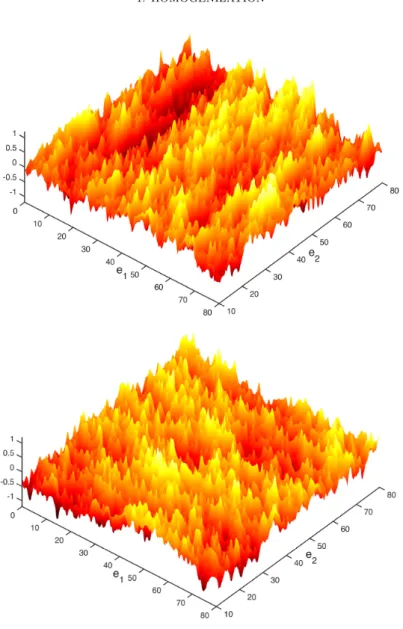
bottom, respectively, for a random checkerboard model in d = 2 (with the same realization). The random matrix is diagonal with independent entries equidistributed between 1 and 10. Notice that the mountain ranges for φeseem to line up in the orthogonal direction to e. The image

is courtesy of Antti Hannukainen (Aalto University).

holds approximately. Rearranging, we obtain

−∇ ⋅ (a + Wr)∇φr= ∇ ⋅ (Wrp).

Since Wr≪ 1, we have ∇φr≪ 1. Therefore, the term Wr on the left side can be

neglected, and we obtain

(1.35) − ∇ ⋅ a∇φr= ∇ ⋅ (Wrp),

up to errors that become negligible in the limit r→ ∞. Equation (1.35) characterizes a gradient GFF, compare with (1.32). Therefore, our heuristic argument suggests

that for a suitably weak topology,

(1.36) rd2(∇φ)(r ⋅)

(law)

ÐÐÐ→

r→∞ ∇Ψ,

where ∇Ψ is a gradient GFF. This result was first proved using the nonlinear approach in [MO14, MN15]. The proof requires somewhat restrictive conditions, and as explained above, a core aspect of this approach is to use the Helffer-Sjöstrand representation of correlations and “follow the computations”. With Armstrong and Kuusi, we gave a proof of this convergence [AKM16a, AKM16b] which is much closer in spirit to the heuristics we just presented, and holds under a finite range of dependence assumption. Figure1.2illustrates the fluctuations captured by this convergence.

Similar heuristics can be devised for solutions to

(1.37) − ∇ ⋅ a∇u = f _{in R}d,

where f∈ C_c∞(Rd) varies on scale ε−1≫ 1. (The function f should be of order ε2in order for u to be of order 1.) We consider the spatial average ur of u over scale r,

1≪ r ≪ ε−1. By the same reasoning as above, we expect urto satisfy the coarsened

equation

−∇ ⋅ (a + Wr)∇ur= f.

We write ur= u + ̃ur, where u solves

−∇ ⋅ a∇u = f, so that

−∇ ⋅ (a + Wr)∇̃ur= ∇ ⋅ (Wr∇u).

As before, we expect the term Wr on the left side to be negligible, so we obtain

(1.38) − ∇ ⋅ a∇̃ur= ∇ ⋅ (Wr∇u).

This approximate identity in law of large-scale spatial averages of solutions to (1.37) was proved in [GM15] using the nonlinear approach, with the important difference that ̃ur is replaced by the spatial average of u− E[u] (instead of u − u). A proof

based on the additive approach has not yet been developed for this problem. As was already pointed out, if we use the formal two-scale expansion u≃ u + ∑iφ(i)∂iu

and the large-scale description of the corrector in (1.35), we are led to a different and incorrect result.

2. Singular stochastic PDEs

In a broad sense, the elliptic PDEs with random coefficients considered in the previous section are “stochastic PDEs”. As is somewhat customary, we will however restrict the use of this name to equations where the randomness appears only as a “thermal” noise, or more precisely, where the part of the equation with derivatives of highest degree is deterministic. In this section, we focus on a particular class of stochastic PDEs, which we may call singular. These PDEs contain a non-linearity, and typically a white noise forcing term. They are such that one does not expect the solution to be a proper function, but only to make sense as a distribution, due to the roughness of the noise. This makes the interpretation of the non-linearity problematic.

We will focus our discussion on two such equations: the Kardar-Parisi-Zhang (KPZ) equation

(2.1) ∂th= ∆h + ∣∇h∣2+ ξ,

and the Φ4 model

2. SINGULAR STOCHASTIC PDES 17

where in both cases, ξ is a space-time white noise.

The KPZ equation has played a central role in the development of the theory. It was introduced in [140] as a model for the growth of an interface subject to fluctuations. In this case, the equation is posed on R+× R, or a subset thereof. We

may postulate that on a mesoscopic scale, the growth of the interface is governed by an equation of the form

(2.3) ∂th= ∆h + F (∇h) + ξ○,

where the Laplacian ∆ encodes a smoothing mechanism, the function F describes the growth mechanism per se, and ξ○is a smooth noise in space and time with short-ranged correlations. The growth mechanism is assumed to be smooth, symmetric:

F(z) = F (−z), and up to a change of time frame, we may assume that F (0) = 0 by

replacing F by F− F (0) if necessary. For some large parameter λ ≫ 1, we consider the change of scale

ˆ h(t, x) ∶= λ−12h(λ2t, λx), ˆξ∶= λ 3 2ξ○(λ2t, λx), so that ∂tˆh= ∆ˆh + λ 3 2F(λ− 1 2∇ˆh) + ˆξ,

and ˆξ converges to a space-time white noise as λ→ ∞. Since F (z) ≃ a2z2for small z,

we see that the non-linear part becomes more and more dominant as we increase the scale. This suggests to “dampen” the non-linearity by replacing F with λ−12F .

Using the asymptotics F(z) ≃ a2z2+ a4z4+ ⋯, we are led to

(2.4) ∂tˆh= ∆ˆh + a2∣∇ˆh∣2+ λ−1a4∣∇ˆh∣4+ ⋯ + ˆξ.

So we may expect that the higher-order terms λ−1a4∣∇h∣4+ ⋯ become negligible in

the limit of large λ. This very informal computation in the spirit of [140] therefore suggests a certain universality of the equation (2.1) as a description of the large-scale fluctuations of growing interfaces. Note that in the derivation of the equation, we were forced to modify the non-linearity along the way in order to weaken it.

While these heuristics are very appealing, making sense of them mathematically is very challenging. Indeed, the solution to the linearized version of the equation (2.1), which reads

(2.5) ∂thlin= ∆hlin+ ξ,

is such that for each fixed t, the function x↦ hlin(t, x) has the regularity of Brownian

motion: it is α-Hölder continuous for every α< 1/2, and no more. In particular, the derivative of hlin is a very singular object, and the square of such an object has no

canonical meaning. In view of this, the Taylor expansion performed in (2.4) looks very worrisome, and indeed it is misleading, although the non-linearity does become quadratic in the limit — more on this below.

A naive attempt at defining a solution to (2.1) consists in regularizing the noise, e.g. by convolving the white noise field against a smooth bump function of scale ε to get a smooth noise ξε, then solve

∂thε= ∆hε+ ∣∇hε∣2+ ξε,

and try to pass to the limit ε→ 0. However, the term ∇hεbecomes more and more

singular as ε tends to zero, and the sequence hεdiverges. In short, we have to accept

the fact that we cannot give a classical meaning to (2.1) as stated. We need to take a step back and find a suitable modification of (2.1) that enables to make sense of the equation, but that is sufficiently minor to ensure that the solution we find is physically relevant to interface growth models. Bertini and Giacomin [36] made

a major step in this direction. First, by a formal Cole-Hopf change of unknown function Z∶= exp(h), one arrives at

(2.6) ∂tZ= ∆Z + Zξ.

This is a linear equation in Z. One can make sense of this equation by writing its mild formulation and interpreting the integral involving Zξ as an Itô integral (thus avoiding to define the product Zξ per se). Moreover, Z is strictly positive almost surely [164], so we can decide to define the solution to (2.1) as h∶= log(Z). This may seem somewhat ad hoc, but strikingly, Bertini and Giacomin showed that the process thus defined indeed arises as the scaling limit of a certain model of interface growth. This model can be mapped to a particle system on the line, via the identification between the presence/absence of a particle and the slope of the interface being±1. The dynamics of the particle system is that of simple exclusion, with an asymmetry that is slowly tuned down to zero, in the spirit of the gradual taming of the nonlinearity performed in the heuristic argument leading to (2.4).

If one regularizes the noise in space in (2.6) and writes

∂tZε= ∆Zε+ Zεξε,

an application of Itô’s formula reveals that the function hε∶= log(Zε) actually solves

the modified equation

(2.7) ∂thε= ∆hε+ ∣∇hε∣2− Cε+ ξε,

where Cε∼ c/ε as ε tends to 0, for some constant c > 0. By the intermission of the

Cole-Hopf transform, we therefore conclude that

(1) for a suitable choice of Cε ∼ c/ε, the solution hε to (2.7) converges to a

non-trivial limit h;

(2) this limit h can be obtained as the scaling limit of a natural model of interface growth.

Physicists would say that we added a counter-term Cε to balance the divergence

of the term ∣∇hε∣2. We may also say that we have “renormalized” our original

equation (2.1). The introduction of this additional constant Cεamounts to a shift

in time of the solution, and is therefore very benign from a physical point of view: it simply indicates that the naive guess about the asymptotic speed of growth of the interface has to be corrected by a diverging constant.

While this development was of course a major progress in the mathematical understanding of the KPZ equation, a core aspect of the approach lies in the avail-ability of the Cole-Hopf transformation, which in effect linearizes the equation. A downside is that it completely avoids trying to make sense of the equation (2.1) directly. Moreover, the passage from discrete to continuum also requires a micro-scopic version of the Cole-Hopf transform (first observed in [98]), and therefore the set of interface growth models for which the approach of [36] applies is rather rigid (see however [77,65]).

As far as the continuous equation is concerned, these shortcomings were overcome by Hairer, first for the KPZ equation per se [125], and then within a much more general framework covering at once the two equations (2.1) and (2.2) of interest to us here [126]. The key property that the equation needs to satisfy is that of

subcriticality, or in the language of quantum field theory, the equation must be superrenormalizable.

Loosely speaking, a (formal) stochastic PDE is said to be subcritical if the non-linearity is dampened when we zoom in on a (formal) solution. For the KPZ equation in one space dimension, we have already observed that the non-linear term formally blows up when we consider the rescaled solution on larger and larger scales.

2. SINGULAR STOCHASTIC PDES 19

Reversing the scaling by letting λ tend to zero instead of infinity corresponds to zooming on the fine details of the solution; this has the opposite effect of reducing the strength of the non-linearity. This equation is therefore subcritical.

We now perform the same analysis for the Φ4 model (2.2), allowing the space dimension d to be arbitrary. (Background and motivation for this equation will be provided in Chapter III.) The change of scale

ˆ

X(t, x) ∶= λd−22 X(λ2t, λx), ˆξ(t, x) ∶= λ d+2

2 ξ(λ2t, λx)

is so that ˆξ and ξ have the same law, and moreover,

(2.8) ∂tXˆ = ∆ ˆX− λ4−dXˆ3+ λ2a ˆX+ ˆξ.

The non-linearity is tamed down as we let λ tend to zero if d< 4: the equation is therefore subcritical in these cases.

In spatial dimension d= 1, the solution is expected to be a proper function (as explained above in the context of the KPZ equation), and therefore the stochastic PDE can be made sense of by classical methods. The dimensions of interest to us are thefore d∈ {2, 3}.

When the equation is subcritical, we can hope to obtain an existence theory for the equation by developing a generalized form of “Taylor expansion” of the solution, where the first order of the expansion is described in terms of the solution to the linear equation

(2.9) ∂tZ= ∆Z + ξ.

In spatial dimension d= 2, this idea is by now well-understood since the work of Da Prato and Debussche [68] (earlier contributions using different approaches include [138, 3, 177, 161]). The argument proceeds in two steps. First, one can define “renormalized” (or Wick) powers of the solution Z to the linear equation: writing

Zεfor the solution to (2.9) with ξ replaced by the smoothed noise ξε, there exists a

constant Cε which diverges logarithmically as ε→ 0 and such that

(2.10) Zε2− CεÐÐ→ ε→0 Z ∶2∶_{, Z}3 ε− 3CεZÐÐ→ ε→0 Z ∶3∶_,

and so on with higher order Hermite polynomials. Second, the property of subcriti-cality suggests that the difference Y ∶= X − Z should have better regularity than

X itself, or in other words that we should look for a “Taylor expansion” of X of

the form X = Y + Z, where Z is hopefully sufficiently regular to enable to write a meaningful equation for it. Indeed, formally starting from (2.2) gives

(∂t− ∆)Y = −(Y + Z)3+ a(Y + Z).

Expanding the cubic power leads to undefined terms, but the construction of the renormalized powers of Z suggests the renormalization rules

Z2↝ Z∶2∶, Z3↝ Z∶3∶,

so that the equation above becomes

(2.11) (∂t− ∆)Y = −Y3− 3Y2Z− 3Y Z∶2∶− Z∶3∶+ a(Y + Z).

As will be explained in more details in ChapterIII, in spatial dimension d= 2, the renormalized powers of Z belong to every function space of negative regularity, and therefore the equation (2.11) can be solved with Y being almost twice differentiable. This defines a notion of solution to (2.2), and moreover, the solution depends continuously on the triple(Z, Z∶2∶, Z∶3∶) (for a suitable topology). If we replace the