Adaptive Output Feedback Control of Aircraft
Flexible Modes
Sangeeth saagar Ponnusamy, Joël Bordeneuvue Guibé
ISAE, Université de Toulouse, 10 Avenue Edouard BelinToulouse, France
[email protected], [email protected]
Abstract— The application of adaptive output feedback
augmentative control to the flexible aircraft problem is presented. Experimental validation of control scheme was carried out using a three disk torsional pendulum. In the reference model adaptive control scheme, the rigid aircraft reference model and neural network adaptation is used to control structural flexible modes and compensate for the effects unmodeled dynamics and parametric variations of a classical high order large passenger aircraft. The attenuation of specific low and high frequency flexible mode depending on linear controller design specifications and adaptation parameters were observed. The effectiveness of the approach was seen in flexibility control of the high dimensional, nonminimum phase, nonlinear aircraft model with parametric uncertainties of wind and unmodeled dynamics of actuators and sensors.
Keywords- Adaptive control, Flexible structures, Neural network, Flexible Aircraft.
I. INTRODUCTION
Aircraft control is a highly complex problem to obtain the optimum compromise between safety, stability, manoeuvrability and comfort. Classical frequency separation assumptions used to segregate the structural rigid and flexible modes in designing the control system no longer holds true nowadays due to multiple reasons ranging from the use of lighter materials to fuel transfer in new generation aircrafts. The limitation of conventional control methods in turn demands newer active control strategies. Adaptive output feedback augmented control for flexible systems has been studied by Bong Jun-Yang et al [3] and validated on real time systems [1]. Neural network adaptive control was applied to flexible aircraft pitch control by Nakwan Kim et al [4]. Laurent Bako et al [2] showed the validity of the scheme to the control objective of reducing oscillations due to flexibility in aircraft wings. The present study is an extension of the neural adaptive control methodology developed in [1] & [2] to control flexible modes of high order aircraft with 193 states using a reduced order rigid reference model of order 2. The paper is organized as follows, in section II the formulation of the control scheme is given, followed by the experimental validation similar to [1] in section III. The control scheme is applied to the flexible aircraft problem in section IV, where the control objective of reducing structural oscillations was studied for two different cases of linear controllers. Conclusions are given in section V.
II. FORMULATION
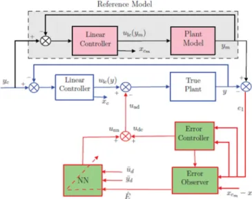
The Model Reference Adaptive Control scheme concept based on Single Hidden Layer Neural Network (SHLNN) and output feedback [1] is given in Fig 1.
Figure 1: Control architecture concept
The reduced order reference model is designed to possess the main dynamic of the system while the unmodeled dynamics, including flexibility, are assumed to act as disturbances to this model. The plant model is the full order model including sensor and actuator dynamics. The linear controller is designed to meet the performance specifications of the reference model. The adaptive signal uad, which augments the linear signal ulc, is generated using neural networks based on the error vector Ê, defined by the error observer. The augmented neural adaptation forces the plant model output y to be same as the reference model output ym.
In general, the closed loop reference model can be written similar to [1] & [2] as.
m m m c m m m X C y y B X A X = + = & (1)
The state vector XmT =[χmT zTm xTcm]is defined such that χm ,
zm and xcm are the state vectors of the reference model, the internal dynamicsand the linear controller respectively. In the augmentative approach, the adaptive signal defined by uad is simply augmented with the linear controller ulc as
u= ulc - uad (2) Thus the plant model could be written as
X C y u b y B X A X c ad = ∆ + − + = & (3)
with the definition of state vector [ 1 ] T c T T T x z X = χ is such
that χ is the state vector of the plant model, z1 is the state vector of internal dynamics, xc is the state vector of the linear controller. The uncertainties between the reference model and plant model are given by ∆T= [∆1T ∆2T 0], where ∆1T and ∆2T
are matched and unmatched uncertainties respectively. With yc being the reference input, the error vector e1 is the difference between the reference model output ym and plant output y. The error dynamics could be written from (1) and (3) as follows
(
)
E C z B u b E A E ad = ∆ − ∆ − + = 1 2 & (4)with state vector
[
T]
c cm T m T m T z z x x E = (χ −χ) ( − 1) ( − )
where the output vector z represents the signals available for feedback i.e the difference in outputs ym-y and states of linear controller, xcm-x. z= − − c cm m x x y y (5)
The studies in [1], [3] and [5] demonstrated that the matched uncertainty can be estimated with arbitrary accuracy ε* approximated using a single hidden layer neural network defined by ∆ = Tσ
( )
Tη +ε( )
η N M 1 ,( )
* ε η ε ≤ (6) with the definition of M and N being bounded constant weights of input and output layers of NN and σ being the activation function. The ε(η) is the neural reconstruction error with ηbeing the network input vector defined by finite history of input and outputs given by
( )
[
( )
T( )
]
T d T d t y t u t =1η
(7)The adaptive signal is designed as in [3]
( )
ησ T T
nn M N
u = ˆ ˆ (8)
whose weights are adapted online using the adaptation laws as given in [5]
[
(
)
]
[
E PbM kN]
N M k b P E N M T T N T T M ˆ ' ˆ ˆ ˆ ˆ ˆ ˆ ˆ ' ˆ ˆ ˆ + Γ − = + − Γ − = σ η η σ σ & & (9) in which N M ΓΓ , are positive adaptation gain matrices, k is the σ modification constant. σ σ
( )
Tη Nˆ ˆ= and( )
η σ σ T N d d ˆ ' ˆ = is theJacobian computed at the estimates in (9).
The adaptive signal is designed to stabilize the error dynamics defined in (4) which can be written as a linear error observer as
(
z CE)
K E A Eˆ& = ˆ+ − ˆ (10) whose gain K can be designed so that A−KCis stable and the observer having higher bandwidth than A.In general, the adaptive signal is defined together with an additive training signal udc for better command tracking and robustness to perturbations.
uad=unn+udc (11) The additive controller could be an optimal, modal or frequential controller. The error observer in (10) could be rewritten including (11).
III. EXPERIMENTAL VALIDATION
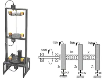
The experimental validation of the control scheme [1] is done on a three disk torsion pendulum [11]. The experimental setup and schematic of the model are shown in Fig 2.
Figure 2: Three disk torsion pendulum and schematic of the experiment For the sake of brevity, only the system parameters and results will be discussed. The objective is to control the bottom disk angular position (θ3), acting on the input voltage of a brushless DC motor (u). The reference model only contains the rigid dynamics and is defined by:
m m m m m m m x C y u B x A x = + = & (12) whose parameters are given by,
= 3 3
θ
θ
& m x , = 667 . 1 0 1 0 m A , = 65 0 m B = 0 1 m C (13)The linear controller is designed as a lead compensator, the error observer is defined similar to [1] with the definition of
error vector
[
]
c cm m m T x xE = θ3 −θ3 θ&3 −θ&3 − . The SHLNN is introduced to approximate the uncertainty ∆1. We use 8 delayed values of output θ3, 7 delayed values of input, u and
10 hidden layer neurons. The error vector has been used to change the adaptation online with the following adaptation parameters of ΓM =3000, ΓN=3000and k=0.15.
A. Results
It can be seen from Fig 3 that the tracking performance of the plant has been considerably improved upon adaptation for a step input of 20°. Except for a brief transient effect due to stiction, the output of the plant with adaptive signal uad represented in magenta tracks the ideal reference model output given in blue.
Figure 3: Output Response of Bottom Disk for a 20° Step Command The disturbance rejection performance has been performed with yc=0 and a disturbing non collocated input as in [1].
Figure 4: Output Response of Bottom Disk to Disturbances.
One of the major interests in adaptation is the robustness to parametric uncertainties of the plant. Experiments were done using different mass configurations on the lower disk to quantify the robustness of the adaptive controller to changing inertias which was designed without mass at the bottom disk. Fig 5 shows the tracking error with respect to reference model output, and the good robustness of the controller to parametric uncertainties could be seen with the acceptable bounds in tracking error with the maximum of ± 0.15 °.
Figure 5: Robustness to Parametric Uncertainties represented by tracking error with respect to reference model for various inertia cases.
The experimental validation of the control scheme yields promising results and the methodology could be extended to higher order complex systems such as aircrafts. Apart from performance tracking and disturbance rejection, the robustness to uncertainties is of interest in the flexible aircraft problem which involves higher parametric uncertainties such as inertia changes and non-parametric uncertainties such as gust, wind etc.
IV. FLEXIBLE AIRCRAFT PROBLEM
The longitudinal aircraft model used in the study is a linear state space model corresponding to different Mach numbers and center of gravity (CG) configurations depending on the weight of fuel tank. It is a 193 state model with 7 inputs of IA (Inner Aileron), OA (Outer Aileron), Elevator and wind respectively. The model has 105 outputs of which, angle of attack ∝, pitch rate q, pitch angle θ, vertical velocity Vz and vertical acceleration measure Nz are of interest to the present study. Since the measures are made at CG whereas, the problem is to control flexible modes, additional acceleration measures are made at right and left wings [2]. A linear combination of acceleration measures built to account for structural flexibility and passenger comfort is as follows
CG L R law Nz Nz Nz Nz = + − 2 (14) Where NzCG, NzR, NzL represents the vertical acceleration measures made at CG, right and left wings respectively [2].
0 1 2 3 4 5 6 7 8 9 10 -5 0 5 10 15 20 25 30 Time (s) y (d e g ) ideal No adaptation Udc Unn+Udc 0 1 2 3 4 5 6 7 8 9 10 -30 -20 -10 0 10 20 30 Time (s) y (d e g ) With adaptation Without adaptation 0 0.5 1 1.5 2 2.5 3 3.5 4 4.5 5 -0.4 -0.2 0 0.2 0.4 0.6 0.8 1 1.2 Time (s) T ra c k in g e rr o r( d e g ) No mass Bottom-2 mass Bottom-4 mass
The control objective is to reduce the oscillations defined by (14) either due to command or wind disturbances of the aircraft using IA as control variable.
Simulation of actuators includes typical nonlinearities like rate limiters and saturations. The bandwidths are approximately 27rd/s for the inner aileron, 10rd/s for the outer aileron and 25rd/s for the elevator. The measures are simulated using low-pass filters with a 3Hz bandwidth plus a pure delay of 160ms. The wind turbulence input is simulated using a white noise passing through a Von Karman filter.
A. Control Methodology
In designing the reference model adaptive control, the reference model has to be simple and includes main dynamic of the actual plant. In the study, the reference model is the rigid state space model of order 2 with outputs ∝ and q without sensor and actuator limitations. The linear controller is designed as an eigen structure controller, a commonly used control methodology in flight control domain. The linear controller could be a LQ/LQG or lead/lag controller also, but Modal approach is classical aircraft control design approach and hence retained here. The study is done for two different linear controllers which excite only the first flexible mode of 1.2 Hz, and the other controller excites both first and second flexible mode of 1.2 Hz and 2.7Hz, hitherto called as low frequency and high frequency mode respectively. The effectiveness of adaptation in reducing those two flexible modes of the aircraft is then studied. It may be noted that the first structural mode with low frequency is related to rigid control excitation and the second mode is related to the passenger comfort. It can be seen that we deal with Non collocated problem since our control objective is to reduce oscillations i,e Nzlaw, though state feedback is used. In addition, the plant model coupled with actuator model is a nonminimum phase system.
B. High Frequency Mode Control
An eigen structure controller has been designed for the rigid aircraft reference model with ω=2.03 rad/sand damping ratio δ=0.8 along with the pre command.
The plant model has same linear controller and pre command. The error observer described in (10) is designed as a first order filter. The adaptive signal unn is generated using three hidden layer neurons, nine delayed values of command u and eight delayed values of plant output y with sampling period of 2ms. The adaptation gains are chosen as ГM=0.5, ГN=0.5 and
learning rate modification constant k=2. The additive signal udc to train the NN is designed as an optimal LQR controller seeking to minimize quadratic criteria
J
(
Q Ru)
dt dc e T e∫
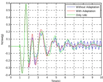
∞ + = 0 2 χ χ (15) with the weighing terms, Q=[4000 0.1] and R=20.The output response of the system for a step angle of attack (AoA) input of 1° is given in Fig 6. The adapted output is shown in red and it can be compared without adaptation shown in blue to see the effect of adaptation in controlling high frequency modes. The adaptive signal, uad i,e unn+udc, attenuates the second flexible mode of 2.7 Hz though there is
no action on first flexible mode of 1.2 Hz. The results with only udc is given in green for comparison.
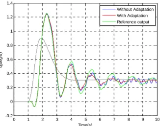
The output tracking of the controller is given in Fig 7. The effect of adaptation is not visible in ∝ tracking but could be seen in the attenuation of high frequency second mode in Fig 8 of pitch rate q evolution.
Figure 6: Nzlaw output response of aircraft model for 1° step AoA input
A measurable control quantity has been proposed by an energy criteria [2] defined by
∫
= t Nzlawdt t C 0 2 ) ( (16)The energy criteria evolution with adaptation is much better than without adaptation and it can be seen from Fig 9.
Figure 7: Angle of attack response of aircraft for 1° step AoA input The robustness to disturbance of adaptation is studied by setting the command, yc=0 and using the wind disturbance instead for a duration of 100s. In terms of vertical acceleration reduction due to wind gust alone, the adaptation yields better although not significant results in Fig 10.
0 1 2 3 4 5 6 7 8 9 10 -0.4 -0.3 -0.2 -0.1 0 0.1 0.2 0.3 0.4 0.5 0.6 Time(s) N z la w (g ) Without Adaptation With Adaptation Only Udc 0 1 2 3 4 5 6 7 8 9 10 -0.2 0 0.2 0.4 0.6 0.8 1 1.2 Time(s) a lp h a (d e g ) Without Adaptation With Adaptation Reference output
Figure 8: Pitch rate response of aircraft for 1° step AoA input
Figure 9: Control command energy criteria evolution for 1° step AoA
Figure 10: Control command energy criteria evolution for wind gust
C. Low Frequency Mode Control
The linear controller is designed for the rigid model with the specifications of ω=1.35 rad/sand δ=0.7 along with the pre command. The error observer is retained the same. The tuning of neural part has been carried out such that the number of neurons and the learning rate ГM, ГN were the same as
described in the previous section. The only difference being the learning rate modification constant, k=72 and the additive signal whose weighing parameters are Q= [10 10] and R=16.
The time domain simulation of the model carried out with a step AoA input of 1° is given in Fig 11.
Figure 11: Nzlaw output response of aircraft model for 1° step AoA input
The oscillations due to first flexible mode are seen to be reduced though there is a slight, but negligible spillover of second flexible mode. Though there is no tangible effect of adaptation in input command tracking similar to Fig 7, the effect of neural signal on reducing lower frequency flexible mode of 1.2Hz could be seen in pitch rate evolution shown in Fig 12.
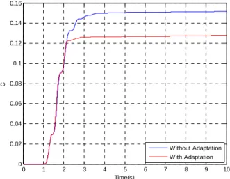
Figure 12: Pitch rate response of aircraft for 1° step AoA input The energy evolution criteria of command (16) is given in Fig 13, where the adaptation shown in red mitigates the total
0 1 2 3 4 5 6 7 8 9 10 -0.2 0 0.2 0.4 0.6 0.8 1 1.2 1.4 Time(s) q (d e g /s ) Without Adaptation With Adaptation Reference output 0 5 10 15 20 25 30 0 0.1 0.2 0.3 0.4 0.5 0.6 0.7 0.8 Time(s) C Without Adaptation With Adaptation 0 10 20 30 40 50 60 70 80 90 100 0 5 10 15 20 25 30 35 40 Time(s) C Without Adaptation With Adaptation 0 1 2 3 4 5 6 7 8 9 10 -0.8 -0.6 -0.4 -0.2 0 0.2 0.4 0.6 Time(s) N z la w (g ) Without Adaptation With Adaptation 0 1 2 3 4 5 6 7 8 9 10 -0.2 0 0.2 0.4 0.6 0.8 1 1.2 Time(s) q (d e g /s ) Without Adaptation With Adaptation Reference output
energy of the oscillations sustained due to flexible effects when compared against without adaptation case shown in blue.
The acceleration response to wind gust in the presence of disturbance given in Fig 14 shows higher command energy for adaptation due to persistent spillover of higher flexible mode due to gust for the duration of 100s. This could be alleviated at the expense of attenuation of the low frequency flexible mode. In fact, the adaptation is not tuned here for disturbance rejection performance, but rather for mitigation of specific first flexible mode with good command tracking.
Figure 13: Control command energy criteria evolution for 1° step AoA
Figure 14: Control command energy criteria evolution for wind gust The studies by [3] and [5] showed that there exists many degrees of freedom in tuning the adaptive parameters and it was always possible to find a set of tuning parameters to improve the control performance of a system. In the application to aircraft control, the present study attempts to improve the conclusions of [2], and demonstrates this adaptive ability for the control of different flexible modes while retaining the simplicity of reference model. A small scale of
network for adaptation, basic error controller and simple rigid reference model as the one described here could be of importance in case of future real time applications.
V. CONCLUSION
The application of adaptive output feedback augmentation to full order flexible aircraft using a simple rigid reference model showed that the adaptive part can be tuned depending on the mode to be controlled and linear controller design. This is in contrast to the classical method of using dedicated filters to control each flexible mode. The reference model chosen is a rigid model which is simple and it was shown that promising results could be obtained even using a simple model to control flexibility of a highly complex model. Though it may not be able to control all the frequency modes for a given controller configuration, nevertheless the scheme offers a different paradigm in controlling particular frequency modes depending on the choice of linear controller. A systemic approach to the choice of reference model and extension of the study to the robustness to parametric uncertainties such as its application for an aircraft LPV model could be made to demonstrate the effectiveness of the approach in aerospace control domain.
REFERENCES
[1] B.-J. Yang, N. Hovakimyan, A.J. Calise, J.I. Craig “Experimental Validation of an Augmenting Approach to Adaptive Control of Uncertain Nonlinear Systems” AIAA Guidance, Navigation and Control
Conference, number AIAA-2003-5715
[2] J. Bordeneuve-Guibe, L. Bako, M. Jeanneau “Adaptive output feedback control based on neural networks:application to flexible aircraft control”
The 2nd IFAC International Conference on Intelligent Control Systems and Signal Processing, 21-23 Sept 2009, Istanbul, Turkey.
[3] B.-J. Yang “Adaptive Output feedback Control of Flexible Systems”
Thesis School of Aerospace Engineering, Georgia Institute of T.echnology, 2004, Unpublished.
[4] N. Kim “Improved Methods in Neural Network-Based Adaptive Output feedback Control, with Applications to Flight Control” Thesis School of
Aerospace Engineering, Georgia Institute of Technology, 2003,
Unpublished.
[5] N. Hovakimyan, B.-J. Yang, A.J. Calise “An Adaptive Output Feedback Control Methodology for Non-Minimum Phase Systems” Conference on
Decision and Control, Las Vegas, NV, pp 949-954, 2002.
[6] M. Jeanneau “Commande Active de Structures Flexibles : Applications Spatiales et Aéronautiques”, Notes de Cours Supaéro, Course Notes of Supaero, Toulouse, 2000, Unpublished.
[7] A. Isidori “Nonlinear Control Systems” Springer Verlag London Ltd. 1995.
[8] J. Bordeneuve-Guibé, L. Bako, M. Jeanneau “Amortissement des modes de flexion voilure: utilisation d'une commande adaptative en boucle fermée”. Journal Européen des Systèmes Automatisés, 2011. ISSN 1269-6935, pp 513-529, Vol 45-n° 7-8-9-10/2011.
[9] P.R. Pagilla, B. Yu, K.L. Pau “Adaptive Control of Time-Varying Mechanical Systems: Analysis and Experiments” IEEE,Transactions on
Mechatronics, vol. 5, n° 4, dec 2000.
[10] I.D. Landau “From Robust to Adaptive Control” Control Engineering
Practice 7 1113-1124, 1999.
[11] “Torsion Pendulum Appratus, ECP Systems, Inc.” http://www.ecpsystems.com/controls/torplant.html. 0 1 2 3 4 5 6 7 8 9 10 0 0.02 0.04 0.06 0.08 0.1 0.12 0.14 0.16 Time(s) C Without Adaptation With Adaptation 0 10 20 30 40 50 60 70 80 90 100 0 5 10 15 20 25 30 35 40 45 Time(s) C Without Adaptation With Adaptation