FPGA-BASED COMPUTATION OF THE INDUCTANCE OF COILS USED FOR THE MAGNETIC STIMULATION OF THE NERVOUS SYSTEM

HAL Id: ensl-00169909

https://hal-ens-lyon.archives-ouvertes.fr/ensl-00169909

Preprint submitted on 11 Sep 2007

HAL is a multi-disciplinary open access

archive for the deposit and dissemination of

sci-entific research documents, whether they are

pub-lished or not. The documents may come from

teaching and research institutions in France or

abroad, or from public or private research centers.

L’archive ouverte pluridisciplinaire HAL, est

destinée au dépôt et à la diffusion de documents

scientifiques de niveau recherche, publiés ou non,

émanant des établissements d’enseignement et de

recherche français ou étrangers, des laboratoires

publics ou privés.

FPGA-BASED COMPUTATION OF THE

INDUCTANCE OF COILS USED FOR THE

MAGNETIC STIMULATION OF THE NERVOUS

SYSTEM

Ionuţ Trestian, Octavian Creţ, Laura Creţ, Lucia Văcariu, Radu Tudoran,

Florent de Dinechin

To cite this version:

Ionuţ Trestian, Octavian Creţ, Laura Creţ, Lucia Văcariu, Radu Tudoran, et al.. FPGA-BASED

COMPUTATION OF THE INDUCTANCE OF COILS USED FOR THE MAGNETIC

STIMULA-TION OF THE NERVOUS SYSTEM. 2007. �ensl-00169909�

FPGA-BASED COMPUTATION OF THE INDUCTANCE OF COILS USED FOR THE

MAGNETIC STIMULATION OF THE NERVOUS SYSTEM

Ionuţ Trestian, Octavian Creţ, Laura Creţ,

Lucia Văcariu, Radu Tudoran

Computer Science Department

Technical University of Cluj-Napoca

26 Bariţiu street, Cluj-Napoca, Romania

email: Octavian.Cret@cs.utcluj.ro

Florent de Dinechin

LIP, Ecole Normale Supérieure de Lyon

UMR CNRS/INRIA/ENS-Lyon/Université

Claude Bernard Lyon 1

46 allée d'Italie, 69364 Lyon cedex 07, France

email: Florent.de.Dinechin@ens-lyon.org

ABSTRACT

In the last years the interest for magnetic stimulation of the human nervous tissue has increased considerably, because this technique has proved its utility and applicability both as a diagnostic and as a treatment instrument. Research in this domain is aimed at removing some of the disadvantages of the technique: the lack of focalization of the stimulated region and the reduced efficiency of the energetic transfer from the stimulating coil to the tissue. Better stimulation coils can solve these problems. Designing coils is so far a trial-and error process, relying on very compute-intensive simulations. In software, such a simulation has a very high running time (several hours for complicated geometries of the coils). This paper proposes and demonstrates an FPGA-based hardware implementation of this simulation which reduces the computation time by 4 orders of magnitude. Thanks to this powerful tool, some significant improvements in the design of the coils have already been obtained.

1. INTRODUCTION

The preoccupation for improving the quality of life, for persons with different handicaps, led to extended research in the area of functional stimulation. Due to its advantages compared to electrical stimulation, magnetic stimulation of the human nervous system is now a common technique in modern medicine [1].

A difficulty of this technique is the need for accurate focal stimulation. Another one is the low efficiency of power transfer from the coil to the tissue. To address these difficulties, coils with special geometries must be designed.

Because of the diversity of the medical applications involved, the design of the coils requires testing a large number of geometries in order to find an adequate solution for the desired application [2].

One of the major problems that appear in the design phase of such coils is the computation of the inductivity of the stimulating coil. For simple shapes of the coils (circular), one can determine analytical computation formulas [3] which are extremely complicated. When, however, the shape and the spatial distribution of the coil’s turns do not belong to one of the known structures, a numerical method needs to be used for determining the inductivity of the coils.

The idea of the computation method is to divide the coils in small portions. Starting from this method, two computation systems are presented in the paper:

• The first one is classical and it just consists of a software implementation (Matlab);

• The second one consists of realizing a hardware architecture that exploits the intrinsic parallelism of the problem. The physical support of this architecture is an FPGA device.

The problem with the software implementation is its running time. Coils are designed by trial-and-error, and this approach is impractical if each trial requires half a day of computation. Besides, as this time grows with the complexity of the coil, it prevents designing complex coils. This paper shows that FPGA-based hardware acceleration is able to solve this bottleneck.

The rest of the paper is organized as follows: Section 2 briefly presents the inductivity computation process. In section 3 some considerations are made about the software implementation. Section 4 deals with the hardware implementation and presents the global architecture as well as the architecture of the main building blocks. Section 5 makes a comparison between the two implementations in terms of running speed and results obtained, and Section 6 presents the main conclusions of this work.

2. INDUCTIVITY COMPUTATION

The simulation of magnetic stimulators with complex forms requires dividing their coils in several parts. The self-inductance of the circuit, divided in n parts, can be

computed with formula (1). This mainly adds up the self-inductivities of the separate segments with the mutual inductivities of all the involved segments. The method is described in [4] and in more detail in [5].

(

i k

)

for M L L n k n i ki n k k+ ≠ =

∑

∑∑

= = = , 1 1 1 (1)

The self-inductivity of a short straight conductor, with round cross-section, for low frequencies, is given below:

      − + − = ₂ 2 0 4 45 128 4 3 2 ln 2 l r l r r l l L π π µ (2)

where l is the conductor’s length, and r the radius of its cross-section. The mutual inductivity between two straight conductors converging into a point is evaluated as:

      − + + + + − + + + ϕ π µ = a b c c b a ln b b a c c b a ln a cos M 4 0 (3)

The given quantities are represented in Figure 1, with a and b representing the length of the conductors, andφ the angle between them.

a

b c

ϕ

Fig. 1. Computing the mutual inductivity between two converging conductors

For the general case, we consider two conductor segments in space. The first segment is delimited by the points of coordinates (xa, ya, za) and (xb, yb, zb), while the

second segment is delimited by the points of coordinates (xc, yc, zc) and (xd, yd, zd), as shown in Figure 2.

1 Γ (xa,ya,za) r l1− 1 l (xb,yb,zb) (x,y,z) (xd,yd,zd) (xc,yc,zc) r Γ2 l2

Fig. 2. Two segments in space

On the second segment, we consider a point of coordinates (x, y, z). The parametric equation of the second segment is:

(

)

(

)

(

)

     − + = − + = − + = t z z z z t y y y y t x x x x c d c c d c c d c (4)

With the above geometrical coordinates, we can find the

mutual inductivity between these segments (using

Neumann formula). For two circuits, Γ1 and Γ2, in a

homogenous media with µ permeability, the mutual

magnetic fluxΦ21is:

∫

∫

Γ Γ = = Φ 2 2 2 21 21 21 S dl A dS B (5)

Since circuits Γ1 and Γ2 are shaped like two straight

segments, the mutual flux can be evaluated by integrating the magnetic vector potential created by the first segment along the second one. Considering the magnetic vector potential generated by a conducting segment, the mutual inductivity can be computed using the following equation:

∫

Γ ⋅ ⋅ ⋅ − ⋅ − + − ⋅ = 2 2 1 1 1 1 1 1 1 1 0 21 ₄ ln _l dl l l r l r l r l l r l L π µ (6)

The vectors in equation (6) are:

( )

( )

( )

(

)

(

)

(

)

(

)

(

x x i y y j z z k

)

dt; dt k t ' z j t ' y i t ' x dl d c d c d c− ⋅ + − ⋅ + − ⋅ ⋅ = = ⋅ ⋅ + ⋅ + ⋅ = 2

( )

( )

( )

(

)

(

)

(

)

(

)

(

x x i y y j z z k

)

dt; dt k t ' z j t ' y i t ' x dl d c d c d c− ⋅ + − ⋅ + − ⋅ ⋅ = = ⋅ ⋅ + ⋅ + ⋅ = 2

(

x x

)

i

(

y y

)

j

(

z z

)

k l1= _b− _a ⋅ + _b− _a ⋅ + _b− _a ⋅ ;

(

x x

)

i

(

y y

)

j

(

z z

)

k r= − _a ⋅ + − _a ⋅ + − _a ⋅ ;

(

x x

)

i

(

y y

)

j

(

z z

)

k r l1− = _b − ⋅ + _b − ⋅ + _b − ⋅ ; (7)

while coordinates x, y, z are expressed as a function of parameter t, according to (4). The limits of the integral in equation (6) are given by t

∈

[0, 1].

As can be seen in the above formulas, the operations involved in computing the inductivity of a coil are vector operations. A logarithm, some division, addition and multiplication operations can also be observed in equation (6). Equation (1) is mainly an accumulation of mutual inductivities. The integral according to t will be evaluated using the trapezoidal method.

3. SOFTWARE IMPLEMENTATION

A coil is made up of a certain number of turns rolled around a central rod. Each turn can be considered as a perfect circle. The coil is structured on several vertical stages. On each stage there are more turns (horizontal turns). The outer radius of the coil will be further denoted by a. Other parameters are the diameter of the metallic turn and the distance (insulation) between consecutive turns.

Fig. 3. Coil approximation using a finite number of points

It is possible to have a different number of turns on every vertical stage. It is also possible to have a variable number of vertical stages, as shown in Figure 3, where one can also notice the different number of turns on each stage.

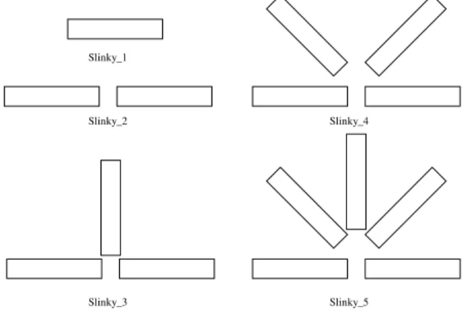
A complete magnetic stimulation device contains a Slinky coil. Considering a coil with N turns, the “Slinky-k” coil is generated by spatially locating these turns at successive angles of ix180/

(

k−1

)

degrees, were i = 0, 1, …, k-1. If the current passing through this coil is I, then the central leg carries the total current N x I. These coils are shown in Figure 4, where each rectangle represents a leaf of the coil, viewed in perspective.

Slinky_1

Slinky_2

Slinky_3

Slinky_4

Slinky_5

Fig. 4. Magnetic coil structures of the stimulation device For computing the inductance, the turns could be approximated by a finite number of points. We considered, after a series of tests, that a suitable amount of points on a turn is 64.

We therefore need to compute the inductance of such a coil. We have to take each of the 64 points and combine them into segments made up of one point and the next (consecutive) point in a certain direction. After this, each segment, one by one, is held as a reference. Then, the formula presented in this paragraph is applied using this reference segment and all the other segments on the coil.

For each pair of segments a value is obtained. These values must be added in order to obtain the coil’s total inductance.

There are two phases for the functioning of the software implementation:

• In Phase 1, the coordinates of the points are generated. These are computed using trigonometric functions. The results produced in this phase are also used in the hardware implementation.

• In Phase 2, the actual computation of the values is performed. As mentioned before, in order to compute the inductivity, we accumulate the values corresponding to the mutual inductivities.

When we evaluate pairs of segments on the coil, three distinct cases can arise:

• The two segments are actually the same segment. In this case we add the segment’s own self-inductivity given by Equation (2). Since all segments have the same characteristics, this value is the same for all segments.

• The two segments are neighboring segments, that is, they have exactly one common point. In this case their mutual inductivity is given by Equation (3). Since the configuration is the same for all pairs of neighboring segments, this too is a constant value.

• The two segments are neither the same nor neighboring; they are two distinct segments in space. For complex configurations consisting of a large number of turns, this is the most general case, which accounts for most of the computation time. This case is evaluated using Equation (4). The software implementation takes into account these considerations. We evaluate the third case by computing the mutual inductivities of all non-intersecting segments. The self-inductivity of the segments and the mutual inductivities of each segment against its neighboring ones are multiplied by the number of segments and accumulated at the end.

In order to evaluate the mutual inductivity of two separate segments in space we have introduced 5 variables denoted var1to var5which correspond to vector operations involving the two segments as described in the previous section. These variables will also be used in the next section. The points (x0, y0, z0) and (x1, y1, z1) correspond to

the extremities of the first segment, while (x2, y2, z2) and

(x3, y3, z3) correspond to the extremities of the second one.

) ( ) ( ) ( ) ( ) ( ) ( var₁= x₁−x₀ ⋅x₃−x₂ + y₁−y₀ ⋅ y₃−y₂ + z₁−z₀ ⋅z₃−z₂ 2 2 3 2 2 3 2 2 3 2 ( ) ( ) ( ) var = x−x + y −y + z −z 2 1 0 0 3 2 1 0 0 3 2 1 0 0 3 3 (( ) ( ) ) (( ) ( ) ) (( ) ( ) ) var= x−x + x−x ⋅t + y −y + y−y ⋅t + z −z + z −z ⋅t 2 2 0 1 0 2 2 0 1 0 2 2 0 1 0 4 ( ( ) ) ( ( ) ) ( ( ) ) var = x +x −x ⋅t−x + y + y −y ⋅t−y + z + z −z ⋅t−z + − ⋅ − + ⋅ − + − ⋅ − + ⋅ − =( ) ( ( ) ) ( ) ( ( ) ) var5 x3 x2 x0 x1 x0 t x2 y3 y2 y0 y1 y0 t y2 ) ) ( ( ) (z3−z2 ⋅z0+ z1−z0 ⋅t−z2

These values are used for further computing the accumulation value: 2 5 4 2 5 2 3 2 1 var var var var var var var log var var r Accumulato r Accumulato − − + ⋅ + = (8)

In the formulas above there is a variable t, which is a factor occurring in the integral from Equation (6). Therefore several values need to be considered for t and then the integral needs to be computed using the trapezoidal method for values in the interval (0, 1) = [0.1, 0.2, 0.3 … 0.9]. The process above needs to be repeated several times in order to compute the final inductivity of the coil.

The main drawback of a software implementation is the extremely high running time. It can be in the order of tens of minutes even for simple configurations, while for complex geometries of the coils it can exceed several hours (Ex: for a 58-turns coil, about 5 hours computation time on a recent PC).

Once the software simulation had been validated against actual coils, it was decided to try to accelerate it using custom hardware.

4. HARDWARE IMPLEMENTATION 4.1. Field-programmable gate arrays

A Field-Programmable Gate Array (FPGA) is a semiconductor device containing programmable logic components (“logic blocks”), and programmable interconnects. Logic blocks can be programmed to perform simple or more complex functions. In most FPGAs, the logic blocks also include memory elements, from flip-flops to more complete blocks of memories.

A hierarchy of programmable interconnects allows logic blocks to be interconnected as needed by the system designer, somewhat like a one-chip programmable breadboard. Logic blocks and interconnects can be programmed by the customer/designer, after the FPGA is manufactured, to implement any logical function. Their advantages include a shorter time to market, ability to re-program in the field to fix bugs, and lower non-recurring engineering costs [6].

4.2. Floating point operators - FPLibrary

Several libraries of floating-point operators for FPGAs have been published in the last few years. In this work, we use FPLibrary, developed at Ecole Normale Supérieure de Lyon and freely downloadable from [7]. Mantissa size and exponent size parameterize each operator in this library, allowing one to choose the precision and the dynamic range of the numbers. It provides operators for addition, subtraction, multiplication, division and square root, some useful conversions and some elementary functions

(currently exponential, logarithm and sine/cosine), in combinatorial or pipelined flavor. It is written in portable VHDL. FPLibrary also offers operators for the alternative

logarithmic number system[8].

The Core Generator tool, which comes with the Xilinx ISE, also offers floating-point operators. FPLibrary was chosen essentially because it offers a logarithm [9] which is not available in the Core Generator. However, it also proved more area-efficient. As our design requires a large number of operators in a tree-like pipeline, latency was not our main concern.

4.3. System architecture

The hardware implementation implies the same two phases as the software one, but Phase 1 is not computation-intensive and its implementation is kept in software.

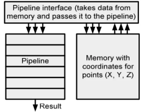
In the Figure 5 below a block diagram of the system is displayed. Three main blocks can be distinguished. The most important block is the pipeline stage, which receives values, computes them, and in a final stage accumulates them. The pipeline will be described afterwards.

Fig. 5. Architecture of the hardware system The coordinates are stored in a Block RAM memory. There are 3 memories, one for each coordinate, X, Y, and Z. The synchronization logic, which gives the data to the pipeline, is implemented in a special interface. This interface consists of counters and latches. The counters are orchestrated to generate the proper addresses, while the latches are needed to implement a caching logic, which saves some of the memory used.

The pipeline stage consists of several sub-stages, based on the computations involved:

• ••

• A first stage computes the variables var1, var2, var3,

var4 and var5 (the formulas were given in the

previous section). There are several operations, which are common to the 5 variables. The pipeline reuses the corresponding intermediate values. •

••

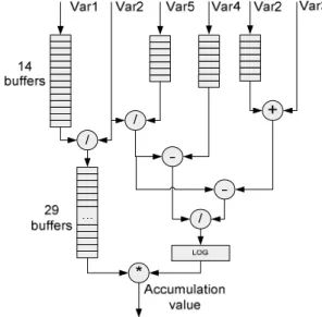
• The second stage computes the value to be accumulated and it is presented in Figure 6. The latencies in this part of the pipeline are pretty large,

up to 14 cycles, corresponding to waiting for a square root and about 29 cycles waiting for the logarithm and other operations to finish.

• ••

• The third stage is the accumulator. Because FPLibrary doesn’t provide such a component one needed to be improvised using the existing resources. Special considerations were made in order to work around the specific latency that a simple adder introduces.

Not only the specific operators, but also buffer stages are used, which compensate the latency introduced by some of the operators. For instance, the addition operator always introduces three cycles of latency and this must be compensated with three buffers. This also goes for the multiplication operator, which introduces four cycles of latency.

The design of the Accumulator is the most important part of the pipeline’s architecture, since it computes intermediary values and at the end provides the final result. As mentioned above, special considerations need to be made with regard to the accumulator because of the latencies introduced by the adders in the FPlibrary (3 cycles).

Fig. 6. Second stage. Computing accumulation value The values that will be accumulated come and enter the accumulator stage on the pin located to the left. The accumulator has a classical structure, using a feedback input. The process can be seen below in Figure 7.

N1 N2 N3 N4 N5 N6 N7 N8 N9 Input Output N1 N2 N3 N2 + N5 N1 + N4 N3 + N6 N1 + N4+ N7 N2 + N5+ N8 N3 + N6+ N9

Fig. 7. Adder latency issues

Input numbers come serially, N1, N2, N3, N4, etc. The

adder at the beginning of the accumulating stage adds these numbers. Because of the 3 cycles clock latency, when N1,

N2, N3 have been inserted in this adder, the next numbers

that come are to be added to the numbers that have been inserted 3 cycles before. For example N1is added with N4,

N5with N2and N6with N3respectively. The same goes for

the next numbers, N7, N8and N9.

All the numbers are added but at the end three sums are generated: one for the numbers N1, N4, N7… N3k+1, the next

for the numbers N2, N5, N8 …. N3k+2, and the last for the

numbers N3, N6, N9… N3k(as shown in Figure 8).

Fig. 8. Architecture of the accumulator

These three sums are added in the final stage of the accumulator to generate the exact result. This final stage consists of three registers that delay the three corresponding sums. We add these three registers together in order to generate the final result.

One idea regarding the accumulating stage of the computation is to keep the other stages in a Simple Precision Format (32 bits) and enhance only the accumulator (64 bits, or only with a larger mantissa). Such a design would greatly limit the error losses corresponding to the accumulation of numbers of different ranges.

4.4. Hardware implementation issues

The performance and feasibility of the hardware implementation largely depends on its physical support. Our hardware platform was a Digilent Inc. board populated with a Xilinx Virtex2PRO30 FPGA device. The problem with this implementation was that it is quite large: it depleted the space of the FPGA device we had available at this moment. To estimate the total space needed, we synthesized the design for a larger FPGA device (a Virtex4 160LX). A report of the device utilization is shown below:

Selected Device: 4vlx160ff1148-12

Number of Slices: 23656 out of 67584 35%

Number of Slice Flip Flops: 20834 out of 135168 15%

Number of 4 input LUTs: 44515 out of 135168 32%

The maximum frequency for this implementation was reported as 137.552MHz.

As we can see the implementation fits without problems on this Virtex4 board. Regarding an implementation on our Virtex2Pro board two options were available.

The first option was to reduce the precision at which the pipeline operated. This ensured a reduction of both the buffer stages that provided the synchronization between the stages and a reduction in size of the operators.

This option was first implemented. We reduced the mantissa of the operands by 10 bits. Instead of a large mantissa having 23 bits, the mantissa now had only 13 bits. Although the design fitted on a Virtex-II Pro board at about 98% of its capacity, the results obtained with this method were discouraging. They were more then 30% off from the actual result provided by Matlab. Therefore another method needed to be found.

The next option was to reduce the frequency at which the pipeline stage operates and time-multiplex some of the resources (square root – three occurrences in design, some of the adders). This has the advantage of preserving the pipeline’s precision, the cost being a reduction in speed.

Selected Device: 2vp30ff896-6

Number of Slices: 13380 out of 13696 97%

Number of Slice Flip Flops: 15350 out of 27392 56%

Number of 4 input LUTs: 24156 out of 27392 88%

Of course we have a reduction in operating frequency: 85.714 MHz related to the weaker characteristics of the FPGA device and the more precise timing requirements.

5. EXPERIMENTAL RESULTS

The main achievement of the hardware implementation over the software one is the reduction in computation time. By performing one accumulation per clock cycle the hardware solution is indeed efficient and can be used even for the most complex magnetic stimulation systems.

In terms of complexity, both implementations, in software and in hardware, have the same complexity, O(n2) with n being the number of distinct segments. As we have said the specific hardware structure performs one accumulation per clock cycle. That means that each clock cycle, a mutual inductivity between two segments is evaluated. The software implementation performs the same computations in a longer time.

We have analyzed our software and hardware implementations using three distinct configurations (Figure 9). The values produced by the implementations are given in Table 1, where we can see the comparison between the results provided by the software and the hardware solutions. At first we analyze simpler cases, 1 to 4 turns. The outer turns are the widest turns on the coil while the inner turns are the neighbors of the outer turns located closer to the center. Then the results for the given configurations are presented. The analyzed quantity was the inductivity. We give also the number of segments, which determines the complexity.

Fig. 9. Analyzed configurations

The results of the two methods analyzed for the three configurations mentioned always stayed in the range of 3-4% of each other, with the Matlab result being slightly bigger than the result given by the hardware implementation. This can be attributed to the fact that Matlab uses by default double precision while in our system we have used only single precision operations. Indeed, a rough worst-case error analysis tells us that the accumulation, in the largest coil test, of 10.1920² floating-point numbers introduces a cumulative rounding error that may invalidate up to log2(10.1920²) = 25 bits of the result,

when the mantissa of a single-precision number holds 24 bits only.

This is a worst-case situation: in an actual simulation, these rounding errors compensate each other, which explains that our results are still accurate. However, it shows that we will require increasing the precision of the floating-point format to use this architecture on larger coils. Fortunately, this extra precision is mostly useful in the final accumulator.

Table 1. Comparison of results Configuration Inductivity (Hardware) [µH] Inductivity (Software) [µH] Number of segments 1 outer turn 0.097 0.097 64 2 outer turns 0.30 0.30 128 4 turns (2 out. 2 in.) 0.92 0.93 256 Slinky_1 coil 3.81 3.9 640 Slinky_2 coil 8.4 8.6 1,280 Slinky_3 coil 13.32 13.6 1,920 The flexibility of FPGAs allows us to use different precisions in different parts of the architecture. Besides, a format intermediate between single and double precision

may be used. For us, a 32- or 36-bit mantissa would already be overkill (double-precision has a 53-bits mantissa). We will test this as soon as we get hold of a board with a larger FPGA than the Virtex-II used here. It should be noted that this more accurate pipeline will require more hardware, but the same execution time: it will still compute one accumulation per cycle.

Table 2. Comparison of results Configuration Duration (hardware) [no. of clock cycles] Running speed* (hardware) [seconds] Running speed (software) [seconds] 1 outer turn 40,960 0.00047 4.2 2 outer turns 163,840 0.00194 18 4 turns (2 out. 2 in.) 655,360 0.00764 72 Slinky_1 coil 4,096,000 0.04705 420 Slinky_2 coil 16,384,000 0.19411 1,680 Slinky_3 coil 36,864,000 0.42941 3,600 * at 85.714 MHz, clock period 11.66 ns

One can see from Table 2 that the software running time is very large. That is why software computation becomes prohibitive for large systems. The largest such system we have analyzed (a coil consisting of 58 turns) took nearly 5 hours to compute in software.

As a global comparison, the hardware solution runs approximately four orders of magnitude faster then the software one. The frequency is related to the physical board we had available, but for a more recent FPGA chip (i.e. Virtex4LX160, for which we did some simulations, or Virtex5), the device’s capacity as well as the working frequency will increase, thus leading to an improved performance.

6. CONCLUSIONS AND FUTURE WORK

The equipment used in magnetic stimulation of the nervous system is costly and bulky. This is mainly due to the fact that the currents flowing through the stimulation coil are very intense (kA), leading to coil heating and strong electromagnetic forces that might destroy the coil. Therefore, magnetic coil design is one of the most important aspects of the technique of magnetically stimulating the nervous system.

An adequate geometry of the coil can lead to a better focality of the stimulus (the ability of a coil to stimulate a small area of the tissue) and it can also improve the efficiency of the energy transfer from the coil to the target tissue. The form and size of the turns, their position inside the coil, the insulation gap between turns are all important parameters that should be considered when designing a magnetic coil. Therefore, in order to establish the most suitable coil geometry for a specific medical application, a

large number of structures have to be tested, making of coil design a trial-and-error process, even if the risk involved is only computation time.

In a very recent paper [10], we analyzed the influence that space distribution of the magnetic coils’ turns has on the efficiency of energy transfer from the stimulator to the target tissue. The analysis was performed for a Slinky_3 coil configuration (see Figure 9), with applications on transcranial magnetic stimulation (TMS). It turned out that the electrical energy dissipated in the circuit of the stimulator – required in order to achieve the activation threshold – is 25% lower for the most efficient configuration than for the less efficient one, and the coil heating per pulse is also 35% smaller!

This estimation was based on the inductivity calculus described in this paper, and the large number of analyzed structures required a less time-consuming computation technique, the hardware implementation described above.

Since every medical application requires its own optimal structure of the magnetic coil, the results emphasized in this paper can play an important role for future work on coil design.

Because of the large amount of operations involved (several tens of millions just for one coil) it is very hard to debug such a hardware system at least at an acceptable level, but the obtained results show an excellent concordance with those obtained in software. Our implementation has the advantage of greatly speeding up the computation time and hence shortening the design process. On larger FPGA devices the process can achieve a greater speed by accommodating more computational structures in parallel. These structures would evaluate multiple pairs of segments in parallel and accumulate them to the final value.

The architecture will still undergo some accuracy fine-tuning, and benefit from soon-to come improvements to FPLibrary, such as a combined norm operator or an optimized accumulator. An idea is to vary the working precision along the pipeline to increase the final accuracy. In particular, increasing the size of the mantissa of the final accumulator would reduce the rounding errors due to the accumulation.

The development of an optimized norm operator (to be included in FPLibrary) will provide a space efficient alternative to the combination of multipliers and adders we currently use in the implementation and would probably enhance the latency as well.

The next step of this research will consist of a study on 50 cases of coils with large numbers of turns (more than 70 turns, in the different configurations: Slinky_2, Slinky_3, Slinky_4 and Slinky_5). The powerful FPGA-based computational tool described in this paper allows us to compute both the coil’s inductivity and the magnetic field’s value on a given point in a short time (a few minutes, which is much less than the time that a software run would require

– remember that for a 58-turns coil, the necessary time is 5 hours, and the runtime grows in a quadratic fashion!).

7. REFERENCES

[1] D. Mozeg and E. Flak. “An Introduction to Transcranial

Magnetic Stimulation and Its Use in the Investigation and Treatment of Depression”. University of Toronto Medical Journal, vol. 76, no.3, 1999, pp. 158-162.

[2] Griškova1, I., Höppner, J. “Transcranial magnetic

stimulation: the method and application”. Medicina

(Kaunas) 2006; 42(10), pp. 792-804.

[3] K. S. Han. “Self-inductance of air-core circular coils with rectangular cross section”, IEEE Transactions on Magnetics, vol. 23, no. 6, November 1987, pp. 3916- 3921.

[4] L Creţ, R. Ciupa, “Remarks on the Optimal Design of Coils

for Magnetic Stimulation”, ISEM Proceedings, Bad Gastein, Austria., 2005, pp. 352-354.

[5] P. Kalantarov, L. Teitlin. “Calculul inductivităţilor”, Ed. Tehnică, Bucuresti, 1958.

[6] D. Guell, T. El-Ghazawi, K. Gaj, and V. Kindratenko.

“High-Performance Reconfigurable Computing”, IEEE

Computer, vol. 40, no. 3, March 2007, pp. 23-27.

[7] http://perso.ens-lyon.fr/jeremie.detrey/FPLibrary/

[8] S. Collange, J. Detrey, and F. de Dinechin. “Floating Point or LNS: Choosing the Right Arithmetic on an Application

Basis.” Proceedings of the 9thEUROMICRO Conference on

Digital System Design, Dubrovnik, Croatia, August 2006, pp. 197-203.

[9] J. Detrey, F. de Dinechin. “A Parameterizable Floating-Point Logarithm Operator for FPGAs”. Proceedings of the 39th Asilomar Conference on Signals, Systems & Computers, November 2005, pp. 1186 – 1190.

[10] L. Creţ, M. Pleşa, D. D. Micu and R. Ciupa. “Magnetic

Coils Design for Focal Stimulation of the Nervous System”, Proceedings of EUROCON 2007, IEEE International Conference on Computer as a Tool, 9-12 September 2007, Warsaw, Poland.