Multiobjective Optimization of Parallel Robots and Optimal Path Placement

HAL Id: tel-01390055

https://hal.archives-ouvertes.fr/tel-01390055

HAL is a multi-disciplinary open access archive for the deposit and dissemination of sci-entific research documents, whether they are pub-lished or not. The documents may come from teaching and research institutions in France or abroad, or from public or private research centers.

L’archive ouverte pluridisciplinaire HAL, est destinée au dépôt et à la diffusion de documents scientifiques de niveau recherche, publiés ou non, émanant des établissements d’enseignement et de recherche français ou étrangers, des laboratoires publics ou privés.

Optimal Path Placement

Raza Ur-Rehman

To cite this version:

Raza Ur-Rehman. Multiobjective Optimization of Parallel Robots and Optimal Path Placement. Robotics [cs.RO]. Ecole Centrale de Nantes (ECN), 2009. English. �tel-01390055�

Ecole Centrale de Nantes

É

D

SPIGA

Année 2009…….. N° B.U. : (laisser l’espace prévu ici)

Thèse de D

OCTORAT

Spécialité : MENTION DE LA SPÉCIALITÉ

Présentée et soutenue publiquement par :

UR-REHMAN Raza

le 17 décembre 2009 à Nantes

T

M

O

P

R

O

P

P

J

Président : ……… . M Vigen Arakélyan, Professeur, INSA, Rennes Rapporteurs : ………..

Examinateurs : ………

M Romdhane Lotfi, Professeur, Laboratoire de Génie Mécanique, Sousse M Zeghloul Saïd, Professeur, Laboratoire de Mécanique des Solides, Poitiers M Olivier Company, MCF LIRMM, LIRMM, Montpelier

M Philippe Wenger, Directeur de recherche, IRCCyN, Nantes M Chablat Damien, Chargé de recherche HDR, IRCCyN, Nantes M Caro Stéphane, Chargé de recherche, IRCCyN, Nantes

Directeur de thèse : Philippe Wenger Laboratoire : IRCCyN

Co-directeur : D. Chablat Co-encadrant : S. Caro

1

Acknowledgment

On conclusion of three years of research work at IRCCyN, I am indebted in gratitude to The Almighty and my colleagues, whose contribution in this research in assorted ways has realised this dream. During this time, I have worked with many people and it is a pleasure to convey my gratitude to them in my humble acknowledgment.

In the first place I would like to express my gratitude to my thesis director Philippe Wenger for his guidance and valuable advices throughout this research work as well as his support in all other affairs.

I gratefully acknowledge my supervisor Damien Chablat for his supervision and important contributions. His sincere involvement with his originality has fostered my intellectual maturity that I regard as a lifetime asset. I am obliged for this generosity and wish to have collaboration in future as well.

Many thanks go to my co-supervisor St´ephane Caro whose close supervision, guidance and support enabled me to develop an understanding of the subject. His wise comments helped me to excel in generation and presentation of results and also progress as a student, a researcher and a scientist. He also put me on the road to LA_{TEX for my publications} and thesis report, thanks to which I succeeded to have encouraging remarks from the jury members. Thanks St´ephane!

The work presented in this dissertation was supported in part by the Higher Education Commission (HEC), Government of Pakistan. Thanks should also be extended to the HEC and particularly to the Ex-Chairman HEC, Dr. Atta-ur-Rehman founder of this research program.

On a personal note, I would like to thank my friends and colleagues in Pakistan and in France for their prayers, encouragements and concerns, particularly my best friend Shafqat Waqar Ahmad for his tireless help for all of my matters in Pakistan. Here in Nantes, I have been blessed with a friendly and cheerful group of fellows. Their company made my stay memorable and lessened the work stress and gave me a support in my good and bad times. Thanks buddies!

boundless, my sisters, my brothers and especially my father, who is no longer with us, as he used to be the happiest person on earth on my any accomplishment. Special thanks go to my parents-in-law and my wife who suffered a three years forced-separation (probably forced by French Embassy in Pakistan) right after our marriage because of French visa problem. Her love, understanding, patience and support are the most important things to me. Love to my two-year old daughter, Simaal Bint-e-Raza, whose birth brought me much joy and comfort.

Finally, I would like to thank everybody who was important to the successful realization of thesis, as well as expressing my apology that I could not mention personally one by one.

1

Table of Contents

Introduction 1

1 Introduction to the Parallel Robots and Design Optimization 5

1.1 Introduction . . . 5

1.2 Parallel Robots . . . 6

1.3 Design Aspects of Parallel Robots . . . 13

1.4 Design Optimization . . . 17

1.5 Conclusion . . . 23

2 Multiobjective Design Optimization of Parallel Kinematics Machines 25 2.1 Introduction . . . 26

2.2 Performance Measures and Indices . . . 28

2.3 Case Study: 3–PRR Manipulator . . . 36

2.4 Multiobjective Design Optimization of PKMs Problem Formulation . . . . 45

2.5 Multiobjective Optimization Problem Formulation for 3–PRR . . . 47

2.6 Conclusion . . . 55

3 Kinematics, Dynamics and Motors Selection of Orthoglide 5-axis 59 3.1 Orthoglide 5-axis . . . 59

3.2 Trajectory Planning . . . 63

3.3 Kinematics and Dynamics of the 2-dof Spherical Wrist . . . 66

3.4 Kinematics and Dynamics of the Orthoglide 3-axis. . . 93

3.5 Conclusion . . . 104

4 Single and Multiobjective Path Placement Optimization 107 4.1 Introduction . . . 108

4.2 Path Placement Optimization . . . 110

4.3 Case Study: Application to the Orthoglide 3-axis . . . 120

4.4 Results and Discussions . . . 128

Publications 147

References 149

A Orthoglide Wrist Kinematics and Dynamics Relations 163

1

List of Figures

1.1 Schematic of a serial robot . . . 6

1.2 Schematic of a Parallel robot. . . 7

1.3 A 2-dof planar parallel manipulator . . . 8

1.4 A 3-dof planar parallel manipulator . . . 9

1.5 Star Architecture . . . 10

1.6 3-UPU Tsai Architecture . . . 10

1.7 Hybrid robot . . . 11

1.8 Basic Delta architecture . . . 12

1.9 FlexPicker (ABB)–Delta Robot . . . 13

1.10 General Stewart Platform Structure . . . 14

1.11 Stewart Platform . . . 15

1.12 Biglide-parallel singular configuration . . . 17

1.13 Biglide-serial singular configuration . . . 17

1.14 General design optimization process . . . 21

1.15 Graphical representation of the Pareto frontier . . . 22

2.1 Design network of parallel kinematics mechanisms . . . 26

2.2 3–P RR architecture . . . 36

2.3 3–P RR planar parallel manipulator . . . 39

2.4 Schematic diagram of a 3-P RR . . . 42

2.5 Flexible model of a single kinematic chain of 3-P RR . . . 42

2.6 3-P RR workspace . . . 49

2.7 modeFRONTIER model for 3-PRR Optimization . . . 53

2.8 Pareto frontier for 3-PRR design . . . 54

2.9 Design variables evolution with Rw . . . 55

2.10 CAD Designs of three Pareto-optimal solutions . . . 56

2.11 Scatter matrix for 3-P RR . . . 57

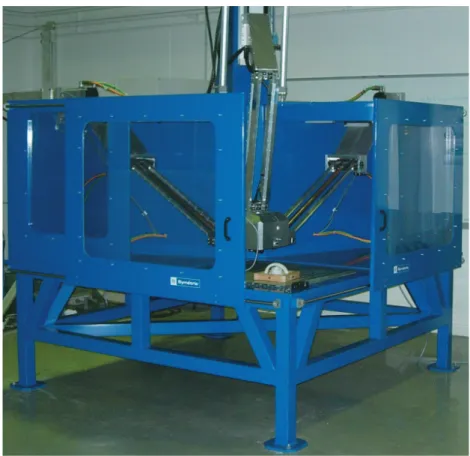
3.1 Prototype of the Orthoglide-5axis (IRCCyN) . . . 60

3.5 Orthoglide 5-axis cubic workspace . . . 63

3.6 Orientation of vector v (Traj I) . . . 64

3.7 Orientation of vector v (Traj II) . . . 65

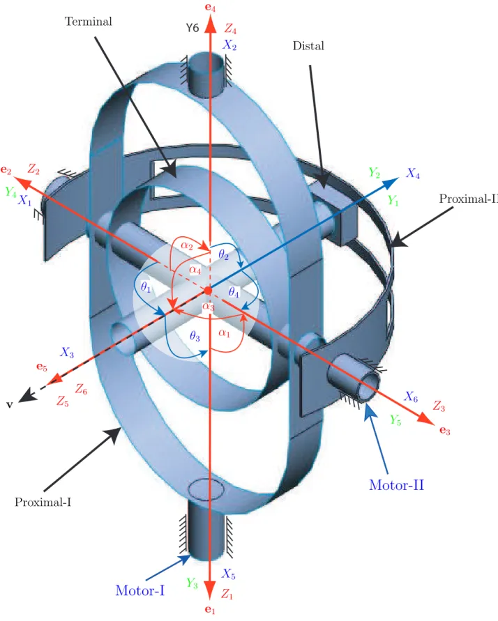
3.8 Definition of reference frames for Orthoglide Wrist . . . 69

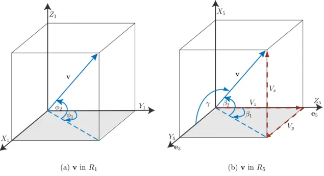
3.9 Definition of v in frames R1 and R5 . . . 72

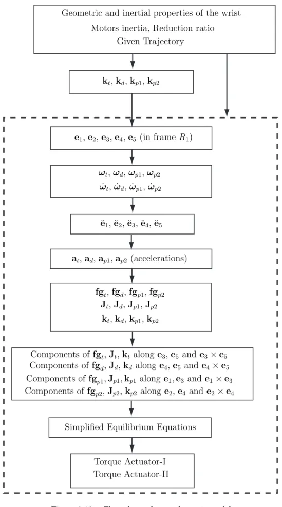
3.10 Flow chart of wrist dynamic model . . . 73

3.11 CAD model and FBD of terminal . . . 74

3.12 CAD model and FBD of Distal . . . 75

3.13 CAD model and FBD of Proximal-1. . . 77

3.14 CAD model and FBD of Proximal-2. . . 77

3.15 Compatibility Free body diagrams . . . 78

3.16 Orthoglide Wrist Parameters. . . 81

3.17 Wrist kinematics-Traj-I, R=0.200 m, φ = 90◦ . . . 83 3.18 Wrist kinematics-Traj-I, R=0.200 m, φ = 45◦ . . . 84 3.19 Wrist kinematics-Traj-II, R=0.200 m, γ = 45◦ . . . 85

3.20 Actuators torques vs time (Traj-I & II) . . . 85

3.21 Actuators maximum torques and powers vs R & γ . . . 86

3.22 Actuators torques for different values of γ . . . 87

3.23 Energy balance for wrist dynamics . . . 88

3.24 Terminal FBD with machining forces . . . 89

3.25 Actuators torques vs Time with machining forces . . . 90

3.26 Actuators maximum torques with machining forces . . . 91

3.27 Schematic of the Orthoglide 3-axis . . . 94

3.28 Simplified model of the Orthoglide 3-axis . . . 95

3.29 Prismatic joints position and rates for Traj-I (φ = 90◦ ) . . . 95

3.30 Prismatic joints position and rates for Traj-I (φ = 45◦ ) . . . 96

3.31 Prismatic joints position and rates for Traj-II (γ = 45◦ ) . . . 96

3.32 Orthoglide leg parameterization for the dynamic analysis . . . 97

3.33 Orthoglide 3-axis actuators forces for Traj-I and II (R=0.2 m) . . . 98

3.34 Max power requirement with four motors (Traj-II, η = 2) . . . 102

3.35 Max Power Requirement with four motors (Traj-II, η = 4/3) . . . 103

4.1 Path placement characterization . . . 111

4.2 Flowchart of mono-objective path placement optimization process . . . 118

4.3 Flowchart of multiobjective path placement optimization process . . . 121

4.4 Orthoglide 3-axis cubic workspace . . . 122

4.6 Orthoglide 3-axis ith _{leg . . . 124}

4.7 Test path characterization . . . 126

4.8 _{Test trajectory for a rectangular path of size 0.05 × 0.10 m}2 . . . 127

4.9 Cutting forces . . . 128

4.10 Locations of rectangular path with minimum energy consumption . . . 130

4.11 Locations of rectangular path with maximum energy consumption . . . 131

4.12 Emin and Emax and percentage saving for the rectangular test paths . . . . 131

4.13 Energy as a function of xOp and zOp for a 30 m×60 m rectangular path . . 132

4.14 Energy vs xOp and yOp for 30 m × 60 m rectangular path . . . 132

4.15 Energy as a function of xOp and yOp for different orientations (zOp = 0) . . 133

4.16 Energy as a function of xOp and φ for yOp = zOp = 0 . . . 133

4.17 Comparison of trajectory parameters for Emin and Emax locations . . . 134

4.18 modeFRONTIER model . . . 135

4.19 Pareto frontier for the Orthoglide 3-axis path placement . . . 137

4.20 Path locations for minimum and maximum objective functions . . . 138

4.21 Shaking forces experienced by three actuators for Emin and Iδf min . . . 139

1

List of Tables

1.1 General comparison of serial and parallel robots . . . 8

1.2 Classification of optimization problems . . . 22

2.1 Summary of performance measures . . . 35

2.2 Lower and upper bounds of the design variables . . . 52

2.3 modeFRONTIER algorithm parameters . . . 52

2.4 Three Pareto optimal solutions . . . 54

3.1 Orthoglide 5-axis workspace parameters . . . 63

3.3 DH-parameters for Orthoglide wrist . . . 70

3.4 Relations of θ1, θ2, θ3, θ4 . . . 71

3.5 Summary of θ1, θ2, θ3, θ4 relations . . . 71

3.6 Orthoglide wrist parameters . . . 82

3.7 Motors parameters of the Orthoglide Wrist . . . 83

3.8 Wrist kinematics and dynamics peak values for Traj.-II . . . 84

3.9 Maximum actuators torques and powers with machining forces . . . 92

3.10 Maximum prismatic joints rates and accelerations for test trajectories . . . 94

3.11 Parameters of the Orthoglide 5-axis arm . . . 98

3.12 Ball screw calculation for Orthoglide 5-axis . . . 99

3.13 Motors Parameters from Catalogue . . . 99

3.14 Preliminary Motors Tests. . . 100

3.15 Power requirements with different motors (η = 2) . . . 101

3.16 Power requirements for M3 and M4 motors (η = 4/3) . . . 102

3.17 Effect of the variation of wrist mass for M3 (η = 2) . . . 103

3.18 Effect of the variation of wrist mass for M4 (η = 2) . . . 104

4.1 Orthoglide 3-axis workspace parameters . . . 122

4.2 Orthoglide 3-axis actuators parameters . . . 122

4.3 Parameters of the Orthoglide 3-axis Leg . . . 124

4.4 Minimum and maximum energy used for a given rectangular path . . . 130

4.5 modeFRONTIER algorithm parameters . . . 135

1

Introduction

In the competitive world of today, the industries are overwhelmed with the high demand that the human being himself cannot achieve. It is is apparent that faster, more efficient, more productive and reliable systems are required. That is one of the reasons why more efficient robotic systems have to be developed.

Traditional robotic manipulators can be classified into two families: the serial and the pa-rallel manipulators. Serial manipulators are distinguished by the fact that they have only one independent kinematic chain between the base and the end-effector of the manipu-lator whereas the parallel manipumanipu-lators have more than one kinematic chains connecting the base and the end-effector.

Parallel manipulators, also known as Parallel Kinematics Machines (PKMs), have attrac-ted attention for their high speed, better accuracy, low mass/inertia properties and high structural stiffness. These are attractive features for the innovative machine-tool archi-tectures; however practical utilization for the potential benefits requires an extensive and efficient analysis of their structure, kinematics and dynamics.

PKMs design, like any other product design, goes through many phases and requires, as a prerequisite, a designer’s knowledge as well as years long experience for a design to be appreciable. A designer is faced with a great amount of variables and parameters, each one needed to be analyzed carefully. While some are more important than others, to know how important they are with respect to each other can be an exhaustive task. Still, there are times when less important variables play the most important role in the failure of an engineering structure. It is only natural that while dealing with a very complex design of enormous proportions, it is not possible for a designer to take into account all the variables simultaneously. An optimization process, however, does not require such an experience and it is faster than conventional design processes. Design optimization based on numerical algorithms and techniques can be applied to various engineering systems to help a designer come out with a proposal that is more efficient, light weight, reliable, safe, cost effective and that satisfies the user too. This requires not only the final product to

be optimized but also the optimization of manufacturing process as well as the optimum use/application of the product.

Conventional design techniques may be used for a trivial design of PKMs with a limited capability of considering the performance measures and constraints. However, for complex designs, with a large set of objectives and constraints, these techniques cannot adequately address the problem. A multiobjective optimization approach, on the other hand, can be used to identify a set of optimal trade-off solutions (called a Pareto set) between the conflicting design objectives/constrains, to gain a better understanding of the complexity of the PKMs design problem. Accordingly, in this thesis, some multiobjective optimization approaches are proposed for the design optimization of PKMs.

Research Directions and Contributions

– A multiobjective optimization approach to determine the optimal design parameters of a PKM is proposed in order to maximize its regular workspace and minimize the mass in motion. The performance of the mechanism within the workspace is guaranteed by constraining the condition number of the kinematic Jacobian matrix and stiffness characteristics.

– An approach to select proper actuators/motors is presented based on the kinematic and dynamic analysis of a parallel manipulator. Some test trajectories are proposed to analyze the mechanism and motors performance.

– A novel concept of single and multiobjective optimum path placement based on the electric energy consumption, shaking forces and actuators torque is introduced that deals with optimum use of a pre-designed in-use PKM.

Thesis Organization

This thesis report is composed of four chapters. The first chapter provides a state of the art of parallel manipulators and design optimizations. The other three chapters address three separate but inter-linked design optimization issues of PKMs.

The first issue addressed in the second chapter is that of dimensional synthesis of parallel manipulators. A multiobjective optimization problem is proposed to determine optimum structural and geometric parameters of parallel manipulators in order to minimize the mass of the components in motion and to maximize its workspace with desired manipu-lability and stiffness characteristics. The proposed approach is applied to the optimum design of a three-degree-of-freedom planar parallel manipulator.

The second topic addressed in the third chapter is the important issue of the actuators selection based on the dynamic model of the manipulators. The process focuses on the

3 kinematic and dynamic analysis of the Orthoglide 5-axis, a spatial PKM developed for high speed operations. The analysis is carried out firstly for the 2-dof spherical wrist of the Orthoglide 5-axis and then for the 3-dof translational parallel manipulator, the Orthoglide 3-axis. Some test trajectories are used to analyze the results and finally, a procedure of motors selection is proposed.

The fourth chapter deals with the optimal use of a PKM. Single and multi-objective path placement optimization approaches for PKMs are presented based on electric energy consumption, actuators torques and shaking forces. It proposes a methodology to deter-mine the optimal location of a given test path within the workspace of a PKM in order to minimize the electric energy used by the actuators, actuators maximal torques and the shaking forces subject to the geometric, kinematic and dynamic constraints. The proposed methodology is applied to the Orthoglide 3-axis, as an illustrative example.

1

Introduction to the

Parallel Robots and

Design Optimization

1.1 Introduction . . . 5

1.2 Parallel Robots . . . 6

1.2.1 Classification of Parallel Robots . . . 7

1.2.2 Planar Parallel Manipulators . . . 8

1.2.3 Spatial Parallel Manipulators . . . 9

1.2.4 Hybrid Manipulators . . . 10

1.2.5 Some Basic Parallel Architectures . . . 11

1.3 Design Aspects of Parallel Robots . . . 13

1.3.1 Kinematics . . . 14

1.3.2 Dynamics . . . 16

1.3.3 Singularities. . . 16

1.4 Design Optimization . . . 17

1.4.1 Optimization Process . . . 19

1.4.2 Classification of Optimization Process . . . 20

1.4.3 Multiobjective Optimization and Pareto Optimality . . . 20

1.5 Conclusion . . . 23

This chapter presents a brief overview of the parallel kinematic machines or parallel robots. It covers general introduction, some of the design aspects and performance measures of the parallel manipulators. Some typical parallel architectures are also presented. At the end, an introduction to the optimization process addressing single and multiobjective optimizations formulations is presented.

1.1

Introduction

Parallel mechanisms have attracted attention for high speed and accuracy applications due to their conceptual potentials in high motion dynamics and accuracy combined with low mass/inertia properties, high structural stiffness (i.e. stiffness-to-mass ratio) due to their closed kinematic loops (Brog˚ardh, 2007; Weck and Staimer, 2002; Chanal et al., 2006;

manipulators that have already reached the dynamic performance limits (Pashkevich et al.,

2009b). These features are induced by their specific kinematic structure, which resists to the error accumulation in kinematic chains and allows convenient actuator location close to the manipulator base. Besides, the links work in parallel against the external force/torque, eliminating the cantilever-type loading and increasing the manipulator stiff-ness (Pashkevich et al.,2009b;Tsai,1999). Parallel robots are attractive for the innovative machine-tool architectures (Tlusty et al., 1999; Wenger et al., 1999), but practical utili-zation for the potential benefits requires development of efficient kinematic and dynamic analysis, which satisfy the computational speed and accuracy requirements of relevant design procedures (Pashkevich et al.,2009b).

1.2

Parallel Robots

Traditional robotic manipulators can be classified in two families: the serial and the pa-rallel manipulators. Serial manipulators are distinguished by the fact that they have only one independent kinematic chain between the base and the end-effector of the manipu-lator. These are opened-loop mechanisms, namely, composed of an open kinematic chain with each intermediate link coupled with two other links by means of two actuated joints. One end of this chain is fixed to the base while the other end is the end-effector. The presence of single kinematic chain and the absence of any passive joint make the serial manipulators simpler to design and to analyze.

Figure 1.1 – Schematic of a serial robot

On the contrary, the parallel manipulators have several legs connecting the base and the end-effector (EE), also called moving platform (MP). Each leg is a kinematic chain whose end links are connected to the two platforms, i.e. base and end-effector. Contrary to serial manipulators, where all joints are actuated, parallel manipulators also contain passive joints. The inclusion of passive joints causes their analysis more complex than the

1.2 Parallel Robots 7

Figure 1.2 – Schematic of a Parallel robot

analysis of their serial counterparts. Parallel manipulators are closed-loop mechanisms presenting very good performance in terms of accuracy, velocity, stiffness and ability to manipulate large loads. They have already been used for many applications like machi-ning (Bruzzone et al., 2002), medical robotics (Pisla et al., 2008), space (Rojeski, 1972;

Thompson and Campbell, 1997), astronomy (Su et al., 2003), flight-simulators (Baret,

1978) for the design of earthquake simulators (French et al., 2004).

Serial manipulators are more common in industry due to their simple kinematics and ac-cessibility of well developed and matured technical design and analysis material. Another advantage of serial manipulators is the availability of large workspace compared to their own size. However serial manipulators have many limitations some of which include low stiffness, low payload, low accuracy, high inertia etc. Major drawbacks of parallel mani-pulators are their limited workspace and difficult kinematic analysis. A summary of the comparison of the general features of serial and parallel manipulators presented in (Kuen,

2002) is given in Table 1.1.

1.2.1

Classification of Parallel Robots

The parallel robots can be compared based on several criteria. For instance,(Company,

2006) used the following criteria to compare some parallel robots: – Mechanism number of degrees of freedom (dof)

– Type of dof

– Mechanism features (constant legs length, variable legs length,...) – Mechanism dimensions (as for Gough-like platforms)

Table 1.1 – General comparison of serial and parallel robots (Kuen,2002)

Feature Serial Robots Parallel Robots

Workspace large small

Stiffness low high

Singularity Problems some abundant

Payload low high

Inertia large small

Structure simple complex

Accuracy error accumulated error average out

Speed low high

Acceleration low high

Forward Kinematics simple complex

Inverse Kinematics complex usually simple

Dynamics relatively simple complex

Design Complexity low high

– Actuators placement and number regarding mechanism dof

– Number of kinematic chains (fully parallel, kinematics redundancy, actuation re-dundancy, hybrid mechanisms...)

A detailed survey of the different classifications of parallel manipulators can be found in (Company, 2000)

1.2.2

Planar Parallel Manipulators

As their name indicates, planar parallel manipulators (PPMs) generate planar motions. Usually, their kinematics and control are simple. A Two-dof and a three-dof PPMs are shown in Figs. 1.3 and 1.4, respectively.

ρ1 ρ2

P (x, y)

X Y

1.2 Parallel Robots 9 PPM can find their uses in stand alone applications, particularly, when planar motions are required with high speed and precision, like laser or water jet cutting and pick-and-place operations. They can also be used as simple sub-elements in more complex mechanisms (Company,2006). Some machining applications with such devices are given in (Katz et al.,

2001). ρ1 ρ2 ρ3 θ P (x, y) X Y

Figure 1.4 – A 3-dof planar parallel manipulator

1.2.3

Spatial Parallel Manipulators

Spatial parallel manipulators (SPMs) can have more than 3-dof and have the ability to move in the three dimensional space. These manipulators have various architectures and can be used in a vast milieu of robotic applications. We can find a great amount of SPMs in the literature (Stewart, 1965; Clavel, 1988; Kong and Gosselin, 2002, 2004;

Liu et al., 2005; Gogu, 2006). Some of the famous architectures of spatial robots are Delta architecture (Clavel, 1988), Star architecture (Herv´e and Sparacino, 1992), Tsai architecture (Tsai, 1996) and Stewart platform (Stewart, 1965). Star and 3-UPU Tsai architectures are shown in Figs.1.5and1.6, respectively, whereas Delta robot and Stewart platform are briefly presented in the coming sections.

Figure 1.5 – Star Architecture (Herv´e and Sparacino, 1992)

Fixed Base

Moving Platform

Figure 1.6 – 3-UPU Tsai Architecture (Tsai, 1996)

1.2.4

Hybrid Manipulators

Hybrid manipulators are usually a concatenation of serial and parallel architectures where only a part of the mechanism is based on parallel kinematics. According to Krut (2003),

1.2 Parallel Robots 11 a mechanism is hybrid if it has several kinematic chains between the base and the plat-form with at least one of them including more than one actuator. For example, parallel manipulators with a serial wrist and serial manipulators with a parallel wrist can be clas-sified as hybrid manipulators. These hybrid manipulators can gather the advantages of both serial and parallel manipulators. For example a hybrid manipulator can have large workspace thanks to the serial architecture and a good accuracy and stiffness thanks to the parallel chain. Figure 1.7 depicts a concatenation of a Delta type manipulator and 3-UPS platform, namely, a hybrid manipulator (Gallardo-Alvarado, 2005).

Fixed Platform

Translational Platform End-Platform

Independent Limb

Passive Kinematic Chain O

X

Y Z

Figure 1.7 – Hybrid robot (Gallardo-Alvarado, 2005)

1.2.5

Some Basic Parallel Architectures

The Delta manipulator, designed by Clavel (1988), is a well known 3-dof translational parallel manipulator. It is composed of three identical limbs connecting the moving plat-form to the base as illustrated in Fig. 1.8. Each limb contains a revolute joint and a parallelogram joint and another revolute joint.

Figure 1.8 – Basic Delta architecture

kinematics chains of type R − R − Pa− R where R and Pa stand for revolute and paral-lelogram joints respectively. These paralparal-lelograms constrain some rotation of the moving platform and enable it to move in pure translation along X, Y and Z directions. Actuators are fixed and are located at the base of the robot. Actuators can be of linear or of rota-tional type. Three kinematic chains connect the base with the platform or end-effector. An additional actuator and a central telescopic bar can be added to provide a rotational degree of freedom about the axis of symmetry of the robot, hence yielding a four-dof robot. This is the case of commercially available Delta robot devoted to pick and place operation like the Flexpicker robot from ABB shown in Fig. 1.9.

As the actuators are located at the base and the moving parts are light, Delta robots have small inertia hence have good dynamic performance. As a matter of fact, they can achieve a velocity equal to 10m/s and accelerations up to 20g (Krut, 2003). Due to high speed of the Delta robot, it is widely used in packaging, medical, pharmaceutical and electronic industry.

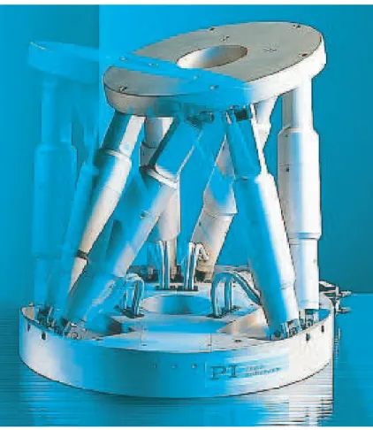
1.2.5.2 Stewart Platform

Stewart platform, also known as Gough-Stewart platform or Hexapod,is a PKM having six degrees of freedoms, developed by Gough and Whitehall (1962) and Stewart (1965). The mechanism consists of a stationary base platform and a mobile platform connected with each other with six kinematics chains or legs. The legs have actuated prismatic joints allowing the change of the length of each leg. The legs are connected to the base and the

1.3 Design Aspects of Parallel Robots 13

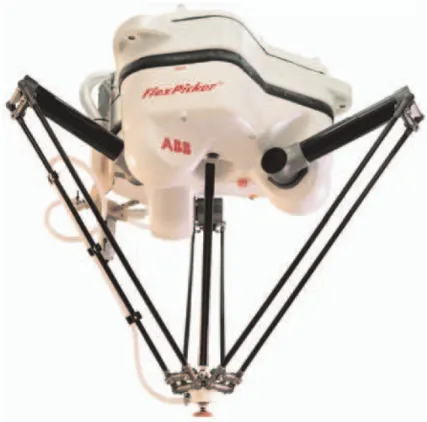
Figure 1.9 – FlexPicker (ABB)–Delta Robot

mobile platform by means of universal joints, (Figs. 1.10 and 1.11).

The desired position and orientation of the mobile platform can be achieved by varying the lengths of the six legs, i.e., transforming six translational motions of prismatic joints into three positional (x, y, z) and three rotational (pitch, yaw, roll) degrees of freedom of the mobile platform.

Stewart platform or its counterparts (Hexapods etc) are widespread in the literature. The Stewart platforms are mainly used in the design of flight simulators, for virtual reality, machine tool technology, crane technology, satellite dish positioning, telescopes and medical applications.

1.3

Design Aspects of Parallel Robots

Parallel robots offer promising advantages over their serial counterparts like high stiffness, high accuracy, high dynamic capacity, low inertia and a better payload-to-weight ratio (Merlet, 2006c; Tlusty et al., 1999; Wenger et al., 1999; Majou et al., 2001). However, the closed-loop nature of the mechanism leads to complex kinematics, difficult trajectory planning, small and complicated workspace with singularities and non linear input/output relations (Angeles, 2002).

Platform

Base

Figure 1.10 – General Stewart Platform Structure

1.3.1

Kinematics

Robot kinematics is the study of the relationship between the joint parameters and the corresponding pose of the end-effector. Inverse kinematic model (IKM) determines the required joint parameters for a given end-effector pose whereas direct or forward kinematic model (DKM) determines the end-effector pose for a known set of joint coordinates. The IKM is expressed as follows:

xp = f (q) (1.1)

and the DKM as: q = f−1

(xp) (1.2)

where q is the vector of active joints variables and xp is the vector of operational coordi-nates of the end-effector.

Similarly, direct velocity model (DVM) defines the Cartesian velocities of the end-effector in terms of joint rates, i.e.,

1.3 Design Aspects of Parallel Robots 15

Figure 1.11 – Stewart Platform

And, inverse velocity model (IVM) determines joint rates as a function of the Cartesian velocities of the end-effector, i.e.,

˙q = J−1p ˙xp (1.4)

where, Jp is the robot Jacobian matrix, ˙xp is the end-effector velocity vector comprising of linear and angular velocity components and ˙q is the actuated joints velocity vector. Eq. (1.3) can also be written as:

A ˙xp = B ˙q (1.5)

where A and B are the parallel and serial Jacobian matrices (Gosselin, 1990b). As long as matrix A is not singular, we have, Jp = A−1B.

Finally, the second order velocity model (or acceleration model) expresses the accelera-tion of the end-effector in terms of the acceleraaccelera-tions and velocities of the actuated joints variables which can be derived upon differentiation of Eq. (1.3):

¨

The kinematics of parallel robots along with various practical examples and applications have been thoroughly presented by Merlet (2006c) and Angeles (2002). Besides, we can find the kinematic model of a general Stewart-Gough platforms in (Husty, 1996), the kinematic analysis of the Delta robot in (Clavel, 1988) and the one of the Orthoglide, a 3-dof translational PKM, in (Wenger and Chablat, 2000). A state of the art of the kinematics of the PKMs is given by Zentner (2005),Nielsen (1999) and Erdman(1993).

1.3.2

Dynamics

Forces and torques acting on the robot are related to the resulting robot motion by its dynamics. Robot dynamics deals with the determination of the relations between joint forces and the generalized accelerations, velocities and coordinates of the end-effector. The Inverse Dynamic Model (IDM) gives the relation between the actuated joint forces/torques for a given trajectory, velocities and acceleration of the end-effector whereas the Direct Dynamic Model (DDM) gives the relation between the end-effector trajectory, velocities and acceleration for a known or given actuated joints forces/torques. The knowledge of robots dynamics is of prime importance to understand the robot performance and for the command and control. Particularly, dynamics plays an important role in the control of PKMs, high bandwidth robots and structurally sensitive robots (Merlet, 2006c).

The dynamics of PKMs has been an area of interest of several researchers (Fichter, 1986;

Lee and Shah, 1988; Sugimoto, 1989; Reboulet and Berthomieu, 1991; Sklar and Tesar,

1998). To develop the dynamic model of parallel robots, several approaches have been pro-posed, including the Newton-Euler formulation (Sugimoto,1989;Dasgupta and Choudhury,

1999), Lagrange approach (Miller and Clavel,1992), principle of virtual work (Tsai,2000), screw theory (Gallardo-Alvarado et al.,2003) or principle of Hamilton (Miller,2004). An introduction to different approaches to derive the IDM and DDM of PKMs can be found in (Merlet,2006c; Angeles, 2002; Ibrahim, 2006).

1.3.3

Singularities

Singularities is one of the major issues of parallel robots and has been a prime focus of research of several roboticians. At singular configurations, robots are exposed to unusual behaviors as loss or gain of degrees of freedom, unattainable directions of motion, exis-tence of motion while the actuators are locked (Pashkevich et al.,2009b).Merlet (2006c) defines the singular configurations as the particular poses of the end-effector, for which parallel robots lose their inherent infinite rigidity, and in which the end-effector will have uncontrollable degrees of freedom.

One of the earlier singularity analysis of a closed-loop kinematic chain is that of Hunt

(1978). Other pioneers to define and study singularities of closed-loop kinematic chains are Gosselin(1990b);Gosselin and Sefrioui(1991);Merlet (2006c,1989);Ma and Angeles

1.4 Design Optimization 17 (1991a);Zlatanov et al.(1994,1995);Mohammadi Daniali et al.(1995) andPark and Kim

(1999).

In general kinematic singularities of mechanisms can be classified into six different classes (Zlatanov et al.,1994), whereas there are two basic types of singularities (Gosselin,1990b), namely, parallel and serial singularities.

A parallel singularity occurs when the determinant of the parallel Jacobian matrix, A, vanishes, i.e. |A = 0| (Gosselin,1990b). At this configuration, end-effector can move with locked actuated joints, which results in an absence of control of the end-effector or tool-point P . Figure 1.12 shows a parallel singular configuration of 2-dof mechanism, Biglide. These singularities can damage the mechanism and have to be eliminated from the works-pace (Majou and Chablat, 2007).

P

Figure 1.12 – Biglide-parallel singular configuration

A serial singularity occurs when the determinant of the serial Jacobian matrix, B, va-nishes, i.e. |B = 0| (Gosselin,1990b). This type of singularity results in a loss of degree of freedom of the mechanism, i.e. at this configuration, there exists a direction along which no motion can be produced. Figure 1.13represents the serial singular configuration of the Biglide. Serial singularities define the boundary of the Cartesian workspace of the parallel kinematic machines (Merlet, 2006c).

P

Figure 1.13 – Biglide-serial singular configuration

1.4

Design Optimization

Humans have been exploiting and manipulating their knowledge, experience and resources since pre-historic times to maker their living better and easier. In other words they have

been optimizing their resources for better yields. In simple words, optimization is a process of increasing the overall output while reducing the input at the same time. Development of industrial tyres is just one good example to realize the humans’ desire to improve their usage of resources, from a very inefficient triangular to very efficient circular one, it has gone through many phases gradually reducing the effort and hence increasing the mechanical efficiency. In order to increase the strength to weight ratio, the use of hollow cylindrical shafts compared to solid ones is another good example.

Off course, optimization is not just limited to tyres or shafts; it now encompasses whole range of engineering applications in every field of endeavour. From automobiles to aircrafts and satellites, watercrafts to trains, housing projects to giant bridges, simple objects like needles to state of the art robots, and from civil to military applications, optimization has been a key area of interest in all applied fields.

Humans are consuming the resources made available to them by the nature in growing numbers. To say the obvious; not all of these resources are renewable, it is therefore increa-singly important, logically and environmentally, to optimize our use of these resources. Optimization may therefore be rightly said as one of the most crucial tools in humans’ battle for survival.

Engineering design process goes through many phases and requires, as a prerequisite, a designer’s knowledge as well as years long experience for a design to be appreciable. A de-signer is confronted with myriad variables and parameters, each seeking careful attention and indulgence. While some are more important than others, the very designation of the level of importance can itself be an exhaustive task. Still, there are times when ”less im-portant” variables play the most important role in the failure of an engineering structure. It is only natural that while dealing with a very complex design of enormous proportions, it is not possible for a designer to take into account all the variables simultaneously. An optimization process, however, does not demand this much experience and yet it is faster than a conventional design process. Design optimization based on numerical algorithms and techniques can be applied to varied engineering systems to help a designer come out with a proposal that is more efficient, light weight, reliable, safe, cost effective and that satisfies the end user too. This requires not only the final product to be optimized but also the optimization of manufacturing process as well as the tools to manufacture those products at every level of production. A lot of research has been done in the field of op-timization, proposing different approaches, techniques and methodologies. They span a large range of problems such as linear programming, constrained/unconstrained non-linear optimization, single and multi-objective optimization.

1.4 Design Optimization 19

1.4.1

Optimization Process

Optimization process in design is a tool of conceptualization and analysis used to achieve better designs or design improvements. It is a mathematical procedure for determining optimal solutions by representing all the complexities of the design in the form of de-sign variable(s), objectives function(s) and/or constraint(s). The basic elements of any constrained optimization problem are:

Objective function. An objective function or vector of objective functions is the mathematical expression that expresses the optimization goal in terms of design variables. Optimization process is required to either minimize or maximize the ob-jective function. For instance, in robotics, maximization of the workspace or mini-mization of inertia/mass of a manipulator can be the objective functions.

Design variables. Also known as decision variables, are the “unknowns” of the opti-mization problem which are to be determined. From the point of view of the designer, these are the controllable numeric values which affect the value of the objective func-tion. Design variables can be continuous (such as a length/diameter/cross-section of the robot links) or discrete (such as the number of links/joints in a robot). Constraints. A set of constraints that must be satisfied in order for the design to be feasible. These are mathematical expressions that combine the variables to express limits on the possible solutions. Constraints allow the design variables to take certain values but exclude others. In addition to physical laws; constraints can reflect resource limitations, user requirements, or bounds on the validity of the analysis models.

Variable bounds. Design variables are not usually permitted to take any value. Instead, these are usually have lower and upper limits, known as variable bounds. Variable bounds limits the design space and along with constraints, used to distin-guish the solutions as feasible or unfeasible.

The optimization problem is then:

Find the values of the design variables that minimize or maximize the objective function while satisfying the constraints. Remembering that variables describe all situations and constraints describe all feasible situations Mathematically, an single-objective optimiza-tion problem can be expressed as:

min x f subject to:      gi(x) 6 0 i = 1, · · · m hj(x) = 0 j = 1, · · · n xl 6x 6 xu (1.7)

Where, x is the vector of design variables, f is the objective function to be minimized subject to m inequality and n equality constraints given by gi(x) and hj(x), respectively.

Optimization is an iterative process and involves at least some degree of trial and errors. As the problem complexity is increased, the search procedure becomes tedious and may not guarantee a solution in all cases. The main steps involved in solving an optimization problem can be cited as (Arora, 1989):

– understand the problem, by drawing a diagram or flow chart which represents the problem;

– write a problem formulation in words, including decision variables, objective func-tion, and constraints;

– write the algebraic formulation of the problem; o define the decision variables;

o write the objective function(s); o write the constraints;

develop a spreadsheet model;

– set up the Solver settings and solve the problem;

– examine the results and make corrections to the model; – analyze and interpret the results.

The overall structure of an optimization approach is presented in Fig. 1.14.

1.4.2

Classification of Optimization Process

There are many optimization algorithms available to solve an optimization problem. Many methods are appropriate only for certain types of problems. Thus, it is important to be able to recognize the characteristics of a problem in order to identify an appropriate method to solve the problem. Within each class of problems there are different minimization methods, varying in computational requirements, convergence properties, and so on. Optimization problems are classified according to the mathematical characteristics of the objective function, the constraints, and the control variables. Other classifications are summarized in Table1.2. Normally, optimization problems found in engineering are the combinations of different classifications. For instance, a problem may be of the type “constrained nonlinear multiobjective optimization”

1.4.3

Multiobjective Optimization and Pareto Optimality

In numerous real life optimization applications, there exist many targets or objectives that should be optimized simultaneously. However, these targets often conflict and it is not possible to satisfy all of them at the same time. Thus one has to make compromises. Such types of optimization problems are called multiobjective optimization problems.

1.4 Design Optimization 21

Identify i. Design variables ii. Objective function iii. Constraints

Collect data to describe the system

Estimate initial design

Analyze the system

Check the constraints

Does the design satisfy the convergence criterion(a)?

Update the design using an optimization scheme

Yes

No

Stop

Figure 1.14 – General design optimization process (Arora, 1989)

A general multiobjective optimization problem is to find design variables that optimize a vector objective function subject to a number of constraints and bounds. It is often formalized as follows (Shan and Wang, 2005):

min x F (x) = (f1(x), . . . ,fm(x), . . . fk(x)) (1.8) subject to: gk(x) 6 0 k = 1, · · · p hj(x) = 0 j = 1, · · · q xl r 6xr 6xur r = 1, · · · n

where the components of the multiobjective function F (x), are usually in conflict with one another with respect to their own optimum point. The design variable vector, x = [x1, · · · xr, · · · ,xn], consists of n design variables of the problem bounded by xl and xu. hj(x) and gk(x) are equality and inequality constraints, respectively.

Table 1.2 – Classification of optimization problems (Jilla, 2002)

Characteristic Property Classification

Number of Control variables

One Single variable

More than one Multivariable

Type of control variables

Continuous real number Continuous

Integers Discrete

Continuous real number and integers Mixed Integer Problem functions

Linear function of control variables Linear Quadratic functions of the control variables Quadratic nonlinear functions of the control variables Nonlinear Problem formulation Subject to constraints Constrained

Not subject to constraints Unconstrained Number of Objective

function

One Mono objective

More than one Multiobjective

Contrary to the traditional mono-objective optimization, multiobjective optimization pro-blems have several objective functions to optimize at the same time. In addition, there is not a unique solution, but instead there can be a number of mathematically equivalent good solutions. Best solution means a solution not worst with respect to any of the ob-jectives and at least better in one objective than the other. An optimal solution is the solution that is not dominated by any other solution in the search space. Such an optimal solution is called Pareto optimal and the entire set of such optimal trade-offs solutions is called Pareto optimal set (Abraham et al., 2005).

f1 f2 A B C Feasible Space Pareto Frontier

1.5 Conclusion 23 Pareto optimal can be defined as (Marler and Arora,2004), A point x∗

∈ X is Pareto

op-timal if and only if there does not exist another point x ∈ X, such that fi(x) 6 fi(x∗) and

fi(x) < fi(x∗) for at least one function. Pareto optimal points are also known as efficient, non-dominated, or non-inferior points. Even though there are several ways to approach a multiobjective optimization problem, most work is concentrated on the approximation of the Pareto set (Abraham et al., 2005). Determination of some Pareto subsets, where the solution or its part must lie, decreases the design space which results a reduction of the overall computational complexity of the design task. The storage of any design va-riant, computed intermediately, can be used for numerical determination of the Pareto set (Valasek and Sika,2003;Caro et al., 2007; Bouyer et al., 2007).

There are several approaches to solve multiobjective optimization problems. Some examples of these approaches are weighted sum method, weighted product method, weighted min-max method, exponential weighted criterion, Lexicographic method, goal programming methods, physical programming, genetic algorithms and simulated annealing. A survey of these and others multiobjective optimization approaches can be found in (Marler and Arora,

2004; Andersson,2001).

1.5

Conclusion

The parallel kinematics machines are getting more and more attention in modern indus-trial applications for their potential benefits of high speed, good accuracy, low mass/inertia properties and high structural stiffness. However, practical utilization for these added be-nefits requires an extensive and efficient analysis of their structure, kinematics and dyna-mics. On the design front, use of optimization techniques is a prime area of interests of the researchers in order to optimize the existing designs or to explore new design prospects. The use of computer aided design (CAD), computational fluid dynamic (CFD) and finite element methods (FEM) has reduced the time-consuming design and analysis process with better results. Conventional design techniques may be used for a trivial design of PKMs with a limited capability of considering the performance measures and constraints. Nu-merical optimization techniques, on the other hand, can be very useful to obtain solution variants, i.e., set of reliable and acceptable solutions obtained by following a systematic approach instead of hit and trail or heuristics approaches.

In the next chapter, various performance measures of PKMs will be discussed and sub-sequently a multiobjective optimization approach will be presented in order to determine optimum design parameters of a PKM.

2

Multiobjective Design

Optimization of Parallel

Kinematics Machines

2.1 Introduction . . . 26

2.2 Performance Measures and Indices . . . 28

2.2.1 Workspace . . . 28

2.2.2 Manipulability . . . 29

2.2.3 Condition Number of the Kinematic Jacobian Matrix . . . 30

2.2.4 Accuracy . . . 31

2.2.5 Robustness and Sensitivity . . . 32

2.2.6 Stiffness . . . 32

2.2.7 First Natural Frequency . . . 34

2.2.8 Summary of Performance Measures and Indices . . . 35

2.3 Case Study: 3–PRR Manipulator . . . 36

2.3.1 Architecture of 3-PRR . . . 37

2.3.2 Inverse and Direct Kinematic Model of 3-PRR . . . 37

2.3.3 Jacobian Matrices of 3–PRR . . . 38

2.3.4 Dexterity of 3-PRR . . . 41

2.3.5 Stiffness Matrix. . . 41

2.4 Multiobjective Design Optimization of PKMs Problem Formulation 45

2.4.1 Optimization objectives . . . 45

2.4.2 Optimization Constraints . . . 46

2.4.3 Problem Statement. . . 47

2.5 Multiobjective Optimization Problem Formulation for 3–PRR 47

2.5.1 Optimization Design Parameters . . . 48

2.5.2 Optimization objectives . . . 48

2.5.3 Optimization constraints. . . 49

2.5.4 Problem Statement for 3–PRR . . . 51

2.5.5 Optimization Results. . . 51

2.6 Conclusion . . . 55

This chapter addresses the dimensional synthesis of parallel kinematics machines. A mul-tiobjective optimization problem is proposed in order to determine optimum structural and geometric parameters of a parallel manipulator. The proposed approach is applied to the optimum design of a three-degree-of-freedom planar parallel manipulator in order

to minimize the mass of the mechanism in motion and to maximize its regular shaped workspace.

2.1

Introduction

The design of parallel kinematics machines is a complex subject. The fundamental pro-blem is that their performance heavily depends on their geometry (Hay and Snyman,

2004) and the mutual dependency of almost all the performance measures. This results computational complexity of the problem and makes the traditional solution approaches inefficient. As reported by Merlet (2006c), since the performance of parallel manipulators depends on their dimensions, customization of these manipulators for each application is absolutely necessary. Furthermore, numerous design aspects contribute to the PKM performance and an efficient design will be that which takes into account all or more of these design aspects. For instance, a simplified design network of a parallel kinematics machine is shown in Fig.2.1 (Valasek et al.,2005). In this figure, eight design criteria are considered, namely, workspace, collision avoidance, dexterity and force transmission eva-luation, stiffness and eigen-frequency (modal) evaeva-luation, dynamic capability evaeva-luation, kinematic and elastostatic accuracy evaluation and finally control system dynamics and accuracy evaluation. The design process has been decomposed into three levels of design conflicts and related structural and parametric optimizations (Valasek et al.,2005):

Kinematics Dimensions Dimensions Cross-section Material Control Parameters

Max Max Max Max Max Max Max Min Max/Min

Workspace Workspace Workspace CollisionsCollisionsCollisions

Dexterity Dexterity Dexterity Force Transfer Force Transfer Force Transfer Stiffness Stiffness

Stiffness CapabilityCapabilityCapabilityDynamicDynamicDynamic

Eigenfrequencies Eigenfrequencies Eigenfrequencies Vibration modes Vibration modes Vibration modes Elastostatic Elastostatic Elastostatic accuracy accuracy accuracy Calibration Calibration

Calibration DynamicsDynamicsDynamicsControlControlControl AccuracyAccuracyControlControlControl Accuracy

Accuracy Accuracy

Accuracy

Geometry Embodiment design _Actuator

Geometrical design iterations

Structural design iterations

Actuator design iterations

2.1 Introduction 27 – geometric design conflicts: workspace, collision versus necessary dimensions for

stiff-ness, accuracy, dexterity and other requirements.

– structural design conflicts: stiffness, accuracy, eigen-frequencies versus mass, dyna-mics, acceleration etc;

– actuator design conflicts: drive torque versus drive inertia, the influence of control system.

From this general description of a PKM design process, it is obvious that it is an itera-tive process and an efficient design requires a lot of computational effort and capability for mapping design parameters into design criteria (objectives, constraints) and hence following a multiobjective design procedure. The design parameters of a PKM can be determined by using multiobjective optimization techniques where the design variants can be obtained from the generated Pareto frontiers. Modern optimization techniques can serve the purpose of this customization process and can facilitate the designer to come up with more efficient and cost-effective solutions. Therefore, design optimization of parallel mechanisms has become a key issue for their development and has gained more and more attention of the researchers in the recent years. Several researchers have addressed the optimization problem of parallel mechanisms to optimize their performance with respect to a single or several design objectives.

Lou et al. (2005, 2008) presented a general approach for the optimal design of paral-lel manipulators to maximize the volume of an effective regular-shaped workspace while subject to dexterity constraints. Effective regular workspace reflects simultaneously the requirements on the workspace shape and quality. Hay and Snyman (2004) considered the optimal design of parallel manipulators to obtain a prescribed workspace whereas

Ottaviano and Ceccarelli (2001) proposed a formulation for the optimum design of 3-dof spatial parallel manipulator architectures for given position and orientation workspaces.

Hao and Merlet (2005) discussed a multi-criteria optimal design methodology based on interval analysis to determine the possible geometries satisfying two compulsory require-ments of the workspace and accuracy. Ottaviano and Ceccarelli (2000) based their study on the static analysis and the singularity loci of a manipulator in order to optimize the geometric design of the Tsai manipulator for a given free from singularity workspace. Similarly,Ceccarelli et al.(2005) dealt with the multi criteria optimum design of both pa-rallel and serial manipulators with the focus on the aspects of workspace, singularity, and stiffness. Gosselin and Angeles (1988, 1989) studied the design of a planar and a 3-dof spherical parallel manipulators by maximizing the workspace volume while taking into account the condition numbers of these manipulators. Pham and Chen (2003) suggested maximizing the workspace of a parallel flexure mechanism with the constraints on a global and uniformity measure of manipulability.Stamper et al.(1997) used the global condition index based on the integral of the inverse condition number of the kinematic Jacobian

matrix over the workspace, to optimize a spatial 3-dof translational parallel manipulator.

Stock and Miller (2003) formulated a weighted sum multi-criteria optimization problem with manipulability and workspace as two objective functions. Menon et al. (2009) used the maximization of the first natural frequency as an objective function for the geometri-cal optimization of the parallel mechanisms. Similarly,Li et al.(2009) proposed dynamics and elastodynamics optimization of a 2-dof planar parallel robot to improve the dynamic accuracy of the mechanism. They proposed a dynamic index to identify the range of na-tural frequency with different configurations.Krefft and Hesselbach (2005) also presented multi-criteria elastodynamic optimization of parallel mechanisms while considering works-pace, velocity transmission, inertia, stiffness and first natural frequency as optimization objectives.Chablat and Wenger (2003) proposed an analytical approach for the architec-tural optimization of a 3-dof translational parallel mechanism, Orthoglide 3-axis, based on prescribed kinetostatic performance in a given Cartesian workspace.

In this chapter, we propose a methodology to deal with the multiobjective design optimi-zation of PKMs. The mechanism mass, conditioning number of the kinematic Jacobian matrix and accuracy characteristics are considered as objective functions. The propo-sed approach is highlighted by means of a 3-dof planar parallel manipulator and Pareto frontiers are obtained using a multiobjective genetic algorithm.

2.2

Performance Measures and Indices

The estimation of the manipulators performance is very important for proper manipula-tors application, design and selection. Angeles (2002) defines a performance index of a robotic mechanical system as a scalar quantity that measures how well the system be-haves with regard to force and motion transmission. Different authors have proposed va-rious performance characteristics and indices to compare and evaluate manipulators’ per-formance. Workspace (Wenger and Chablat, 2000; Liu et al., 2004; Stamper et al., 1997;

Kosinska et al.,2003), dexterity (Merlet,2006c), manipulability (Yoshikawa,1985;Merlet,

2006b;Kucuka and Bingulb,2006), accuracy (Merlet,2006b), stiffness (Pashkevich et al.,

2009b) are widely used performance characteristics of robot manipulators.

2.2.1

Workspace

Workspace is one of the most important issues as it defines the working volume of the robot/manipulator and determines the area that can be reached by a reference frame located on the moving platform or end-effector (Liu et al., 2004; Stamper et al., 1997;

Kosinska et al.,2003). The size and shape of the workspace are of primary importance for the global geometric performance evaluations of the manipulators (Wenger and Chablat,

2.2 Performance Measures and Indices 29 constant orientation workspace, maximal or reachable workspace, inclusive orientation workspace, total orientation workspace and finally the dextrous workspace. The constant orientation workspace is the region which can be reached by the end-effector with constant orientation. The region which can be reached by the end-effector with at least one orien-tation is the maximal or reachable workspace. The inclusive workspace is the region that can be attained by the end-effector with at least one orientation in a given range. Total orientation workspace defines the region which can be reached by the end-effector with every orientation of the end-effector in a given range and finally the dextrous workspace describes the region that can be reached by the end-effector with any orientation of the end-effector. Chablat et al. (2004) introduced the concept of regular dextrous workspace, which is defined as regular-shaped workspace within the Cartesian workspace in which the velocity amplification factors remain within a predefined range. This ensure good and homogeneous kinematic performance throughout the dextrous workspace.

In the literature, different methods to determine workspace of parallel manipulators have been proposed (Gosselin, 1990b; Merlet and Mouly, 1998; Merlet, 1995). These include, analytical methods (Kohli and Spanos,1985;Abdel-Malek and Yeh,1997), numerical, ite-rative and statistical methods mainly based on the discretization of the pose parame-ters (Lee and Yang,1983;Rastegar,1990;Alciatore and Ng,1994;Cleary and Arai,1991;

Ferraresi et al.,1995;Kumar and Waldron,1981), optimization methods (Lee and Cwiakala,

1985) etc. Some of the research works on the workspace analysis can be reported as (Merlet, 2006c; Gosselin, 1990b; Merlet and Mouly, 1998; Chablat et al., 2004; Gosselin,

1990a; Tsai and Soni, 1981; Gupta and Roth,1982).

2.2.2

Manipulability

The concept of manipulability of a manipulator was introduced by Yoshikawa (1985). The manipulability quantifies the manipulator velocity transmission capabilities or, equi-valently, dexterity of the robot (Merlet, 2006c). The manipulability µ is defined as the square root of the determinant of the product of the manipulator kinematic Jacobian matrix, J, by its transpose (Yoshikawa, 1985).

µ =pdet (JJT_{) (2.1)}

The manipulability measures how much the end-effector moves for a given infinitesi-mal joint angles motion. Manipulability measure is very useful for manipulator design, task planning and fast recovery ability from the singular points for robot manipulators (Kucuka and Bingulb, 2006).

The manipulability is equal to the absolute value of the determinant of the Jacobian in case of square Jacobian matrix (Angeles,2002). Hence, using the singular value decomposition,

the manipulability can be written as,

µ = σ1σ2· · · σi· · · σn (2.2)

where σi are the singular values of the Jacobian matrix.

Since the value of the determinant depends on the used units, the manipulability will have different values for different units, i.e. it is not units invariant. Another shortcoming of manipulability is that it mixes translational and rotational motions. Consequently, it has been proposed to calculate the manipulability index for translational and rotational motions by splitting the Jacobian into corresponding parts (Merlet,2006b).

2.2.3

Condition Number of the Kinematic Jacobian Matrix

Salisbury and Craig (1982) are the pioneer to use the condition number of the Jacobian matrix to design mechanical fingers of the articulated hands. Later on,Angeles and Rojas

(1987) used it as a kinetostatic performance index of the robotic mechanical system and applied it to the design of a 3-dof spatial manipulator and a 3-dof spherical wrist. In terms of the Jacobian matrix of a robot manipulator, the condition number is an error ampli-fying factor of actuators affecting the accuracy of the Cartesian velocity of the end-effector (Kucuka and Bingulb, 2006).

According to Angeles (2002), for a Jacobian matrix J, whose all entries have the same units, condition number κ (J), based on the 2-norm, can be defined as the ratio of the largest σl to the smallest σs singular values of J, i.e.,

κ (J) = σl σs

(2.3) κ (J) ranges from 1 to infinity, 1 for isotropic postures and infinity at singularity.

The conditioning index (CI), bounded between zero and unity, is defined as the reciprocal of the condition number, i.e., 1/κ, is also used to evaluate the control accuracy, dexterity and isotropy of the mechanism (Gosselin, 1990b; Kucuka and Bingulb, 2006; Angeles,

2002). It can be used to evaluate the distance to the singular configurations. CI = 1 when the robot reaches an isotropic configuration and CI = 0, when it reaches a singular configuration. Therefore, the larger the CI, the further the distance to singularity. The main advantage of the condition number or conditioning index is that it is a single number used to describe the overall kinematic behavior of a robot. It is used as an index to describe (Merlet, 2006b),

2.2 Performance Measures and Indices 31 – the closeness of a pose to a singularity. It is, in general, not possible to define a mathematical distance to a singularity for robots whose dof is a mix between translation and orientation; hence, the use of the condition number is as valid as any other index;

– a performance criterion for optimal robot design and robots comparison; – a criterion to determine the useful workspace of a robot.

Condition number is also used for trajectory planning and gross motion capability of a robot manipulator in the workspace (Kucuka and Bingulb, 2006)

However, a major drawback of the condition number is that, for a robot having both trans-lational and rotational dof, the matrix involved in its calculation will be heterogeneous with respect to units used (Merlet,2006c). Hence, the value of the condition number for a given robot and pose will change according to the unit, while clearly the kinematic ac-curacy is constant (Kucuka and Bingulb, 2006; Merlet, 2006b). Ma and Angeles (1991b) suggested to use a normalized inverse Jacobian matrix by dividing the rotational elements of the matrix by a length, called the characteristic length, such as the length of the links in a nominal position or the natural length, defined as that which minimizes the condi-tion number for a given pose. However, the choice of the characteristic length remains arbitrary as it just allows us to define a correspondence between a rotation and a transla-tion (Merlet, 2006b). For planar robots, Chablat et al. (2002); Alba-Gomez et al. (2005) selected a characteristic length that makes sense geometrically.

2.2.4

Accuracy

One of the promising feature of parallel mechanisms over their serial counterparts is their high accuracy owing to their closed kinematic chains (Brog˚ardh,2007;Chanal et al.,

2006). Therefore, the accuracy, reflecting the maximum position and orientation errors over a given portion of the workspace (Merlet,2006a), is a pertinent performance measure for PKM. The accuracy of a PKM can be affected by several factors, like, manufacturing errors, backlash, components compliance and active-joint errors (Briot and Bonev, 2008;

Caro et al., 2009). For a properly designed, manufactured and calibrated PKM, active-joint errors also known as input errors are the most significant source of accuracy decline (Merlet, 2006a).

Accuracy analysis is closely related to the singularity (Merlet, 2006b), therefore, singula-rity performance measures can also be used to reflect the accuracy of a PKM. For example, dexterity index (Gosselin,1992), the condition numbers (Pittens and Podhorodeski,1993;

Rao et al.,2003), and the global conditioning index (Gosselin and Angeles, 1991) can be used to optimize the accuracy of a PKM. Merlet (2006b) discussed these performance indices in order to examine the positioning accuracy of the end-effector while using the Jacobian and inverse Jacobian matrices of a PKM. Others main sources of positioning

errors for PKMs are listed in (Merlet, 2006c).

2.2.5

Robustness and Sensitivity

According to Taguchi (1993), robust design is a technique that reduces variations in a product by reducing the sensitivity of the design of the product to sources of variations rather than by controlling their source. A design is said to be robust when its performance are as least sensitive as possible to the variations in their design variable and design environment parameters (Caro et al.,2005).

Sensitivity analysis is used to determine the sensitivity of a model to the variations in the design and structural parameters of the model. Sensitivity analysis helps to determine the parameters or factors contributing to the variability of the performance of the system and allow the designer to determine the design tolerances of the parameters to make the system more accurate and sufficiently robust.

Inspired by the Taguchi idea, several researchers put their efforts for the robust de-sign and sensitivity analysis of different PKMs (Caro et al., 2006, 2009; Binaud et al.,

2008; Bai and Caro, 2009). A state of the art of robust design is presented in (Caro,

2003). Han et al. (2002) described the gross motion of a 3-UPU parallel mechanism by kinematic sensitivity analysis whereas Fan et al. (2003) analyzed the sensitivity of a 3-PRS parallel kinematic spindle of a serial parallel kinematics machine.Wang and Masory

(1993) studied the effect of manufacturing tolerances on the accuracy of Stewart Platform.

Caro et al. (2006) introduced two complementary methods to analyze the sensitivity of a 3-dof translational parallel kinematic machine (PKM) with orthogonal linear joints: the Orthoglide. On the one hand, a linkage kinematic analysis method is proposed to have a rough idea of the influence of the length variations of the manipulator on the location of its end-effector. On the other hand, a differential vector method is used to study the influence of the length and angular variations in the parts of the manipulator on the position and orientation of its end-effector. Besides, this method takes into account the variations in the parallelograms. It turns out that variations in the design parameters of the same type from one leg to another have the same effect on the position of the end-effector. Moreover, the sensitivity of its pose to geometric variations is a minimum in the kinematic isotropic configuration of the manipulator. On the contrary, this sensiti-vity is a maximum close to the kinematic singular configurations of the manipulator. In a recent work, Caro and Wenger (2008) developed the sensitivity coefficients of a 3-RPR manipulator in algebraic form.

2.2.6

Stiffness

Higher stiffness of parallel robots is one of the major merit over their serial counter parts. The stiffness of a PKM mainly depends on its geometric configuration and the