Logarithmic Discrete Wavelet Transform For High Quality Medical Image Compression

(1)

HAL Id: tel-02085662

https://tel.archives-ouvertes.fr/tel-02085662v2

Submitted on 30 Apr 2019

HAL is a multi-disciplinary open access archive for the deposit and dissemination of sci-entific research documents, whether they are pub-lished or not. The documents may come from teaching and research institutions in France or abroad, or from public or private research centers.

L’archive ouverte pluridisciplinaire HAL, est destinée au dépôt et à la diffusion de documents scientifiques de niveau recherche, publiés ou non, émanant des établissements d’enseignement et de recherche français ou étrangers, des laboratoires publics ou privés.

Quality Medical Image Compression

Mohammed Shaaban Ibraheem

To cite this version:

Mohammed Shaaban Ibraheem. Logarithmic Discrete Wavelet Transform For High Quality Medical Image Compression. Medical Imaging. Université Pierre et Marie Curie - Paris VI, 2017. English. �NNT : 2017PA066067�. �tel-02085662v2�

(2)

DE L’UNIVERSITÉ PIERRE ET MARIE CURIE

Spécialité : Informatique

École doctorale :

EDITE 130 Paris

réalisée

à LIP6

présentée par

Mohammed Shaaban IBRAHEEM

pour obtenir le grade de :

DOCTEUR DE L’UNIVERSITÉ PIERRE ET MARIE CURIE

Sujet de la thèse :

Logarithmic Discrete Wavelet Transform for High

Quality Medical Image Compression

soutenue le 29/03/2017

devant le jury composé de :

Mme_. _{YANG-SONG Fan} _Rapporteur

M. RABAH Hassan Rapporteur

M. MEHREZ Habib Examinateur

M. BENSRHAIR Abdelaziz Examinateur

M. LEMIRE Daniel Examinateur

M. HACHICHA Khalil Co-encadrant

M. HOCHBERG Sylvain Co-encadrant

(3)

(4)

(5)

(6)

Firstly, I would like to express my sincere gratitude to my advisors Prof. Patrick GARDA and Dr. Khalil HACHICHA for the continuous support of my PhD study and related research, for their patience, motivation, and immense knowledge. Their guidance helped me in all the time of research and writing of this thesis. I could not have imagined having better advisors and mentor for my Ph.D study.

Besides my advisors, I would like to thank the team in CIRA Company, represented by: Mr. Sylvain HOCHBERG, and Mrs. Imen MHEDBI and Ms. Sabrina DJEDI for their insightful comments and encouragement, but also for the hard question which incented me to widen my research from various perspectives.

I thank all the SYEL team members, especially my fellow lab-mates Syed Zahid AHMED, Laurent LAMBERT, Imen DHIF, Chen CHEN, Alexandre BRIÈRE, Orlando CHUQUIMIA, Olivier TSIAKAKA , for the stimulating discussions, and for all the fun we have had in the last four years.

My sincere thanks also goes to Prof. Bertrand GRANADO, SYEL team leader for his time and his plenty discussions and sharing the latest scientific ideas which helped me a lot.

Last but not the least, I would like to thank my family: my mother, my brother, sister and my lovely wife for supporting me spiritually throughout writing this thesis and my life in general.

(7)

(8)

ABSTRACT

Nowadays, medical image compression is an essential process in eHealth systems. Compressing medical images in high quality is a vital demand to avoid misdiagnosing medical exams by radiologists. WAAVES is a promising medical images compression algorithm based on the discrete wavelet transform (DWT) that achieves a high com-pression performance compared to the state of the art. The main aims of this work are to enhance image quality when compressing using WAAVES and to provide a high-speed DWT architecture for image compression on embedded systems. Regarding the quality improvement, the logarithmic number systems (LNS) was explored to be used as an alternative to the linear arithmetic in DWT computations. A new LNS library was developed and validated to realize the logarithmic DWT. In addition, a new quantization method called (LNS-Q) based on logarithmic arithmetic was proposed. A novel compression scheme (LNS-WAAVES) based on integrating the Hybrid-DWT and the LNS-Q method with WAAVES was developed. Hybrid-DWT combines the advantages of both the logarithmic and the linear domains leading to enhancement of the image quality and the compression ratio. The results showed that LNS-WAAVES is able to achieve an improvement in the quality by a percentage of 8% and up to 34% compared to WAAVES depending on the compression configuration parameters and the image modalities.

For compression on embedded systems, the major challenge was to design a 2D DWT architecture that achieves a throughput of 100 full HD frame/s. A novel unified 2D DWT computation architecture was proposed. This new architecture performs both horizontal and vertical transform simultaneously and eliminates the problem of column-wise image pixel accesses to/from the off-chip DDR RAM. All of these factors have led to a reduction of the required off-chip DDR RAM bandwidth by more than 2X. The proposed concept uses 4-port line buffers leading to pipelined parallel four

(9)

operations: the vertical DWT, the horizontal DWT transform, and the read/write operations to the external memory. The proposed architecture has only 1/8 cycles per pixel (CPP) enabling it to process more than 100fps Full HD and it is considered a promising solution for future 4K and 8K video processing. Finally, the developed architecture is highly scalable, outperforms the state of the art existing related work , and currently is deployed in a video EEG medical prototype.

(10)

List of figures xi

List of tables xv

1 Introduction 1

1.1 Thesis Motivation . . . 1

1.2 Challenges in the Medical Imaging . . . 3

1.3 Thesis Organization . . . 6

2 Background and State of The Art 9 2.1 Introduction . . . 10

2.2 Image Compression Algorithms . . . 10

2.2.1 JPEG . . . 10

2.2.2 JPEG2000 . . . 11

2.2.3 WAAVES . . . 11

2.3 Image Quality Issues in Image Compression . . . 12

2.3.1 Arithmetic for Digital Signal Processing . . . 12

2.3.2 Uniform Quantization . . . 16

2.3.3 Image Quality Assessment . . . 16

2.4 Acceleration on Embedded Systems . . . 17

2.4.1 Discrete Wavelet Transform . . . 17

2.4.2 Embedded Systems Platforms . . . 21

2.4.3 Previous Implementation of the DWT on Embedded Systems . . 22

2.5 Discussion and Conclusion . . . 23

3 Logarithmic-Based Discrete Wavelet Transform 25 3.1 Introduction . . . 25

(11)

3.2 LNS Library Implementation . . . 26

3.2.1 LNS Data Object Definition . . . 26

3.2.2 LNS Arithmetic Operators . . . 28

3.3 Library Validation . . . 31

3.4 Discrete Wavelet Transform using The LNS Library . . . 33

3.5 LNS Quantization . . . 38

3.6 Experiments Methodology and Dataset . . . 41

3.7 Results and Discussion . . . 46

3.8 Conclusion . . . 49

4 Logarithmic Based Image Compression 51 4.1 Introduction . . . 52

4.2 LNS-WAAVES . . . 52

4.2.1 Integration of LNS-DWT to WAAVES . . . 52

4.2.2 Hybrid-DWT Based Compression Scheme . . . 57

4.2.3 LNS-DWT Dynamic Range Reduction Filter . . . 59

4.2.4 The Log Base . . . 62

4.2.5 Summary . . . 63

4.3 Results and Discussion . . . 64

4.3.1 Methodology . . . 65

4.3.2 The Impact the Logarithmic Base . . . 66

4.3.3 The impact of LNS-Q and NL . . . 67

4.3.4 The Influence of the Quantization . . . 70

4.3.5 The Impact of the DRR . . . 73

4.3.6 Results Summary and Discussion . . . 73

5 2D-DWT Hardware Architecture 75 5.1 Introduction . . . 76

5.2 Proposed Unified 2D DWT Architecture . . . 76

5.2.1 Global Controller and Ports Arbiter . . . 77

5.2.2 Four Port Line Buffers and Data Concatenation . . . 77

5.2.3 Fixed-point Lifting Computation Units . . . 79

5.2.4 Horizontal 1D DWT . . . 80

5.2.5 Vertical 1D DWT . . . 84

5.2.6 External Memory Interface . . . 89

(12)

5.3.1 Resources on DE4 FPGA board . . . 90

5.3.2 The External DDR RAM Bandwidth Gain . . . 91

5.3.3 Architecture Scalability . . . 91

5.3.4 Comparison with Existing Works . . . 93

5.4 Integration with Smart-EEG Prototype . . . 95

6 Conclusion and Future work 99 6.1 Review of the Research Questions . . . 99

6.2 Thesis Conclusion . . . 100

6.3 Future work . . . 103

Publications 105

A Extended Results 107

(13)

(14)

1.1 Medical imaging in eHeath systems . . . 2

1.2 Remote consultation becomes essential in eHealth today . . . 2

1.3 The fundamentals of Smart EEG telemedicine system. . . 5

1.4 EEG Cap is used to read the EEG signals . . . 6

2.1 JPEG block diagram . . . 10

2.2 JPEG2000 block diagram . . . 11

2.3 WAAVES Compression flow block diagram . . . 11

2.4 Single precision FLP format (32-bit) . . . 13

2.5 FXP format of W-bit word length . . . 13

2.6 32-bit LNS format . . . 14

2.7 The 2D DWT computation flow . . . 18

2.8 Example of an 2D-DWT for a medical image . . . 18

2.9 Block diagram of convolution based DWT. . . 19

2.10 DWT lifting Block Diagram . . . 20

3.1 The validation methodology of LNS-Library operators . . . 31

3.2 Error between linear and logarithmic for MAC using different constants 33 3.3 Error between linear and logarithmic 1D-DWT . . . 37

3.4 Comparison example between LNS-Q and Linear quantization . . . 40

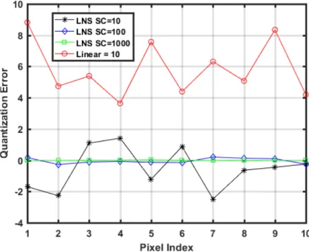
3.5 Comparison between the quantization error for LNS-Q and Linear quan-tization . . . 40

3.6 Comparison between the PSNR for LNS-Q and Linear quantization . . 41

3.7 Mammography Modality : MG-1.dcm . . . 42

3.8 Computer Tomography (CT) and Digital Subtraction Angiography(DS) 43 3.9 X-Ray Angiography (XA)Modality . . . 43

(15)

3.11 Magnetic resonance imaging (MRI) Modality . . . 44

3.12 LNS-DWT experiments methodology and setup . . . 46

3.13 Comparison between the PSNR for Linear Quantization and LNS-Q . . 46

3.14 Comparison between the SSIM for Linear Quantization and LNS-Q . . 47

3.15 Input image . . . 47

3.16 Comparison between the visual effects using linear quantization with different q steps. . . . 48

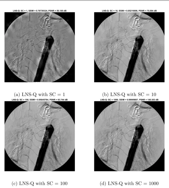
3.17 Comparison between the visual effects with LNS-Q with different SC. . 49

4.1 The integration of LNS-DWT/LNS-Q with WAAVES . . . 52

4.2 An example of converting an image matrix into a vector . . . 53

4.3 Example of a linear DWT dynamic range . . . 53

4.4 Example of a logarithmic DWT dynamic range . . . 54

4.5 The histogram of the linear DWT coefficients after quantization with q = 10 . . . 55

4.6 LNS-DWT histogram with SC = 1 . . . 55

4.7 The Quantized LNS-DWT histogram with SC = 10 . . . 56

4.10 Dynamic range of LL sub band for Linear DWT . . . 58

4.11 Hybrid-DWT compression scheme . . . 58

4.12 Hybrid-DWT construction . . . 59

4.13 Example of scaling the LNS-DWT coefficients without the DRR post filtering (SC = 100) . . . 61

4.14 Scaling the LNS-DWT coefficients (SC = 100) after DRR filter FTH = -12, dynamic range: between -523 and 1250 . . . 61

4.15 Example of the LNS-DWT Coefficients before and after using the DRR filter . . . 62

4.16 The impact of using higher log base on the dynamic range of an input image . . . 63

4.17 Full-LNS Compression scheme with DRR . . . 64

4.18 Experiments Methodology for evaluating the LNS-WAAVES. . . 65

4.19 The impact of changing the logarithm base (NL = 1) . . . 66

4.20 The impact of changing the logarithm base (NL = 4) . . . 67

4.21 CR versus SSIM, Hybrid-DWT with NL = 1 . . . 68

(16)

4.26 CR versus the SSIM improvement, Hybrid-DWT with NL = 3 . . . 71

4.29 DRR Filter impact on the CR with NL = 1 . . . 73

5.1 The global architecture of the proposed unified 2D DWT. . . 77

5.2 The 4-port line buffer architecture. . . 79

5.3 Lifting Predict and Update computation unit (P1U1). . . 80

5.4 Lifting Predict and Update computation unit with scaling (P2U2). . . . 80

5.5 Example of the data representation inside the Line Buffer (LB). . . 81

5.6 Example of H1D Work Buffers data flow. . . 81

5.7 Horizontal 1D Unit (H1D) Top Level. . . 82

5.8 H1D DWT Datapath. . . 83

5.9 H1D Operations sequence and data flow. . . 84

5.10 Vertical 1-D (V1D) Sub block V1D_E/O. . . 85

5.11 The Parallel operation of DMA Read, Write, Horizontal and Vertical DWT via 4 port line buffers. . . 86

5.12 Vertical transform operation sequence and data flow. . . 86

5.13 V1D DWT Datapath. . . 87

5.14 V1D Mode-Initial-Exception operation sequence and data flow. . . 88

5.15 V1D Normal-Mode-operation sequence and data flow. . . 88

5.16 V1D Mode-Final-Exception operation sequence. . . 89

5.17 The proposed DWT coefficients addressing. . . 90

5.18 The fundamentals of Smart EEG telemedicine system. . . 95

5.19 Example coded and decoded frame. . . 96

5.20 Smart EEG experimental prototype. . . 96

A.1 CR versus SSIM, LNS-WAAVES, NL = 4 . . . 107

A.3 CR versus the SSIM improvement, LNS-WAAVES, NL = 4 . . . 108

A.4 CR versus the SSIM improvement, NL = 5 . . . 109

(17)

(18)

1.1 Storage requirements for different medical image Modalities . . . 4

1.2 The required bandwidth to transmit different types of images . . . 4

3.1 LNS object sign cases with examples . . . 27

3.2 List of the tested sample dataset . . . 42

4.1 A comparison between WAAVES using linear DWT and LNS-DWT . . 54

5.1 Lifting coefficients in Fixed-point . . . 79

5.2 Vertical Transform Operations . . . 85

5.3 Altera Stratix IV GX230 resources utilization for 1080p. . . 90

5.4 architecture Scalablity . . . 92

(19)

(20)

Introduction

1.1 Thesis Motivation

Today E-health systems are dominating the medical society thanks to the rapid growth and evolution of the information technology (IT). Hospitals and medical centers depend widely on all the new technologies starting from the simple medical signals measurement devices, e.g. (blood pressure, sugar level, body temperature, electrography, etc.). On the other hand, large medical devices like medical imaging acquisition became an essential tool for radiologists to diagnose diseases [1]. By the time, the continuous increasing in the image resolution and the number of their modalities e.g., (magnetic resonance imaging (MRI), X-Ray, Computed Tomography (CT), ultrasound, etc.) have created many obstacles. That raised the needs to have a huge storage capacity to meet the daily exams archiving requirements, which costs the hospitals heavily.

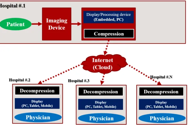
Figure1.1 shows an example of the medical imaging in the eHeath systems 1_.

(21)

Fig. 1.1 Medical imaging in eHeath systems

In addition to that, there are many critical and urgent health problem cases that require radiologists to ask for a diagnostic help from experts who are not in the same hospital at that time. That requires transferring the medical exam via the internet to receive a remote consultation as shown in Figure 1.2.

Fig. 1.2 Remote consultation becomes essential in eHealth today

When sending the medical exams online, the key issue appears in the places that have a limited bandwidth. That makes the upload time is longer and causes a slower

(22)

download speed on the other side. Since the time is a critical factor to save the patients’ lives when they need quick decisions in the emergency cases, it became a big challenge to reduce the transfer and the receive time. Consequently, medical image compression became an essential tool in E-health systems.

In summary, there are several advantages of the image compression in the medical domain that motivated us to explore the challenges and to find the solutions. Image compression helps to reduce the required archiving storage space used in the hospitals, which reduces the storage cost. Also, that makes it feasible to consume less bandwidth when sending and receiving the medical exams, consequently, it reduces the send/receive time via the internet. Finally, it helps in managing the archived medical images faster and more efficient.

1.2 Challenges in the Medical Imaging

Medical image compression became dominant in the medical informatics field. Image compression algorithms that are used in the medical domain provide two types of compressions: lossless and lossy. Although lossless compression provides the perfect reconstruction of the compressed image, it has a limitation in the compression ratio. That is due to the need to preserve more information while performing the compression process [2, 3]. Thus, lossy compression became an interesting topic for the researchers. On the other hand, another challenge is performing the image compression on embedded devices to utilize the device portability feature that enables the availability and the reliability of the remote consultation.

In general, there are the two big challenges in the medical image compression field, which motivated us to work on this research area. They are summarized as the following:

1. The challenge of the compromise between the image quality and the compression efficiency.

2. Compression on embedded systems.

The challenge of the compromise between the image quality and the compression efficiency

Firstly, medical images are vital information, therefore, preserving a sufficient quality on image compression is a critical factor to radiologists to avoid misdiagnoses. Secondly, compression efficiency in terms of the compressed file size is a key element to transfer

(23)

the file in a high-speed, in addtion, to reduce the archiving cost by saving the storage space. However, the main problem appears when compressing with a high compression ratio, which leads to a degradation in the image quality. Table 1.1 lists exsmaples of the storage requirements for different medical exams modalities [4, 5].

Table 1.1 Storage requirements for different medical image Modalities Modality Organ Resolution BPP No. of images Exam Size MRI brain 512 ×512 16 500 250MB abdomen 512×512 16 800 400MB heart 256×256 16 2020 252MB CT brain 512×512 16 500 250MB abdomen 512×512 16 800 400MB heart 512×512 16 2020 1G Angiography Cardiac 1024×1024 8 2000 2G X-ray Chest 2060×2060 16 - 8MB Mammography Breast 4000×5000 12 - 28MB Retinal Eye 2240×1488 RGB,8 - 10MB

Table 1.2 list a comparison between the different image types and the required bandwidth to transmit them [6]. It indicates how the medical images require a large bandwidth compared to the other types of images which is evident that image compression is essential to save the transmit time.

Table 1.2 The required bandwidth to transmit different types of images Size/Duration Transmission

Bandwidth

Grayscale Image 512 × 512 2.1 Mb/image

Colored Image 512 ×512 6.29 Mb/image

Medical Image 2048 × 1680 41.3 Mb/image

Super HD Image 2048 × 2048 100 Mb/image

Full-motion Video 640 × 480,

1 Min (30 frames/Sec) 221 Mb/sec

(24)

• How to achieve an efficient image compression with preserving the diagnostic quality?

Compression on Embedded Systems

Nowadays, radiologists look for the availability of the images anywhere and anytime to give a fast respond diagnose in the emergency cases. Thus, the need of running the compression algorithm on embedded systems became an essential demand. However, embedded systems have many constraints, for example, it has a limited processing speed, and limited memory resources. Therefore, it raises a challenge to adapt the compression algorithm with the available resources on the embedded systems.

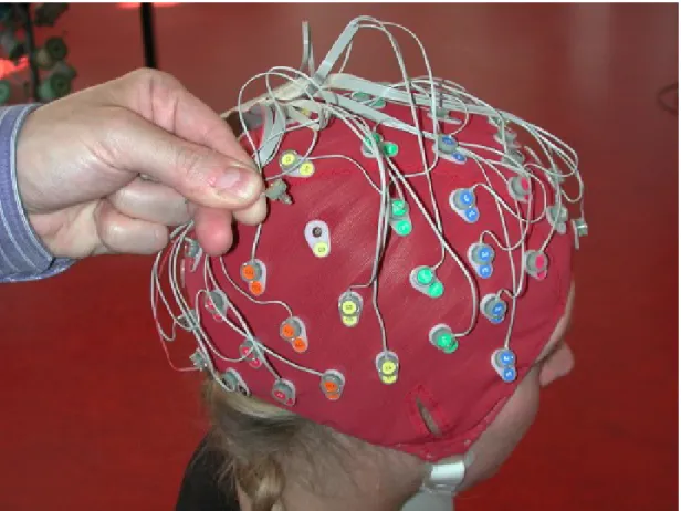
The work presented here is a part of the Smart-EEG project. which is an ongoing telemedicine project aiming to perform remote video EEG exams. Figure 1.3shows the basic idea of this project. Medical signals of a patient, such as EEG (Electroencephalo-gram), ECG (Electrocardiogram) are recorded using an EEG cap as shown in Figure

1.42_{. The EEG signal is combined with the video scene to be compressed, then to be}

sent via the internet to the desired destination. Adding video allows doctors to detect fast myoclonus jerks on the patient. In current systems, the maximum frame rate that can be recorded and transmitted is limited to 30 frame/s. Since the current frame accusation rate is taken every 33ms, this frame rate does not provide a full detection of the myoclonus jerks that requires 10ms which is estimated by 100 frames per second (fps) [7]. To achieve this goal, the video must be in high quality as well as high frame rate. Below this frame rate, doctors are not able to guarantee a trusted detection of the pathology. That took us to another challenge:

• How to adapt the compression algorithm to meet the acceptable speed requirement?

Fig. 1.3 The fundamentals of Smart EEG telemedicine system.

(25)

Fig. 1.4 EEG Cap is used to read the EEG signals

1.3 Thesis Organization

The rest of the thesis is organized as the following:

Chapter Two provides an overview of the background of main elements in the image compression domain. It also reviews the most popular the state of the art image compression algorithms used for medical images. Addition to, it discusses the issues regarding the image quality and what are the preferred metrics for image quality assessment. It also, gives a review of the state of the art of the existing DWT hardware architectures.

Chapter Three It describes the proposed logarithmic-based library and discusses the mathematical issues and the challenges when using the logarithmic arithmetic. It also presents the proposed DWT implementation using the proposed LNS library.

(26)

Chapter Fourprovides analysis of the impact of applying the logarithmic DWT in image compression. Then, it presents the proposed logarithmic DWT-based compression scheme. It also discusses the obtained results when applying the new compression scheme on the medical images, also it gives deep analyses of all the factors that have effects on the compression efficiency.

Chapter Fiveis embedded systems oriented; it proposes a new hardware architec-ture to give a solution to the speed bottleneck on hardware.

Finally, Chapter Six draws the conclusion of the conducted research in this thesis and gives the suggestions for the future work.

(27)

(28)

Background and State of The Art

2.1 Introduction

This chapter covers the concepts and the background of the main elements required to conduct the research. It is organized as the following: Section 2.2 overviews the most popular image compression algorithms that are used in the medical domain. Section2.3

addresses the issues related to the image quality in the image compression algorithms. Section 2.4 discusses the image compression on embedded systems. Finally, in Section

2.5, we draw the conclusion on the issues related image compression.

2.2 Image Compression Algorithms

In this section, we will illustrate the three popular algorithms that are used in medical image applications: JPEG, JPEG2000, and WAAVES.

2.2.1 JPEG

The Joint Photographic Experts Group (JPEG) is a standard image compression algorithm (ISO/IEC 10918) [8, 9]. Its compression flow consists of four stages: first, the color space of input image is transformed from RGB to YCbCr. After that, each color component matrix is divided into blocks of a size 8 × 8 to be processed by the discrete cosine transform (DCT) to generate the DCT coefficients. The output of the DCT stage is quantized using the uniform quantization. The quantized values are encoded using one of the two entropy encoders; Huffman [10] or arithmetic encoder [11]. The JPEG compression flow is shown in Figure 2.1.

Fig. 2.1 JPEG block diagram

The main limitation of the JPEG is the quality degradation when using high quantization step. Also, the segmentation of the input image into blocks of 8×8 pixels that introduces the blocking artifacts [12].

(30)

2.2.2 JPEG2000

Unlike the JPEG which uses the DCT to transform the input image, JPEG2000 uses the DWT instead of it. Although DWT requires more computation time, it eliminates the blocking artifacts. That enhanced the image quality significantly compared to the JPEG. JPEG2000 has two compression modes: lossy and lossless. It uses two different DWT filters: Cohen-Daubechies-Feauveau CDF 9/7 [13] for the lossy compression and the LeGall 5/3 for the lossless compression [14]. JPEG2000 uses an entropy encoder which is based on the arithmetic coding. The compression flow of JPEG2000 is shown in Figure 2.2.

Fig. 2.2 JPEG2000 block diagram

2.2.3 WAAVES

WAAVES [15, 16] is a modern image compression algorithm it was developed by CIRA company [17]. WAAVES accepts RGB color components and transforms them into YCbCr. Also, it supports CMYK (Cyan, Magenta, Yellow, and Black), but in this case, it converts them into RGB, then into YCbCr. Then, the DWT is calculating for each component. WAAVES uses the same DWT filters that are used in JPEG2000. The quantized DWT coefficients are coded using an entropy encoder. WAAVES has an efficient encoder based on Hierarchical Enumerative Coding (HENUC) [18] which gives much better compression than JPEG2000.

Fig. 2.3 WAAVES Compression flow block diagram Compression Algorithms Summary

To summarize, the image compression algorithms are evaluated using three factors: the compression efficiency, the image quality, and the computation complexity.

(31)

JPEG has a better speed than the other compression algorithms since it is based on the DCT. However, it has a limitation in the image quality due to the blocking artifacts. On the other hand, WAAVES is considered better than JPEG2000 in terms of the image quality and the compression ratio [17]. Also, WAAVES is certified for medical applications.

Image compression algorithms are divided into three main stages: an image forward transform (DWT or DCT), a quantization, and an encoding. Since one of the objectives of this work is to explore how to improve the image quality, we started first by investigating the two main sources that affect the image quality: the precision of the arithmetic in the transform stage, and the quantization error. In the next section, we will discuss those issues in details.

2.3 Image Quality Issues in Image Compression

As we stated before, there are two issues that affect the image quality: the arithmetic precision and quantization. We will cover those two topics in this section. Also, we will list the popular image quality assessment metrics and which one of them is suitable for medical imaging applications.

2.3.1 Arithmetic for Digital Signal Processing

Most of the algorithms in digital signal processing (DSP) applications include real number calculations. Thus, there are many data types that give a trade-off between the precision and the computation speed. As we mentioned in the previous section, image compression algorithms include a transform operation on the input image before the encoding stage, e.g. the DWT or the DCT. That transform uses the real numbers during the calculation process. Therefore, the arithmetic precision has an impact on the image quality.

The data representation plays an important role in the computation precision. Depending on the application, we choose the appropriate numerical representation. There are two main number representations: the floating point (FLP) which is suitable for applications that include real number calculation, and; the second type is the fixed-point (FXP) that represents the real data in integer format.

(32)

Floating point

The floating point (FLP) representation is defined in the IEEE 754 [19] with two different word-length formats; the single precision format is 32-bit, and the double precision format is 64-bit. FLP consists of 3 parts: sign bit, exponent, and mantissa. Considering the single precision format [20] as shown in Figure 2.4, there are two possibilities for the dynamic range depending on the exponent value if it is equal zero (denormalized) or not (normalized) as the following:

denormalized: ±2−149 to (1 − 2−23) · 2−126 normalized: ±2−126 to (2 − 2−23) · 2127

Fig. 2.4 Single precision FLP format (32-bit)

The last decade, many publications addressed the usage of the floating-point in many applications that require higher accuracy than fixed-point (single precision), [21–28]. Also, several publications addressed the double precision [29–32].

Fixed point

The second data type is the fixed point (FXP) format, which is used as an alternate to the floating-point. Because the calculation using FLP is expensive and slow. FXP is considered an attractive candidate for DSP algorithms implementation on hardware. That is due to its simplicity which gives faster spped for the arithmetic operations. However, FXP has a limitation regarding the dynamic range that affects the accuracy. As shown in Figure 2.5 a W-bit FXP consists of three parts: the sign bit, the integer part wi, and the fractional part wf, where w = 1 + wi+ wf and its dynamic range is described in equation (2.1) [33].

(33)

−2wi _{≤ x <}2wi (2.1)

Logarithmic Number System

The logarithmic number system (LNS) has been recently introduced in the literature [34–37] as an alternative solution to the floating-point. It also can provide a high precision and a wider dynamic range than the fixed-point. LNS is an interesting research area because it gives a simple implementation of the multiplication, division, square root and square of numbers. Although the addition and the subtraction operations in LNS are complicated, many publications have presented that LNS can achieve a higher performance than floating-point [35, 38]. Due to the raising of the interest in the LNS research area, an LNS library has been introduced by [39]. The main objective of that library is to provide a tool for the purpose of the comparison with the fixed-point format on hardware in terms of speed and accuracy.

The LNS format is inherited from the fixed-point representation. Although there is no standard to define the format as the IEEE FLP, however, the LNS format in [40] [36] is commonly used. LNS is defined in Figure 2.6[36]. The exponent value for the base 2 is described as in equation (2.2):

X= (−1)s×2m.f (2.2)

where s is the sign bit, m is the integer part, f is the fractional part.

Fig. 2.6 32-bit LNS format

The LNS 2-bit dynamic range is between 2−128 _{to 2}128_{, which is near to the}

(34)

Logarithmic Number System Arithmetic

Performing computations in LNS requires converting the input data to the logarithmic domain by computing their logarithm. Assuming that there are two numbers x and y in the linear domain (real world values) and their logarithmic representations are a and b respectively, where x ≥ y are as follows:

a= log(|x|) (2.3)

b= log(|y|) (2.4)

The basic LNS arithmetic operations on x and y using the signed logarithmic format [36] [41] are listed as the following:

Multiplication: log(x × y) = a + b (2.5)

Division: log(x ÷ y) = a − b (2.6)

Addition: log(x + y) = b + log(2a−b_{+ 1)} _(2.7)

Subtraction: log(x − y) = b + log(2a−b₋₁₎ _(2.8)

As described in equation (2.5) and equation (2.6), the main advantage of the LNS arithmetic is simplifying the multiplication and division operations by converting them into addition and subtraction operations respectively. On the other hand, as shown in equation (2.7) and equation (2.8), the addition and subtraction operations became a challenge in the LNS domain. Since they require nonlinear functions that involve a logarithm and an exponent operation that make their computation is complex.

Choosing between the LNS or the FXP representation depends on the algorithm. Hence, to take the advantage of the logarithmic arithmetic, the number of the multipli-cation and the division operations has to be larger than the number of the addition and the subtraction operations. The reason of that is the number of addition and subtraction operations has a negative impact on the overall speed. That is because they contain additional logarithmic calculation.

In summary, the main goal of the published LNS arithmetic in the literature is to provide an alternative representation to the fixed-point to achieve high-performance hardware architectures with a better precision. In contrast, the main aim in this

(35)

context is to explore if the LNS arithmetic is used as an alternate to the FLP can improve image compression algorithms due to its data compactness feature with a precision similar to the FLP.

2.3.2 Uniform Quantization

The quantization is the main source of the quality degradation in the image compression. However, it is an essential process because it reduces the dynamic range and converts the DWT coefficients from real numbers to integers. That is because the encoder works only on integer values. The quantization process is achieved by dividing the DWT outputs by a quantization step. Using a large value of the quantization step gives a better compression ratio, but it leads to a low image quality. The quantization process is defined in equation (2.9) [42] [43] as the following:

Xq = sign(X)⌊

X

q ⌋ (2.9)

where X is the DWT coefficients, Xq is the quantized coefficients with a quantization

step q.

2.3.3 Image Quality Assessment

Image quality assessment is an essential process to evaluate image processing algorithms. In this context, the main objective of using the quality assessment is to evaluate the compression algorithms. In the literature, there are many quality metrics that are used to evaluate the image quality. The most popular metrics are: the peak signal-to-noise ratio (PSNR) and the structural similarity index (SSIM). Both metrics requires the original image as a reference to be compared with the reconstructed image after decompression.

The PSNR between the original and the reconstructed image is defined in (2.10), it is widely used as an image quality metric. Recently, it has been shown by researchers that PSNR is not a sufficient metric to assess the image quality because it depends only on the mean square error (MSE)[44].

P SN R(dB) =log10(I

2₎

√

M SE (2.10)

(36)

M SE= 1 M N N X i=1 M X j=1 (Fi,j− Gi,j) (2.11)

where M,N are the image dimensions, F,G are the reference and the reconstructed image respectively, (i,j) is the pixel location in the image matrix.

On the other hand, the structural similarity index (SSIM) [45, 46] is considered as more appropriate metric for evaluating the visual performance since it measures the image in terms of the human visual system components: structural, luminance and contrast between two images. Due to these reasons, radiologists are moving towards considering the SSIM as an alternative to the PSNR metric [47] for the image quality assessment. The SSIM is defined in equation (2.12).

SSIM(f,g) =(2µfµg+ C1) + 2σfσg+ C2

(µ2

fµ2g+ C1)(σf2σ2g+ C2) (2.12)

where f and g are the original and reconstructed images, respectively, µf , µg are the mean

intensity values for the two images f and g respectively, σf, σg are the standard deviation of

the two images and C1 , C2 are constants.

2.4 Acceleration on Embedded Systems

As we described in the previous chapter, one of the main objectives of the Smart-EEG project is to build a portable medical device that can compress up to 100 frames/s. WAAVES was chosen for the project to be implemented due to its compression and image quality efficiency. Since the WAAVES HENUC encoder module was implemented by the team in LIP6 [48], the DWT module is the only targeted part in the compression algorithm that will be covered in this work.

In this section, we provide a description of the popular DWT algorithms. After that, we highlight the different embedded systems platforms that are suitable for image compression algorithms. Then, we review the related work of the DWT implementation on embedded systems.

2.4.1 Discrete Wavelet Transform

DWT is an essential stage in the compression chain in many image compression algorithms such as WAAVES and the JPEG 2000. One of the key advantages of the DWT-based compression is providing a multi-resolution transform and giving an analysis in the spatial

(37)

frequency and the location. In contrast to the Discrete Cosine Transform (DCT) which is used in JPEG, DWT provides better image quality and compression.

The 2D-DWT flow has two stages: In the first stage, the 1D-DWT is applied along the image rows to perform the horizontal DWT. That splits the image into low (L) and high (H) frequency sub-bands. In the second stage, another 1D-DWT (Vertical transform) is applied to the output of the horizontal DWT to obtain the four sub-bands (LL, LH, HL, HH) coefficients. Figure 2.7 shows the 2D-DWT computation flow. In image compression, the image requires a multi-level 2D-DWT. That is achieved by applying the 2D-DWT to the LL sub-band. That process is repeated for the required number N of 2D-DWT levels depending on the image size. An example of applying the 2D-DWT on a medical image is shown in Figure 2.8.

Fig. 2.7 The 2D DWT computation flow

(a) input image before DWT (b) DWT decomposition Fig. 2.8 Example of an 2D-DWT for a medical image

There are two popular DWT algorithms: Filterbank-based DWT and Lifting scheme, we describe them in the following two sections.

Filter Bank (Convolution)

The convolution based DWT consists of two perfect-reconstruction (PR) finite impulse response (FIR) filter banks: lowpass H(z) and highpass G(z). They are followed by a down

(38)

sampling operation that iis applied to their outputs. That yields a low band xl and a high

band xh for the input x(n). Figure 2.9shows a block diagram of the convolution based DWT.

The main limitation of this structure requires is the computation time. That is because there is a wasted time due to the filtering operation to all the samples, then applying the down sampling operation. The down sampling means discarding half of the samples that were computed from the previous filtering stage [49].

Fig. 2.9 Block diagram of convolution based DWT.

xl(n) = l X i=0 h(i)x(2n − i) (2.13) xh(n) = m X i=0 g(i)x(2n − i) (2.14)

where, l and m are the lengths of the lowpass and highpass filters respectively.

To calculate the 2D-DWT, let x(n) is a row in the input image. The horizontal transform is calculated by applying the lowpass H(z) and highpass G(z) to each row. For the vertical transform, x(n) is considered the column in the output of the horizontal transform; it is passed to the two filters. To calculate the multi-level 2D-DWT, each row in the output of the lowpass filter of the vertical is considered x(n) and so on.

Lifting Scheme

The second approach to compute the DWT is the lifting scheme. Its main idea is to decompose the filter bank into a sequence of lifting steps [50–52]. Looking to the polyphase filter matrix

p(z) in the equation (2.15) which includes the low pass filter h(z) and the highpass filter g(z)

in the equation (2.16) and the equation (2.17) respectively. The matrix p(z) is factorized into a series of upper and lower triangular matrices is called the lifting steps as described

(39)

in the equation (2.18). The described filter in the equation (2.18) is the bi-orthogonal Cohen-Daubechies-Favreau (CDF) 9/7 filter bank which is used in both lossy compression algorithms (WAAVES and JPEG2000).

p(z) = " he(z) ho(z) ge(z) go(z) # (2.15) h(z) = he(z2) + z−1ho(z2) (2.16) g(z) = ge(z2) + z−1go(z2) (2.17)

where he(z) and ge(z) are the even parts and ho(z) and go(z) are the odd parts of the

lowpass h(z) and highpass g(z) filters respectively.

p(z) = " 1 α(1 + z−1₎ 0 1 # " 1 0 β(1 + z−1) 1 # × " 1 γ(1 + z−1₎ 0 1 # " 1 0 δ(1 + z−1) 1 # " k 0 0 1 k # (2.18) where the CDF 9/7 filter coefficients values are:

α= −1.586134342 β = −0.05298011854 γ= 0.8829110762 δ= 0.4435068522 K= 1.149604398

Figure 2.10 shows the block diagram of the DWT lifting scheme. It includes four steps: (1) split, (2) predict, (3) update, and (4) scaling.

(40)

The detailed mathematical description of the lifting scheme algorithm for the 9/7 CDF filter is listed in the equations (2.19)-(2.26). The signal x is split into odd dn

i and even sni

parts, where n is the lifting step number. Each step consists of predict and update, the last stage is a scaling step:

Spilt stage:

Odd: d0_i = x2i+1 (2.19)

Even: s0

i = x2i (2.20)

First lifting step:

Predict 1: d1_i = d0_i+ α(s0_i+ s0_i+1) (2.21)

Update 1: s1_i = s0_i+ β(d1_i−1+ d1_i) (2.22)

Second lifting step:

Predict 2: d2 i = d1i+ γ(s1i+ s1i+1) (2.23) Update 2: s2_i = s1_i+ δ(d2_i−1+ d2_i) (2.24) Scaling step: Odd scaling: di=d 2 i k (2.25) Even scaling: si= s2i× k (2.26)

There are many advantages of the lifting scheme; (1) it requires less number of multipli-cation and addition operations than the convolution based approach; (2) the lifting scheme consumes less memory space thanks to the in-place calculation feature, that is because input data is updated and is overwritten by the output of the lifting stages; (3) the transform is a simply revisable, to calculate the inverse of the DWT, it requires only to reverse the lifting steps by performing them backwards (scaling, update, predict). [53, 51].

2.4.2 Embedded Systems Platforms

There are a variety of embedded system platforms depending on the targeted application [54]. In general, we can divide the embedded systems according to the processing speed and the development time. In general, there are three popular solutions: DSP, FPGA, and ASIC.

DSP

Digital signal processors (DSPs) are considered much faster and have higher performance than Microcontrollers. The main advantage of DSPs, they include hardwired functions that are used in the signal processing algorithms. They also, has a higher clock speed, optimized instruction set, and memory organization.

(41)

FPGAs

Field programmable gate arrays are reconfigurable hardware circuits according to the required application. The register transfer language (RTL) is used to describe the targeted algorithm. There are two commonly used RTL languages: VHDL and Verilog. Since everything is implemented on hardware, FPGAs are considered a perfect solution for high-speed processing requirements, they also require reasonable development time.

ASICs

Application-specific integrated circuit (ASIC) are circuits that are dedicated for a specific application. There is no possibility of the reprogramming or the reconfiguration after the manufacturing. Hence, it requires longer development time. However, in terms of performance, it can reach a higher speed than FPGA according to the design. RTL is used to describe the architectures.

2.4.3 Previous Implementation of the DWT on Embedded

Sys-tems

There are several existing DWT architectures in the literature. They exist in different technologies: FPGAs and ASICs. DWT architectures read the image data with one of the three scanning schemes, line-based [55, 56], block-based [57] or stripe-based [58].

In terms of control path complexity and memory requirements. Lifting-based DWT architectures are divided into three categories: folded [59, 60], parallel [61–63] and recursive [51, 64, 65]. Darji et al. [65] proposed three different architectures based on the folded multi-level architecture (FMA), pipelined multi-multi-level architecture (PMA) and recursive multi-multi-level architecture (RMA).

Dual-scan and clock gating techniques were used to increase the throughput and minimize the on-chip frame line buffers. Aziz and Pham [62] presented a parallel 2D-DWT multiplier-free architecture with a high operating frequency by replacing the multiplications by shift operations.

A unified FPGA-based architecture for 2D DWT was proposed by Sameen at al [66], it included a Nios II soft-core processor with attached hardware accelerators giving a high throughput and a real-time capability for gray-scale video processing with a full HD resolution.

A memory-efficient convolution-based 2D DWT architecture was introduced by Mohanty et al. [57]. Their architecture involved more multipliers than the existing ones, but it requires less memory. They synthesized their architecture for 90nm ASIC implementation. Hu and Jong [67] proposed another parallel lifting-based 2D DWT scalable architecture which requires less memory. They synthesized the design for ASIC with a 90-nm technology. Hu and Jong

(42)

[58] introduced another parallel 2D DWT architecture based on a stripe scanning method which gives high throughput and requires less temporal memory.

After the analysis of the related work, we concluded that most of the high throughput DWT architectures do not meet the requirements of the Smart EEG-project. There is no existing architecture support 100 frame/s and taking in consideration the latency of the double data rate random access memory (DDR RAM).

2.5 Discussion and Conclusion

In this chapter, we reviewed the famous image compression algorithms that are used in medical image applications. WAAVES is considered better than JPEG and JPEG2000 since it compresses images more efficiently and reconstructs them with a better quality.

We also discussed the two issues that have an influence on the image quality: the arithmetic and the quantization. For the arithmetic, floating point (FLP) and logarithmic number system (LNS) are considered better than fixed point (FXP), since they provide a high precision. LNS has a similar dynamic range to the FLP, and it also has the data compactness feature. That gives it another advantage which attracted us to investigate the possibility of utilizing it in the image compression applications.

Also, we explored the image quality assessment metrics. According to the literature, the PSNR is not sufficient to evaluate the image quality, while the SSIM is used as an alternative because it measures the visual properties in the image.

The second objective of our work is the image compression on embedded systems as a part of the Smart-EEG project. In this context, we investigate the DWT implementation on hardware since the other compression modules have implemented previously. We started by exploring the two DWT algorithms, and we found that the lifting scheme has many advantages over the convolution approach regarding its computation efficiency and memory requirements. Between the different embedded systems platforms, we concluded that the FPGA is considered as the best solution for prototyping the targeted application. That is because the development time is significantly shorter than ASIC. It is also cheaper, since it is reconfigurable, so the modification in the design does not require to fabricate the chip again.

We also provided a review of the existing solutions for accelerating the DWT on embedded systems. We found that most of the existing architectures did not consider the DDR ram latency which is the main bottleneck. Since the previous work did not meet the Smart-EEG requirements, it motivated us to investigate how to fulfill the Smart-Smart-EEG prototype requirements.

In summary, the main objective of this work is to find the answers to the following problematic research questions:

(43)

1. Does the logarithmic representation has the ability to improve the compro-mise between the compression ratio and the image quality?

2. How to provide a new DWT hardware architecture that can fulfill the Smart-EGG high-speed requirement?

(44)

Logarithmic-Based Discrete

Wavelet Transform

3.1 Introduction

As we stated in the previous chapter, preserving the diagnostic quality of the medical images is the main aim of this work. Therefore, we raised the research question; if changing the arithmetic domain can improve the quality of the reconstructed images after the compression.

(45)

In this chapter, we investigate switching the calculation from the linear to the logarithmic domain. In addition, evaluating the logarithmic arithmetic demanded that we build a custom logarithmic-based software library that we present in this chapter.

This chapter is organized as the following: In Section 3.2 we present and discuss the proposed logarithmic Library (LNS-LIB) and the mathematical issues related to the loga-rithmic domain. Section 3.3 discuss the LNS-LIB validation phases. Section 3.4 presents the logarithmic DWT using LNS-LIB. Section3.5presents the new logarithmic quantization method and provides a comparison with the linear quantization method. Section3.6describes the used dataset and the conducted experiments. Section 3.7discusses the obtained results. Finally, in Section3.8, we draw the overall conclusion for the presented work in this chapter.

3.2 LNS Library Implementation

This section present the LNS custom library we developed to ease the implementation of algorithms in LNS arithmetic. This library was built using MATLAB software, and it consist of two parts: the definition of the LNS object format (see section3.2.1) and the functions that implement the four arithmetic operators (see section3.2.2).

3.2.1 LNS Data Object Definition

The LNS data object is defined as a container that holds the logarithmic data. Let x be a real number in the linear domain, then, the LNS data object L is defined according to the equation (3.1), where L contains two elements: the logarithmic value field v with base B and the sign flag s.

LNS-Object L = {v,s} (3.1)

Notation of the LNS-Object Data Structure

For an LNS-object, we use dot (.) operator in the notation (.v) and (.s) to access the value field and the sign flag respectively. For example, the value field in the LNS-object L can be accessed using the notation L.v, and in the same manner for sign flag using L.s.

Data Handling Issues

There are two issues related to the properties of the logarithmic function f(x) = log(x): 1. The logarithm of a negative number is undefined.

(46)

These two issues must be taken into consideration when converting the data from the linear to the logarithmic domain. Therefore, we introduce two solutions to handle them: the

sign flag and the virtual zero.

The Sign Flag

Regarding the first issue, since the logarithm of a negative number is undefined. Thus, we must take the logarithm of the absolute value. However, this causes a phenomena known as the sign ambiguity. This happens because the LNS domain contains two sources of a negative sign.

1. The first case: if the value of x lies in the range of (0 < x < 1), then, its logarithm (log(x)) yields a negative value.

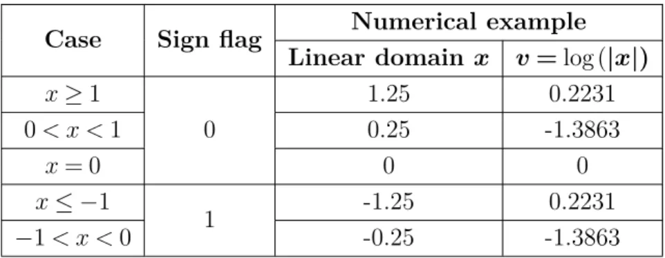
2. The second case: if x is a negative (x < 0), then, its logarithm (log(|x|)) yields a negative value if it lies within the range (−1 < x < 0), or a positive value otherwise. As a consequence of the previous two cases, the negative sign in the logarithmic domain is not enough to indicate if the linear value was originally negative or not. Hence, it raised the importance of the sign flag which has the purpose to resolve the sign ambiguity. Table

3.1lists all the cases for the sign flag of an LNS-object. As shown in the example listed in Table3.1, the x values 0.25 and −0.25 have the same logarithmic value −1.3863. However, thanks to the sign flag, we can distinguish between them.

Table 3.1 LNS object sign cases with examples Case Sign flag Numerical example

Linear domain x v =log(|x|) x ≥1 0 1.25 0.2231 0 < x < 1 0.25 -1.3863 x= 0 0 0 x ≤ −1 1 -1.25 0.2231 −1 < x < 0 -0.25 -1.3863

The Virtual Zero

Concerning the second issue related to the fact log(0) = −∞, we handled it by introducing a new feature in the LNS-Library called the virtual zero. We define the virtual zero as following:

"The zero value in the logarithmic domain is originally a zero value in the linear domain."

In other words, when converting x = 0 from the linear domain to the logarithmic domain, we keep it zero without applying the logarithm operation. Equation (3.2) describes the

(47)

virtual zero concept. We set the data field of an LNS-object to zero (L.v = 0) if (x = 0). The sign flag is described in equation (3.3).

L.v=    log(|x|) x ̸= 0 0 x= 0 (3.2) L.s=    0 x ≥0 1 x <0 (3.3)

The virtual zero feature gives the library two advantages: (1) image processing compati-bility; since virtual zero makes the LNS library able to convert an input image containing zeros to the logarithmic domain. (2) optimizing the logarithmic arithmetic operations; since they resembles the linear domain when handling the zeros (see in Section3.2.2).

Logarithmic to Linear Conversion

To convert back an LNS-object L to its linear representation x, we use the exponent function to calculate the inverse of the logarithm as defined in equation (3.4). The virtual zero and the sign flag L.s are handled in the conversion operation.

x=    −1L.s_{× B}L.v _{L.v ̸}_{= 0} 0 L.v= 0 (3.4)

The library also handles the true zero, which occurs when log2(x) = 0 with x = 1. It simply

replaces the x = 1 with the nearest value. For example X is replaced with 1.00000000001, therefor, Log2(1.00000000001) = 1.4427 × 10−11which is a very small value that nearly equal

zero. The reason for using this is to distinguish between the virtual and the true zero. The library gives a priority to the virtual zero since it was oriented for image processing applications.

3.2.2 LNS Arithmetic Operators

The second part of the LNS library is the arithmetic operators. The basic four operations (multiplication, division, addition, and subtraction) were implemented as the following:

(48)

LNS Multiplication and Division

The function LNS_MulDiv as shown in equation (3.5) performs the multiplication and division for A = {v,s} and B = {v,s} respectively. It returns the result into an LNS object

C= {v,s}. The function is based on the equation (2.5) and the equation (2.6) respectively

presented in Chapter2.

C= LNS_MulDiv(A,B,MD) (3.5)

The function accepts three input parameters: the two LNS-objects and a 1-bit flag parameter MD. The value of MD defines the type of the operation. If MD = 0, then a multiplication operation will be performed. Otherwise, if MD = 1, then a division operation is performed. The function output has three possible results as indicated in equation (3.6). The output can be zero if the value of one of the inputs or both of them are equal to zero. Hence, the virtual zero gives us the advantage of treating these operations in a way similar to that in the linear domain.

C.v=          0 A.v= 0 or B.v = 0 A.v+ B.v M D= 0 A.v − B.v M D= 1 (3.6)

Regarding the sign flag as shown in equation (3.7), the output sign remains the same if both inputs have the same sign. On the other hand, the output sign flag is set to 1 if the inputs have a different sign, which is similar to the linear multiplication/division.

C.s=          0 A.v= 0 or B.v = 0 0 A.s= B.s 1 A.s ̸= B.s (3.7)

LNS Addition and Subtraction

The function LNS_Add performs the addition and the subtraction operations for two LNS-objects A and B respectively. It returns the result into an LNS-object C as shown in equation (3.8).

(49)

The value of the fields C.v and sign flag C.s of resulted LNS-object C are defined in equation (3.9) and equation (3.10) respectively. These operations are based on equation (2.7) and equation (2.8) that were mentioned in the previous chapter.

C.v=                             

A.v+ f_add A.s= B.s A.v+ f_sub A.s ̸= B.s

A.v B.v= 0

B.v A.v= 0

0 A.v= B.v and A.s ̸= B.s

0 A.v= B.v = 0 (3.9) C.s=    A.s A ≥ B B.s A < B (3.10)

The nonlinear functions f_add and f_sub are defined in equation (3.11) and equation (3.12) respectively.

f_add = log(1 + 2B.v−A.v) where A > B (3.11)

f_sub = log(1 − 2B.v−A.v) where A > B (3.12)

There are five possible result values for C.v depending on the input values of A and B. The results are calculated using the similar principles of the addition in the linear domain. The addition is performed using the function in equation (3.11) if the sign fields of both inputs are the same. Otherwise, if the sign fields of both inputs are different, the subtraction is performed using the function in equation (3.12).

On the other hand, there are two special cases related to the virtual zero. The first case occurs when one of both inputs is virtual zero. Therefore the result is the non-zero input. The second case occurs when both inputs are virtual zeros; then the result is a virtual zero. In summary, if the inputs contain a virtual zero, the operator becomes an assignment, this limits the overhead of the addition and subtraction operations that resulted from the nonlinear functions f_add and f_sub. That is an interesting aspect of the library because introducing the virtual zero decreases the computation time. In other words, having more zeros leads to less addition/subtraction operations.

(50)

Example3.1 gives a numerical example of how the functions are used to calculate the addition/multiplication.

H Example 3.1.

Let x= 3.5 and y = −2.5, Then, their addition is:

z= x + y = 1, and their multiplication is: w= x × y = −8.75.

To perform the same operations in LNS, first we convert x and y to LNS-objects

xl and yl, as the following: xl= {v,s} = {1.8073,0}, and yl= {v,s} = {1.3219,1}

then, the addition of the two number in LNS is: zl= LNS_add(xl, yl)

zl= {v,s} = {−4.44089×10−16,0}, which yields 1 when converting back zl to the

linear domain and the multiplication of the two number in LNS is: wl= LNS_MulDiv(xl, yl,0)

wl= {v,s} = {3.1292,0} which yields −8.75 when converting back zl to the linear

domain.

3.3 Library Validation

Fig. 3.1 The validation methodology of LNS-Library operators

The LNS library was validated by performing a set of verification test phases. The first test phase objective was to validate the four basic mathematical operations (addition, subtraction,

(51)

multiplication, and division). The operations were tested in the logarithmic domain. Then their results were converted back to the linear domain. These converted results are compared to golden reference values. A description of the first phase of the validation is shown in Figure 3.1.

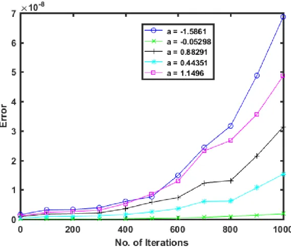
The second validation process was done by performing the multiply and accumulate (MAC) operation. The MAC operation is described in equation (3.13). The MAC was chosen because it combines two operations, which is similar to the calculation behavior in many image processing algorithms. The purpose of this phase was to measure the error ϵ between the linear Mlin and the logarithmic domain Mlns for different n iterations of MAC

as described in equation (3.14). M= n X i=0 a × i (3.13)

where, M is the total of multiplying i by a constant a.

ϵ= |Mlin− Mlns| (3.14)

where, ϵ is the absolute error, Mlin is the MAC output in the linear domain, and Mlns is the

MAC output in the logarithmic domain.

Figure3.2shows the absolute error for different MAC iterations with different constants. The constants of the lifting DWT 9/7 CDF filters were chosen in the MAC experiment since the main aim of the LNS Library is to be used for the DWT implementation. The results show that the error was increased when calculating an enormous number of iterations. However, the error was still slightly small, since it reached around 7×10−8 _{at 1000 iterations.}

In conclusion, this evaluation indicates that the library is reliable regarding the accumulated error.

(52)

Fig. 3.2 Error between linear and logarithmic for MAC using different constants

3.4 Discrete Wavelet Transform using The LNS Library

The discrete wavelet transform (DWT) is considered as the backbone of modern image compression algorithms. The DWT performs the image processing part as a first phase in the compression algorithm before the coding phase. After the first validation of LNS library, this section investigates the DWT implementation using the logarithmic arithmetic as an alternative to the linear arithmetic.

According to the state of the art, there are two approaches for DWT implementation: convolution based and lifting based approaches. In this work, the DWT lifting scheme has been chosen because of its efficiency in terms of computation and memory requirements [53]. We selected the DWT-based 9/7 CDF filter to be implemented in LNS since it is used in WAAVES and JPE2000 [16].

The 2D-DWT implementation in the logarithmic domain consists of two basic steps as listed in Algorithm 1: The first step is to convert the input image from the linear to the logarithmic domain. After that, we calculate the 1D-LNS-DWT for each line in the

(53)

logarithmic image, yielding the horizontal DWT-coefficients matrix. Finally, we calculate the vertical transform for each line in horizontal DWT-coefficients matrix.

Algorithm 1: 2D LNS-DWT

Input : A logarithmic image LI, Width, High Output : 2D LNS-DWT Coefficients V

1 for L = 0 to Hight-1 do // 1D DWT horizontal transform for each image line 2 H(L) = 1D LNS-DWT of LI(L)

3 end

4 for C = 0 to Width-1 do // 1D vertical transform for each column

5 V(C) = 1D LNS-DWT of H(C) 6 end

The 1D-DWT transform was implemented using LNS library based on the equations from (2.19) to (2.26) as presented in Chapter 2. Its implementation is divided into six parts which are described in the algorithms from Algorithm 2 to Algorithm8. The first stage in the 1D-DWT is the Predict-1 which works on the even elements in the input line X. For each odd element X_current, the previous element X_prev and the next element X_next are added then multiplied by the constant α. Then, the multiplication output is added to that X_current yielding the Predict-1 output P 1 as described in equation (3.15):

P1 = X_current + alpha × (X_prev + X_next) (3.15)

The next stage is the Update-1 which is similar to the Predict-1, it works on the odd elements on the input line X and the output of the Update-1. The next stage of the computation includes the Predict -2 followed by the Updated-2 stage. Both are calculated in the same manner like Update -1 and Predict-2 but with changing the filter constants. The output of both previous stages is scaled, then packed together to form the final output of the 1D-DWT transform.

(54)

Algorithm 2: 1D-DWT LNS : Part 1 - Lifting stage Predict 1

Input : X , N // one line of an image

Output : Y // Y = 1D_DWT_LNS(X)

// Where X is an input vector LNS object type with a length N // Predict 1: X_next = X_current + alpha*(X_prev + X_next)

1 for i = 1 to N-1 step 2 do // odd values

2 ADD = Add_LNS(X(i-1) , X(i+1) ) 3 MUL = Mul_LNS(alpha, ADD) 4 P1(i) = Add_LNS(X_current , MUL) 5 end

Algorithm 3: 1D-DWT LNS: Part 2 - Lifting stage Update 1

// Update 1: X_next = X_current + Beta *(X_prev + X_next)

1 for i = 0 to N-1 step 2 do // even values

2 ADD = Add_LNS(P1(i-1), P1(i+1)) 3 MUL = Mul_LNS(Beta, ADD) 4 U1(i) = Add_LNS(P1(i) , MUL_1) 5 end

Algorithm 4: 1D-DWT LNS: Part 3 - Lifting stage Predict 2

// Predict 2: X_next = X_current + Delta *(X_prev + X_next)

2 ADD = Add_LNS(U1(i-1), U1(i+1)) 3 MUL = Mul_LNS(Delta, ADD) 4 P2(i) = Add_LNS(P1(i) , MUL) 5 end

(55)

Algorithm 5: 1D-DWT LNS: Part 4 - Lifting stage Update 2

// Update 2: X_next = X_current + Gama *(X_prev + X_next)

2 ADD = Add_LNS(P2(i-1) , P2(i+1)) 3 MUL = Mul_LNS(Gama, ADD)

4 U2(i) = Add_LNS(U1_current , MUL_3) 5 end

Algorithm 6: 1D-DWT LNS: Part 5-A - Lifting stage Scaling odd elements

// Lifting Scale :

2 P2S(i) = Mul_LNS(P2(i), Z0) 3 end

Algorithm 7: 1D-DWT LNS: Part 5-B - Lifting Stage Scaling even elements

2 U2S(i) = Mul_LNS(U2(i), Z1) 3 end

Logarithmic Discrete Wavelet Transform For High Quality Medical Image Compression

HAL Id: tel-02085662

https://tel.archives-ouvertes.fr/tel-02085662v2

Quality Medical Image Compression

Mohammed Shaaban Ibraheem

To cite this version:

DE L’UNIVERSITÉ PIERRE ET MARIE CURIE

Spécialité : Informatique

École doctorale :

EDITE 130 Paris

à LIP6

Mohammed Shaaban IBRAHEEM

DOCTEUR DE L’UNIVERSITÉ PIERRE ET MARIE CURIE

Logarithmic Discrete Wavelet Transform for High

Quality Medical Image Compression

Introduction

Contents

1.1

Thesis Motivation

1.2

Challenges in the Medical Imaging

1.3

Thesis Organization

Background and State of The Art

Contents

2.1

Introduction

2.2

Image Compression Algorithms

2.2.1

JPEG

2.2.2

JPEG2000

2.2.3

WAAVES

2.3

Image Quality Issues in Image Compression

2.3.1

Arithmetic for Digital Signal Processing

2.3.2

Uniform Quantization

2.3.3

Image Quality Assessment

2.4

Acceleration on Embedded Systems

2.4.1

Discrete Wavelet Transform

2.4.2

Embedded Systems Platforms

2.4.3

Previous Implementation of the DWT on Embedded

Sys-tems

2.5

Discussion and Conclusion

Logarithmic-Based Discrete

Wavelet Transform

Contents

3.1

Introduction

3.2

LNS Library Implementation

3.2.1

LNS Data Object Definition

3.2.2

LNS Arithmetic Operators

3.3

Library Validation

3.4

Discrete Wavelet Transform using The LNS Library