"Two-Sided Wealth Constraints and Innovation Adoption: Evidence from a Grassroot Extension Programme in Peru"

RESEARCH OUTPUTS / RÉSULTATS DE RECHERCHE

Author(s) - Auteur(s) :

Publication date - Date de publication :

Permanent link - Permalien :

Rights / License - Licence de droit d’auteur :

Bibliothèque Universitaire Moretus Plantin

Dépôt Institutionnel - Portail de la Recherche

researchportal.unamur.be

"Two-Sided Wealth Constraints and Innovation Adoption: Evidence from a Grassroot Extension Programme in Peru"

Platteau, Jean-Philippe; Bonjean, Isabelle; Verardi, Vincenzo

Publication date: 2009

Document Version

Early version, also known as pre-print

Link to publication

Citation for pulished version (HARVARD):

Platteau, J-P, Bonjean, I & Verardi, V 2009 '"Two-Sided Wealth Constraints and Innovation Adoption: Evidence from a Grassroot Extension Programme in Peru"'.

General rights

Copyright and moral rights for the publications made accessible in the public portal are retained by the authors and/or other copyright owners and it is a condition of accessing publications that users recognise and abide by the legal requirements associated with these rights. • Users may download and print one copy of any publication from the public portal for the purpose of private study or research. • You may not further distribute the material or use it for any profit-making activity or commercial gain

• You may freely distribute the URL identifying the publication in the public portal ? Take down policy

If you believe that this document breaches copyright please contact us providing details, and we will remove access to the work immediately and investigate your claim.

Two-Sided Liquidity Constraints and Innovation

Adoption: Evidence from a Grassroots Extension

Programme in Peru

by

Isabelle Bonjean, Jean-Philippe Platteau and Vincenzo Verardi

Centre of Research for Development Economics (CRED) Department of Economics, University of Namur

Rempart de la Vierge 8 B-5000 Namur Belgium

Abstract. Our study uses a quasi-natural experiment to assess the presence of wealth

constraints limiting both demand for and supply of technical innovations adapted to cattle herders in a poor and remote area of the Peruvian Highlands. This is done in the context of a specific NGO intervention aimed at activating a market for such innovations through the channel of grassroots extension agents. Unique features of our dataset are (i) the highly disaggregated characterization of innovations, and (ii) detailed information about providers of agricultural extension. We show that significant liquidity constraints exist on the two sides of the market, and that innovation adoption is significantly influenced by participation in training events but only provided that these constraints are overcome. Moreover, economic viability of grassroots agents is shown to hinge critically on their combination of extension and productive activities.

May 2012

* _{We want to express our gratitude to the Non-Governmental Organisation “SP Soluciones Practicas, Peru” for} their continuous support to the data collection process without which the present study would not have been possible. This support took two forms: allowing Isabelle Bonjean to have access to a dataset gathered by the NGO itself, and helping her, both in terms of logistics and communication, to enter the sample communities in order to collect fresh complementary data. Our thanks are due to Carlos de la Torre and Daniel Rodriguez (posted in Lima), and to the staff persons posted in Cajamarca, Maria Sol Blanco, Nestor Fuertes, Miguel Malaver, Ines Pando, Roger Barba Salvador, and many others. We are equally indebted to Jean-Marie Baland, Francois Bourguignon, Samuel Bowles, Alain de Janvry, Catherine Guirkinger, and Subhrendu Pattanayak for useful comments and suggestions.

1. Introduction

At the very time when population growth and greater prosperity mean the world’s food production will need to double over the next three or four decades, growth of food production is seriously impeded in developing countries owing to a lack of yield increase. In fact, almost all the increase in the world’s cereal output in 2008 came from rich countries, and much of this was a result of increased acreage, a possibility almost foreclosed in developing countries (FAO, 2009). On the other hand, since poverty in the latter tends to be concentrated in rural areas, and non-agricultural opportunities in rural, urban, and peri-urban areas are limited, poverty alleviation necessitates a significant increase in the incomes drawn from land-related activities. In conditions of acute land pressure and/or poor soil fertility, such an increase will not be possible unless technical progress takes place on a large scale. For yields to be boosted in poor countries, appropriate technologies must be made available for use by smallholders, and the latter must have the willingness and ability to adopt them. Unfortunately, too often these two conditions remain unsatisfied, especially in remote and backward areas. The problem does not necessarily arise from a short supply of technical innovations. Thus, for example, despite the release of nearly 1700 improved wheat varieties in developing countries during the period 1988-2002, only a relatively small number have been adopted on a substantial scale by farmers (Dixon et al., 2006, p. 489). A large majority of them remain on the shelves of big international organizations, such as the Institutes belonging to the CGIAR (Consultative Group for International Agricultural Research).

Lack of information and on-the-ground demonstration of the advantages of the new technologies, which may itself depend crucially on the presence of effective extension agents, poor training and low skills among potential users, deficient distribution, and/or high costs of modern inputs into which innovations are embedded, as well as absent or imperfect credit and insurance market are well-known inhibitors of technical progress in poor rural areas. The existing empirical literature confirms this variety of factors influencing technology adoption in developing areas. Whereas in some cases information problems and lack of education act as a significant barrier (Foster and Rosenzweig, 1996; Weir and Knight, 2000; Dimara and Skuras, 2003; Adegbola and Gardebroek, 2007; in other cases credit constraints (Bhalla, 1979; Salasya et al., 1998; Croppenstedt et al., 2003; Barrett et al., 2004; Gine and Klonner, 2005; Minten et al., 2007), consumption risks (Dercon and Christiaensen, 2008; Simtowe, 2006; Gine and Yang, 2009; Foster and Rosenzweig, 2009), poor learning effects due to low density of social networks (Foster and Rosenzweig, 1995; Munshi, 2004; Bandiera and Rasul,

2006; Conley and Udry, 2008), problems of access to, and timely delivery of modern inputs, as well as all the constraints associated with poor infrastructure (Hassan et al., 1998; Makokha et al, 2001; Wekesa et al, 2003; Suri, 2009), or ill-adaptation of technical innovations on offer (Griliches, 1957), turn out to be the most decisive hurdles (see Foster and Rosenzweig, 2010, for a recent survey that puts emphasis on learning effects, and on risk, credit and scale constraints).

When assessing innovation behaviour, it is particularly important to allow for incomplete information of potential adopters, so as to avoid selectivity bias (Feder et al., 1985; Rigby and Caceres, 2001; Shiferaw et al., 2008). This difficulty is typically addressed in the literature by using sample separation and modelling adoption as a multistage (usually a two-stage) decision process. The first stage corresponds to the process of acquisition of the minimum information necessary to evaluate and assess the innovation. It is typically modelled by assuming that everybody has heard of an innovation, so that awareness results from an active and costly process of information collection only (see Saha et al., 1994, for more details).1 The second stage estimates the determinants of actual adoption conditional upon possession of sufficient information.2 The main limitation of this approach, however, stems from the availability of an instrument that satisfies the exclusion restriction.

A different methodological approach consists of using random experimental designs. Thus, Duflo, Kremer, and Robinson (2007) have shown that offering Kenyan farmers the option of buying fertiliser immediately after the harvest when liquidity constraints are most relaxed has the effect of increasing significantly the proportion of farmers using this modern input (at the full market price, but with free delivery). In this case, the obstacle to fertiliser use lies in savings difficulties rather than in information problems about its potential benefits, or supply constraints impinging on the local availability of crucial inputs. Another paper using the same methodology (Oster and Thornton, 2009) shows that in Nepal peer effects encourage the adoption of new techniques. One of the limitations of this approach is again practical: it requires a special research design that is implemented before innovations are diffused.

1

The assumption is that a producer is aware of an innovation if the level of acquired information is greater than a certain threshold information level (Dimara and Skuras, 2003, p. 189).

2

Note that stages preliminary to the actual adoption-decision process need not be associated with information acquisition only: they may concern access to credit or crucial inputs such as seeds or fertilisers, whose distribution may be highly imperfect (as is done in Coady, 1995; and Shiferaw, et al., 2008).

The methodology followed in the present paper lies somewhere between the multistage modelling of the adoption decision process and the experimental approach. It is based on a quasi-natural experiment that allows us to estimate (i) the impact on adoption of liquidity or savings constraints conditional on basic information about available techniques, and (ii) the impact of voluntary efforts to acquire more specialized knowledge. More precisely, our study exploits the occurrence of an external shock under the form of a NGO (Non-Governmental Organisation) intervention aimed at providing information, extension, and input dissemination regarding a series of technical innovations to potential users residing in two districts of the Northern Peruvian Highlands. If we are not in a position to assess the total or average impact of the external intervention (since information about the incidence of technical change in a control group is lacking), we can estimate its differential impact on poor and rich potential users in conditions of absent (or highly imperfect) credit and insurance markets. This is because the NGO’s extension and dissemination efforts have had the effect of suppressing several important causes of non-adoption of available (and appropriate) technical innovations, thus leaving shortage of savings as an important residual factor responsible for variations in individual rates of adoption.

On the other hand, since extension agents need working capital to buy and store products, we are also able to test for the presence of a liquidity constraint operating on the supply side of the innovation market. This is a unique contribution of our study which is all the more valuable as liquidity constraints confronting providers and users of technical innovations are interdependent: savings difficulties of users are thus reduced at the cost of compounding those of providers, an especially relevant issue in poor areas where innovations are delivered by grassroots agents. Another critical question on which light will be shed is whether such agents can run a profitable business after rural markets have been liberalised and public systems servicing small-scale agriculture dismantled. We know that, except when carried out by agro-processing firms within the framework of contract farming (Grosh, 1994; Bellemare, 2009), the private sector did not effectively replace the state, causing severe production disruptions and entailing harmful consequences for the rural poor (Chapman and Tripp, 2003). Whether local extension agents operating within the framework of a market for innovations are economically viable is therefore a question of considerable importance and topicality.

What we show is that, in a context where credit and insurance markets are absent or highly imperfect, liquidity constraints effectively limit both the scope of activities of extension agents and the adoption of new techniques by potential users. A special feature of

our data −the possibility to separate innovations requiring costly inputs and those that do not− is exploited to adduce particularly strong evidence in support of the existence of a liquidity constraint among potential users. Because we are able to measure, and therefore control for, the producers’ intrinsic dynamism and their willingness to acquire more specialised technical knowledge, we may rule out interpretations of the income effect in terms of informational and innovativeness advantages (rich households are higher adopters because they are better informed or more entrepreneurial). Regarding the supply side of the innovation market, we do not only document the presence of a wealth constraint but also highlight the way in which the extension agents ration their supply of extension services. Another important finding is that extension agents are doing relatively well because they combine extension work with productive activities to which they themselves apply technical innovations.

The rest of the paper is structured as follows. Section 2 describes the context of the study, placing emphasis on the role of the NGO intervention in activating the innovation market, and it provides basic information on our datasets, distinguishing between the supply and demand sides of this market. Sections 3 and 4 are devoted to a discussion of the methodology used and the results obtained regarding the two central questions addressed. Section 3 attempts to identify the determinants of innovation adoption behaviour, paying central attention to the role of the liquidity constraint, whereas Section 4 examines the influence of the same constraint on the supply side of the innovation market. The latter includes the consequences of savings difficulties not only on the volume and value of the activities of the grassroots extension agents, but also on the way the demand from potential customers is being rationed. Section 5 concludes.

2. The survey area, the data, and the context of the study

2.1 Participatory extension and data about the supply of technical support services

Our study area covers the two districts of La Encañada and Hualgayoq, which both belong to the province of Cajamarca, itself located in the northern sierra of Peru. Situated between 3,200 and 4,000 meters, the populations of these districts are among the most elevated communities in the whole country, hence their extreme isolation: it takes between three and eight hours by bus for them to reach the city of Cajamarca, and there is only one bus service per week. At these high altitudes, soils are poor and agricultural productivity is not only low

but also subject to strong variations due to the risk of natural plant burning.3 Furthermore, construction of irrigation channels turns out to be an arduous and costly enterprise. Given the above characteristics of the physical environment, the dominant activity from which local inhabitants draw their livelihood is cow herding for milk and cheese production.

In order to increase animal productivity through better health practices (vaccination campaigns), the central government of Peru has initiated a programme known as SENASA (Servicio Nacional de Sanidad Agraria) delivering subsidised veterinary services to local herders. This ended in complete failure, apparently for reasons that include low presence of government extension officers on the ground and deep distrust among local inhabitants.4 It is about at the same time that a Peruvian NGO, Intermediate Technology Development Group −Soluciones Practicas (henceforth called SP), stepped in with the same idea of upgrading technical practices among milk herders of the highlands. Drawing lessons from the failure of SENASA as well as from the weaknesses of its own first attempt at extension work (see infra), the management staff of SP decided to adopt a market-based participatory approach grounded in the following principles. Run by teachers from both the NGO and the university of Cajamarca, a special training programme was set up to deliver intensive courses over a period of 26 days. These courses, entirely subsidised by SP, must be attended by all future extension agents, called promotores, who have been elected by the local assembly of village communities which have expressed interest in the programme. Besides satisfying a number of criteria decided by SP (minimum age, minimum education, probity, etc.), the trainees must commit themselves to returning to their native community in order to carry out their extension activities on a business basis.

SP agreed to train a maximum of three promotores per community, with specialisation in veterinary services for the first one, in agricultural support services for the second one, and in agro-processing and marketing services for the third one. Started in July 2002, the base training programme ended in September 2003. Afterwards, training continued in the form of

3

A slim layer of water is deposed on the plants at dawn which gets frozen during the night and causes intense sun reflection in daytime. It is true that during the rainy season there are abundant surface flows of water discharged through numerous rivulets, and these come to form stagnant masses of water in the small plateau where villages are found. However, owing to the non-permeability of the hard soils (known as paramos), water accumulated during the rainy season cannot be stored in aquifers for use during the dry season.

4

This seems to be a common situation. As pointed out by Feder et al. (2001): “many observers document poor performance in the operation of extension and informal education systems, due to bureaucratic inefficiency, deficient program design, ‘top-down’ transmission of knowledge, and some generic weaknesses inherent in publicly operated, staff-intensive, information delivery systems” (p. 45).

occasional one-day follow-up sessions that are organised upon request from the association of

promotores, or a subgroup of them. Participation in these events was optional. The extension

support programme of SP in the region stopped in June 2007.

As per the record of SP, the total number of extension agents trained is 69 persons coming from 27 different communities and distributed between specialisations as follows: 30 veterinaries (VET), 15 agricultural service providers (AGR), and 24 agro-processing and marketing service providers (APM). A number of these agents (seven of them) have actually attended two courses. In September 2007, the time at which we started our field survey, we found only 42 promotores still operating in the region. Attrition (equal to 39%) is due to two major causes: migration to cities and employment in the giant mine of Yanacocha (close to La Encanada district). Three out of the 42 promotores could not be actually interviewed, because they were never present at their house or on their lands (for two of them), or because of inveterate drunkenness (one case). We are thus left with a group of 39 extension agents living in 19 different locations which do not necessarily correspond to the native communities where they have been elected for the purpose of becoming a promotor. Moves to another community of residence occurred in the case of seven promotores, and always on the occasion of marriage (either the promotor went on residing in the community of his wife, or both spouses decided to change community in order to improve their access to land). Both the attrition process and moves between communities have disturbed the intended balance between communities regarding the number and composition of promotores: there are communities with no resident agent, communities where some specialisations are not represented, or are over-represented.

However, an essential yet unintended feature of the programme, as we uncovered in the course of the field survey, is that the services of promotores are typically not confined to their community of residence. This holds especially true for the veterinaries: while VET attend to between one and eight communities (mean value: 3.0), AGR go to maximum one community in addition to their community of residence, and APM do not operate outside the latter. In the end, each of the 27 communities covered by the SP project is attended by at least one

promotor and by at most five of them. Out of 39 surveyed promotores, 32 are completely

specialised and 7 have a double specialisation (VET+AGR or VET+APM). Indeed, extension agents who have received basic training in one field may well have accumulated knowledge and acquired expertise in another field through attendance to another course or to follow-up training sessions. In total, there are 23 VET, 12 AGR, and 11 APM.

While VET agents deal with all matters involving animal health, particularly vaccination campaigns, deliveries, and treatment of most common illnesses, AGR agents are mainly concerned with improving the quality of pasture lands, and APM agents look after the quality of milking operations and milk products. In fact, APM agents are specialised in cheese production, and their main concern is to ensure the regular supply of raw product of the required quality −the fat content of the milk must be sufficiently high and the milk must be properly conserved.

Information about the promotores is first-hand data collected in October-December 2007 by one of the authors (Isabelle Bonjean). The survey, which covers almost the whole population of these agents, highlights their personal characteristics and their business activities. The former include age, education, field of specialisation, participation in follow-up training sessions, composition of family (by gender and age), land and animal wealth. As for business data, they report the volume and value of milk (and cheese) sales, the number of customers using the services of particular promotores, the price obtained for these services, the terms of the contracts (mode and timing of payment, interest rate on loans, etc.), the communities in which the promotores operate, the nature and history of relationships between them and the clients, and the sanctions applied in case of non-payment for services delivered.

2.2 Data about the potential users of technical innovations

In the 27 communities covered by the promotores programme, all residents have been informed about the SP initiative through their participation in local popular assemblies (the

asembleas de ronda) which also elected the programme trainees. In addition to the basic

information thus acquired by rural dwellers of these communities, there was a possibility to acquire additional knowledge about technical innovations on offer. Between 2002 and 2007, a series of information-cum-training meetings which local residents were free to attend were thus organised by SP. According to the NGO’s record, 2,021 households have received basic information about the new extension programme, and have been registered as such. From this population of informed producers, a random sample of 423 household heads has been drawn by the NGO staff so as to include a proportion of (about) one-fifth of the participants in each community. Three of these households have to be dropped, however, either because of missing data (in the case of two households) or due to obvious error measurements (in case of one household). The distributions of this sample population of 423 households according to economic specialisation in years 2002 and 2007 are depicted in Table 1.

INSERT TABLE 1 ABOUT HERE

Key characteristics of these potential innovation adopters have been collected in year 2007 by the NGO’s staff and local extension agents. This was five years after the beginning of the intervention of this NGO (in 2007). In addition to information about their current situation, the sample households were required, through the recall method, to provide answers about their pre-intervention situation (in 2002). Information requested concerned the following aspects: composition of the household (number of men and women), number of cows, areas of natural and improved pastures, average production per cow (in the dry and the humid seasons), type of irrigation system used, quantities and prices for milk and cheese sold, income from ancillary activities, number and type of technical innovations adopted.

Since the income from ancillary activities is rather exceptional and in any event quite low, the total household income essentially consists of the sale value of milk and cheese products. No imputation is made for self-consumption. Data refer to average monthly incomes during the rainy and the dry seasons which are of roughly the same duration. A simple arithmetic mean between these two data has been computed to arrive at a proper measure of the average monthly income estimated over the whole year.

One may wonder how people can reliably remember details about prices and quantities achieved five years back, and whether households may not have interpreted the baseline year differently. These risks are nevertheless mitigated. On the one hand, households have essentially one productive activity, use precise devices (such as aluminium containers for fresh milk) to measure production, and typically note down quantities sold and prices received. On the other hand, the initial year for which information was elicited is a salient point common to all households since it corresponds to the time just preceding the intervention of the NGO.

Production of fresh milk for sale is typically more profitable than production of (low quality) cheese. There are two reasons for this. First, fresh milk carries a higher price, per raw litre produced, thanks to the existence of long-term contracts signed with purchasing companies (Nestlé and Gloria).5 Second, milk prices are more stable than cheese prices which

5

A minimum price is guaranteed by these companies against the promise to deliver at least 15 litres per day. After evaluation, a company may decide to raise the producer price if it is satisfied with the quality (fat content) of the milk supplied. Note that neither company offers extension services to its suppliers.

vary according to spot demand in local markets. If a number of producers specialize in cheese production, it is either because the community to which they belong is not serviced by one of two companies, or because they do not achieve the minimum production for sale (15 litres per day) required by them.

3. Innovation adoption behaviour

3.1 The intensity and pattern of innovation adoption: descriptive statistics

Eleven innovations have been actively propagated by the promotores. They are listed here in an order whose meaning will soon become clear: (1) hygienic measures to be applied during milking operations; (2) double cow milking per day (instead of one); (3) multiple ploughing; (4) use of organic fertilisers; (5) use of lime to reduce acidity of the land; (6) improved seeds for pasture cultivation; (7) vaccination of cows according to a fixed calendar; (8) special fodder mixes; (9) vitamin complex; (10) supplementary nutriments (in the form of flasks); (11) precocious weaning (to put the new-born calves on an improved diet).

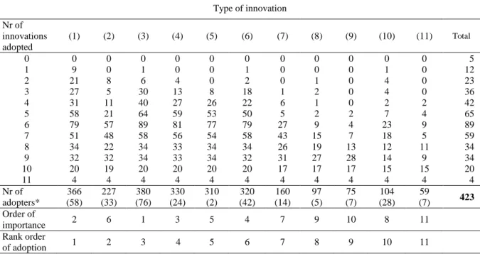
Since we have no precise way to estimate the relative profitability of each of the innovations available, no specific weights can be attached to them and we must rely on a simple counting of the innovations adopted by the sample households to measure the intensity of adoption. To the extent that all innovations can be adopted independently, the summing up operation appears legitimate. There emerges a systematic pattern of innovation adoption among rural producers of Cajamarca province. To see this, we have constructed a double-entry table (Table 2) in which each type of innovation as adopted in 2007 is related to the number of innovations adopted by each household. Innovation types are shown in the columns while frequencies are displayed in the rows. From cells (6,1) and (5,1), for example, we read that 79 households using innovation (1) in 2007 have adopted a total of 6 innovations, while 58 of them have adopted 5 innovations.

Table 2 contains several interesting pieces of information. First, we see that only 5 out of 423 households (1.18%) had not adopted any innovation at all in 2007 (as compared with a proportion of more than 60% in 2002). At the other end of the spectrum, only 4 households had adopted all the available innovations in 2007. The modal value of the number of innovations adopted is 6. Second, as indicated in the penultimate row, the most frequently adopted innovations are, by decreasing order of importance, innovations (3), (1), and (4). In particular, the twenty households which have adopted ten innovations out of eleven have all

chosen innovations (1), (3), (4), (5), and (6) while their adoption behaviour differs regarding the other innovations. Third, in the last row we have ranked the innovations by decreasing order of priority in adoption. To obtain their rank, we have looked at the most frequently adopted innovation when a household adopts successively one, two, three, and up to eleven innovations in total, taking into account all the innovations most frequently adopted in the previous rounds. Note carefully that we have numbered the innovations so as to reflect their ranking according to this last criterion. By construction, therefore, any figure located on the descending diagonal is greater than all the numbers that appear on its right and belong to the corresponding row. Roughly speaking (since we do not have precise data about costs of innovations), it is striking that innovations with higher adoption ranks are also those requiring cheaper inputs, which is a first clue pointing to the presence of a wealth constraint.

INSERT TABLE 2 ABOUT HERE

INSERT TABLE 3 ABOUT HERE

Overall, 2,427 innovations have been adopted, representing almost 6 innovations per household on an average, compared to less than one in 2002 (0.7). The rate of use of innovation potential (the aggregate number of innovations adopted by all sample households divided by the maximum number of adoptable innovations, that is, 11x423) was 52 percent in 2007, as against 6.3 percent in 2002. These summary statistics are presented in Table 3.

3.2 Econometric method

As we have previously pointed out, there are many reasons why new technology may fail to diffuse in rural areas of developing countries, and it is often difficult to disentangle their effects empirically. In this study, however, we naturally control for several important potential determinants of non-adoption of new technology. In particular, the sample households have all received basic information about the available innovations, the inputs involved are well distributed, and the way to use them well communicated by the promotores. Given imperfect credit (and insurance) markets, the liquidity constraint therefore suggests itself as a critical remaining determinant of differential rates of adoption. Note carefully, however, that insofar as the inputs associated with the new technologies must be paid upfront while the returns are uncertain, it is impossible to make out whether the wealth effect arises

from credit imperfections or from absent insurance. The liquidity constraint bites if, in the absence of credit, the potential adopter does not have funds prior to the realization of the gains from using the modern inputs associated with a new technology. But risk aversion is the problem if, in the absence of insurance, he is unwilling to borrow, or to use his own funds, to purchase the inputs required for the uncertain investment that a new technology represents (Foster and Rosenzweig, 2010).

In the following, we discuss the various measurement and estimation problems that stem from both the nature of our data and the context of the study.

To begin with, we measure the liquidity available to a household by its monetary income. Computed as the gross proceeds from the sale of milk and cheese on a per capita (and per annum) basis, this income is considered as a good proxy for the household savings that may be potentially used as working capital for the purpose of adopting innovations. Two distinct problems need to be addressed here. First, there is an obvious endogeneity between innovation adoption and income. To overcome it, we use an historical measure of income, i.e. the (gross) income of the household in 2002, as a proxy that is directly entered into the regression equation. A missing variable problem nevertheless remains and is the second challenge that we need to face. It can, indeed, be argued that there exists some unobserved heterogeneity in the form of individual characteristics of the agents that both determine their income, including past income, and their current innovation adoption behaviour. The effect of liquidity may thus be confounded with the influence of personal attributes such as willingness to innovate and skill level, which are plausibly correlated with income.

To minimize the risk of biased estimates caused by omitted variables, we follow a three-pronged strategy. The first plank of this strategy relies on three indicators of the innovativeness, skills, and entrepreneurial predisposition of the household heads that we are able to measure in our sample. These are: the number of innovations used in 2002, the average productivity of the cowherd in the same year, and the household’s willingness to acquire additional information about the innovations on offer. Let us discuss each of these control variables in turn.

Regarding the first of them, the absence of correlation between initial innovation adoption and wealth or income measures needs to be emphasized: for example, the average monetary income per head of adopter households (701 soles) was quite similar to that of non-adopter

households (685 soles) in 2002, the initial year.6 This apparently puzzling observation is not surprising since it is actually the result of a particular feature of our data. As a matter of fact, most innovations used in 2002 were cheap. Careful examination of data thus reveals that 83% of innovation adopters in 2002 had adopted less than three innovations and the two most frequently adopted innovations −double cow milking and multiple ploughing− have the special characteristics of being relatively time-consuming and toilsome, yet do not necessitate the purchase of modern inputs.7 As a consequence, adoption of innovations in the initial year should not be subject to the liquidity constraint, which removes the suspicion that it might be endogenous to initial household monetary income. Interestingly, while there is no correlation between initial wealth and innovation behaviour in 2002 (the correlation coefficient is equal to 0.04), the correlation between initial wealth and the number of innovations adopted in 2007 is significant with a coefficient of 0.27. This change is to be related to the fact that costly innovations have been adopted in significant numbers during the period 2002-2007.

Our second control variable, average cow productivity, is measured by the number of litres produced per cow per day, on an average for the whole year. Like the first variable, it is not well correlated with income and asset variables, and can therefore be treated as a measure of innovativeness that is largely independent of the household’s wealth status: for the year 2002, the correlation of average cow productivity with monetary income is 16%, with cowherd 18%, with grazing area 2%, and with improved pasture area close to 0%.8 Average cow productivity plausibly depends on the quality of grazing lands which varies from community to community (owing, in particular, to variations in altitude). In order to be able to interpret average cow productivity as a measure of skill or innovativeness of the household head, it will therefore be important to estimate our innovation adoption model with community fixed effects.

The third control variable is the rate of attendance of the household head to special information and training sessions organized by SP during the years 2002-2007 (see supra). We use a count variable, which takes on values between zero and five, since a maximum number of five special sessions have been accessible in the surveyed region. Note that as many as 69 percent of the sample households (292 out of 423) have chosen not to attend any

6

The same conclusion obtains if we compare the number of innovations adopted in 2002 with the following asset measures: grazing land area owned in 2002 by the household, the number of cows per head owned, and the type of irrigation used in the household farm.

7

Note that these two innovations are, respectively, the second- and third-most quickly adopted innovations when the whole period is considered (they are numbered (2) and (3) in Table 2).

8

It is therefore difficult to argue that households which enjoyed comparatively high cow productivity in the initial year benefited from scale economies.

of these special sessions. It is again striking that this variable is not well correlated with initial income: the correlation coefficient is equal to 0.11. It can nevertheless be argued that innovation adoption and the decision to attend training sessions are simultaneously determined. Or, the training decision is an outcome rather than a causal variable: herders first decide whether to innovate and, conditional on that decision, whether to attend training sessions. Although evidence provided at the end of this section does not support it such alternative scenarios - there are people who attend training events and do not later adopt innovations- we will check whether the effect of liquidity is modified when the training variable is removed from the regression equation. This naturally takes us to the next component of our estimation strategy.

Through the second approach, we want to verify that there is no omitted variable that explains at once the effects of all relevant variables, including the key variable of interest (wealth or income, our proxy for liquidity). Indeed, if wealth or income is obviously correlated with observables of the determinants of innovation adoption, it is plausible that it is also correlated with unobserved determinants. We will use a stepwise procedure starting from a simple regression of wealth on change in innovations adopted (controlling for the number of innovations adopted in 2002), and then adding controls successively. The variables measuring the household’s predisposition to innovate are entered first, followed by other household-level determinants and location-specific variables. We hope to show that the coefficient of the wealth variable is stable across these different specifications so as to reinforce our case for causality from wealth to innovation adoption.

The third and last plank of our estimation strategy consists of exploiting the exogenous difference between costly and costless innovations. In conformity with the above-noted absence of correlation between initial income/wealth and initial number of innovations adopted, we expect income to constrain innovation adoption only if innovations are costly, that is, only if they require the purchase of modern inputs. If this differentiated prediction could be borne out by the data, it would be difficult to believe that the effect of the liquidity constraint is spurious. Indeed, if the omitted variable problem exists, the way it affects the relationship between innovation adoption behaviour and initial income should not vary with the monetary cost of innovations.

The dependent variable that we use is the number of additional innovations adopted by the household during the period 2002-2007, controlling for the number of innovations used in the initial period. The former variable is denoted by Δinnovationsij, and the latter by innov_02ij,

our basic model, Δinnovationsij therefore appears on the LHS whereas innov_02ij and

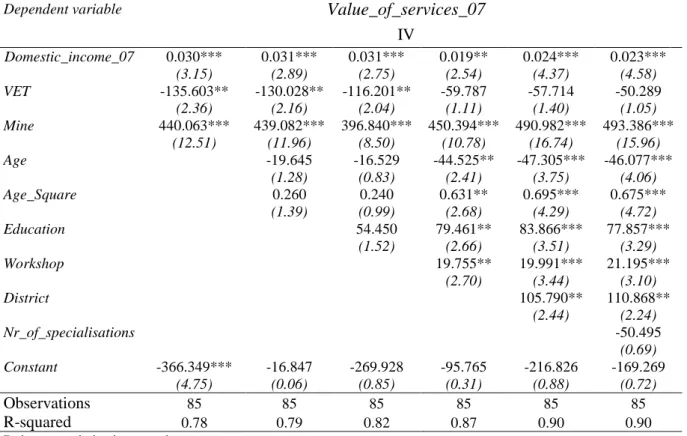
income_head_02ij, the initial monetary income of the household measured on a per capita basis, appear on the RHS.9 Moreover, we will test for a form that is quadratic in initial income because a concavity in the relation is strongly suggested by a semi-parametric fit (using Yatchew, 1958) of the relationship between innovation adoption and initial income (see Figure 1).

INSERT FIGURE 1 ABOUT HERE

Since the dependent variable of our model is a count variable, the innovation adoption equation is best estimated using a Poisson or a Negative Binomial Regression (NBR). As a robustness check, we have also estimated a simple OLS model the results of which are reported in the Appendix. Although somewhat less sharp, the OLS results essentially confirm the results obtained with the NBR. The NBR model to be estimated is:

The list of our independent variables includes three matrices, Zinnov, X, and G, and the error term, εij, is specific to the household. Standard errors are clustered at the community

level. The first matrix, Zinnov, consists of the aforementioned variables measuring the household’s innovative or entrepreneurial spirit and initial skill level: innov_02ij,

cow_productivity_02ij, another continuous variable, and training, a qualitative variable.

The matrix X comprises other household-level controls, more precisely physical assets privately owned by the household in the initial year: the grazing land area (labelled

grazing_area_02) and the size of its cowherd measured on a per capita basis (cowherd_02).

Since all innovations on offer are divisible, we do not expect that scale economies are present. On the other hand, if local land markets are quite inactive, the same is not true of the market for cows, and we may suspect that the number of animals owned by a household also measures its ability to obtain liquidity in case the need arises (hence our definition of this

9

We use the income per head instead of the aggregate income of the household because we believe that it is a better proxy of the liquidity constraint. If a household has a higher income than another, but has more dependents to cater to, it may actually be more liquidity-constrained. We may alternatively use both household income and household size as right-hand side variables, yet this does not essentially modify our results.

asset variable on a capita basis). Its impact on innovation adoption is therefore predicted to be positive, especially when used as an alternative to monetary income.

In X, we also include binary variables representing the type of irrigation system to which the household had access in the initial year. Since four irrigation systems are observed in our study area −natural irrigation, water conveyed by a central canal, access to a secondary channel infrastructure, and irrigation through sprinkling−, three dummy variables are used as regressors (denoted by irrigation_1, irrigation_2, and irrigation_3).

It must be noted at this stage that the interpretation of the coefficient of the liquidity variable is apparently difficult owing to the absence of any information about the educational level of the household head in our dataset. As a matter of fact, wealth or income may be significantly correlated with education, so that a positive income effect may represent a relationship between education and adoption (Foster and Rosenzweig, 2010). As will be explained later, however, our data about technical innovations provide us with an indirect test of the possible role of education. Another problem that may potentially plague our interpretation of initial income as a proxy measure of the liquidity or saving available to the household arises from the possible presence of land-related technical constraints that bear upon the profitability of innovations. This problem will be addressed when we discuss our results.

Unfortunately, we do not have information about personal characteristics of the household head such as age and education. We do not however believe that the latter, in particular, is a critical determinant of innovation adoption. This is because education levels are typically low and homogeneous in the study area. In fact, only the promotores have reached the secondary school and beyond.

Finally, the matrix G stands for location-specific variables. Toward that purpose, we use a binary variable that indicates the presence or absence of Nestlé multinational in the community to which the household belongs.10 This milk purchasing company directly operates in a number of the surveyed communities (in 8 out of 27 of them) and, since such a presence has the expected effect of reducing transaction costs, it is presumed to stimulate innovation adoption. Revealingly, the average milk purchase price obtained by local producers is higher in communities serviced by the Nestlé company than in the other communities, yet the difference is particularly noticeable during the rainy season. In point of

10

In fact, there is a smaller company, called Gloria, which also operates in the area. However, since all the villages in which it operates are also serviced by Nestlé, we will ignore it when we speak about the impact of a milk-purchasing company. We just have to bear in mind that our dummy is equal to one when either Nestlé or Gloria is present in the community (instead of Nestlé alone).

fact, prices are much more stable across seasons in the former than in the latter communities.11 In an alternative specification of the NBR, we drop the dummy Nestlé (equal to one if the community to which the household belongs is serviced by the company) and introduce fixed effects to control for the influence of community-specific characteristics. The latter model has the advantage of avoiding the problem of the possible endogeneity of Nestlé (the company has chosen its areas of operation on the basis of the local residents’ personal attributes)12 and, moreover, it allows to control for all characteristics of the promotores’ activities that possibly vary from community to community (number of operating promotores, intensity of their activities, etc.).

In conformity with the above-explained estimation strategy, we present different sets of results depending upon whether we introduce all the independent variables at once or using a stepwise procedure, and depending upon whether and how we exploit the difference between costly and cheap innovations. As already pointed out, we have chosen to display and fully discuss the estimates obtained by using the NBR model only. Moreover, we focus attention on the regression estimates with community fixed effects although we also comment on regressions that feature the Nestlé variable.

The descriptive statistics for the above variables as well as all other variables used in this study are reported in Appendix 1.

11

The average milk prices (in soles per litre of milk) are given in the table below from which it is apparent that prices in communities serviced by Nestlé are not only higher but also much more stable across the two seasons.

Nestlé absent Nestlé present

Dry season Rainy season Dry season Rainy season

2002 0.322 0.277 0.358 0.357

2007 0.423 0.369 0.486 0.477

12

Endogeneity is quite unlikely, though, since it assumes that company managers have a good knowledge of the personal qualities of rural producers in different locations. Moreover, it is noteworthy that its areas of operation have not changed during the period under review and that they had been initially chosen because of their comparatively easy accessibility.

3.3 First set of results

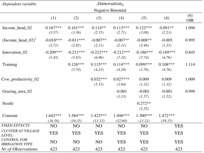
In Table 4, we present the results of our estimation of the innovation adoption equation in a stepwise manner. Column (1) reports the estimates obtained when only the initial income (and its square value) and the initial number of innovations adopted are entered as regressors. Then, in the following columns we have successively added the two remaining components of

Zinnov, −the measure of training and initial cow productivity−, the variables representing the

irrigation system, the pasture land area, and the Nestlé dummy. The variable cowherd is omitted for reasons explained below.

INSERT TABLE 4 ABOUT HERE

The central result is the strong and robust presence of a liquidity constraint. When we run the stepwise regression model, it selects the initial income (and its square term) and the initial stock of innovations as the only independent variables. The coefficients of the two income terms are strongly significant statistically (at the 99 percent confidence level), and their signs confirm the concave shape of the innovation adoption function. When we add successively

training, cow_productivity_2002, grazing_area_02, the irrigation dummies, and Nestlé, this

relationship continues to hold despite the fact that training, cow_productivity_02, and Nestlé are all significant at 99% level.

As expected, the size of the (positive) coefficient of income_head_02 diminishes between the first and last regressions, yet the fall (by about one-fourth of its initial value) is almost entirely due to the introduction of initial cow productivity as a control. A plausible explanation is that this variable captures community fixed effects in the form of variations in the quality of pasture land between villages. This interpretation seems to be confirmed when we re-estimate the complete model with community fixed effects and without Nestlé. It then appears that the coefficient of cow_productivity_02 is no more significant, suggesting a strong redundancy of fixed effects (see column (6)). It is still justified to keep that variable in the regression because it potentially capture within-community variations of land quality as well as variations in household dynamism.13 It is noteworthy that in the regression with community fixed effects the square income term is no more significant.

13

Revealingly, when cow_productivity_02 is dropped from the regression with fixed effects, the coefficient of income_02 increases significantly.

On the contrary, the cowherd_02 variable has been dropped because it does not add any explanatory power to the innovation adoption equation. Its coefficient is not significant and its presence does not modify the other effects, including that of initial income, whether we look at the significance or the size of the corresponding coefficients. This is not surprising since the correlation between cowherd_02 and income_head_02 is quite high (equal to 0.593).

As has been stressed earlier, it is impossible to disentangle the effects of credit constraints and absent insurance. The data available do not allow us to determine whether the liquidity constraint arises from credit imperfections or from greater risk aversion and smaller protection from risk among poorer producers. From Section 4, we will learn that the usual practice is for innovation suppliers to grant credit to adopters, yet default is not infrequent so that suppliers have learned to screen their customers. There are therefore two possible stories behind our central result. On the one hand, poor households may be reluctant to accept credit with a view to adopting innovations associated with modern inputs because they have doubts about their ability to repay the loans due to uncertainty of returns or other reasons. On the other hand, innovation suppliers may refuse to grant loans to poor households because they think reimbursement is too uncertain.

Regarding the remaining effects, the coefficients that are significantly different from zero have the expected sign. Thus, the initial number of innovations influences adoption negatively and significantly (99% confidence level). Even though it reflects the household’s willingness to innovate, a larger initial stock of innovations leads to a smaller absolute increase in the subsequent period: this is the mechanical consequence of the existence of a ceiling on the total number of adoptable innovations. Second, the frequency of attendance to special information and training sessions is positively related to innovation adoption. The fact that the addition of

training does not affect the relationship between Δinnovationsij and income_head_02 is good news since, as pointed out earlier, training can be suspected of reverse causality. Third, communities directly serviced by Nestlé, which tend to benefit from higher milk purchase prices (see above), appear to have adopted more additional innovations than other communities during the years 2002-2007.

3.4 Second set of results

We now consider the results obtained when the third approach to testing the effect of a liquidity constraint is followed. Because we possess rather detailed information about the available technical innovations and their varying characteristics in terms of working capital

requirements, we can re-estimate the innovation adoption equation by isolating innovations that require labour efforts and know-how, but no modern inputs, for effective use. Another advantage in separating innovations that incorporate costly inputs from the others is the following. If education, an omitted variable plausibly correlated with wealth or income, influences technology adoption positively, we expect the income-adoption relationship to hold for both categories of innovations unless we believe that costly innovations are necessarily more sophisticated or skill-intensive (a possibility that we will put under scrutiny).

The techniques that fit the above definition of cheap innovations happen to be the first five innovations listed in Table 2: hygienic measures in milking operations, double cow milking, multiple ploughing, application of organic fertilizers, and the use of lime to improve productivity of grazing fields. Costly innovations correspond to the other six innovations, numbered (6) to (11). We label these two categories of innovations Δcheap_innovations (the number of additional innovations of the cheap kind adopted by the household during the 2002-2007 period), and Δcostly_innovations (the number of additional costly innovations adopted). Our sample data show that 94 out of 423 households (22 percent) have not adopted any costly innovation during the period under concern.

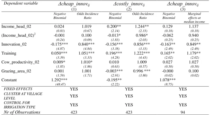
In the first two columns of Table 5, we report the separate estimates for the full model when innovations are partitioned in the above way and the complete sample is used. (For the sake of brevity, we show only the results for the regressions with community fixed effects, yet the results obtained with the alternative specification featuring the Nestlé dummy are quite similar). The estimated coefficients of income_head_02 are strikingly different once we distinguish between the two types of innovations: while for costly innovations the value of the coefficient is about 0.20 and is significant (at 95 percent level), it is equal to only 0.02 for cheap innovations, which is not statistically different from zero. Note that the results obtained for each regression are confirmed at every step of the stepwise estimation procedure (results not shown). As for the coefficient of the square income term, it is negative (-0.013) and significant for costly innovations while it is very low and insignificant for cheap innovations.

INSERT TABLE 5 ABOUT HERE

In addition to initial monetary income, the initial number of innovations adopted and participation in training sessions remain strong determinants of the adoption of additional costly innovations. It bears emphasis that the coefficient of training is four times as large for costly innovations (about 0.20) than for costless innovations (0.05), yet in the latter case the

effect remains also strongly significant. Moreover, the grazing area owned by the household is a strongly significant factor influencing the adoption of costly innovations, and its influence is negative. Upon closer look, it appears that the effect is largely attributable to a single innovation, i.e. improved seeds for grazing fields.14 This is the only costly innovation which is actually applied to the grazing land rather than to the animals. The implication seems to be that, by increasing land productivity through the use of improved seeds, households endowed with smaller land endowments substitute quality for quantity.

Finally, the (positive) coefficient of cowherd_02 is not significant. However, when we drop the initial income variables from the regression for costly innovations, we find that the coefficient of cowherd_02 becomes statistically significant, again without modifying the effects of the other independent variables (results not shown). This seems to indicate that

cowherd_02 is an alternative measure of household liquidity, yet less precise than initial

monetary income.15

The need to differentiate between costly and cheap innovations when assessing the impact of liquidity emerges clearly from Figure 2, which displays the results of two separate semi-parametric fits of the relationship between innovation adoption and initial (per capita) income. While the relation is unambiguously positive for costly innovations and actually replicates the relation obtained when all innovations are aggregated, the relation appears to be absent for cheap innovations.

INSERT FIGURE 2 ABOUT HERE

We must now reckon that it is not entirely satisfactory to estimate the determinants of the adoption of cheap innovations on the basis of the complete sample. This is because of the presence of households which have adopted both costly and cheap innovations. Another test of the presence of a liquidity constraint therefore consists, for cheap innovations, to restrict our attention to households which have adopted a varying number of cheap innovations to the exclusion of any costly innovation. As indicated above, there are 94 such households. When we re-estimate the cheap innovation adoption equation based on this restricted sample (see column (3)), we find again that, as expected, no income effect is at work (the z-value for the

income_head_02 coefficient is as low as 0.18). In addition, the stepwise procedure for cheap

14

Indeed, when we remove that innovation from the list of costly innovations and we re-run the regression, the coefficient of grazing_area comes close to losing its statistical significance.

15

When all innovations are aggregated, and we similarly drop the initial income variables from the regression, the coefficient of cowherd_02 does not become significant, but it is positive whereas it was negative in the presence of the income variables.

innovations reveals that the income effect is never statistically significant even when only the initial income variables and the initial number of innovations are used as explanatory variables.

Lastly, it must be noted that the coefficient of training remains significant when the sample size is reduced from 423 to 94 households. The persistence of the training effect in columns (1) to (3) means that specific skills need to be acquired for the effective use of both costly and cheap innovations. As pointed out above, however, the role of such skills is more important for the former than for the latter innovations.

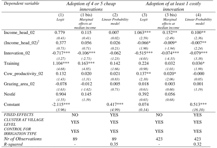
The differentiation between cheap and costly innovations can be exploited in still other ways to further test the robustness of our results. We can thus estimate a model in which the dependent variable is a dummy equal to one if the household has adopted four or five cheap innovations to the exclusion of any costly innovation, and to zero if it has adopted less than four cheap innovations. The sample used in this instance is restricted to 89 households. When this is done with the complete set of explanatory variables, either by using a logit model without community fixed effects but including Nestlé or with a simple linear probability model with these fixed effects, the result is neat: there is no income effect but the coefficients of innov_02 and training are strongly significant (see columns (1) and (2) in Table 6). Conversely, we can estimate another model in which the dependent variable is a dummy equal to one if the household has adopted at least one costly innovation and to zero otherwise. Here, we retain the full sample. Results shown in columns (3) and (4) of the same table reveal that the effect of initial income is then strongly significant, whether we use the logit or the OLS models.

INSERT TABLE 6 HERE

As an additional robustness check, we carry out the following exercise. Our benchmark comes from contrasted estimates for six costly and five cheap innovations (see columns (1) and (2) in Table 5). We then gradually broaden the category of costly innovations by adding, one by one, innovations subtracted from the cheap category. Cheap innovations are successively taken out of their original category by descending order of their presumed cost. More precisely, to the category of costly innovations we first add the application of lime (to reduce the acidity of grazing land), then the application of organic fertilizers, and lastly multiple ploughing. Table 7 compares the values of the coefficient of income_head_02 resulting from this stepwise estimation procedure, using the NBR model (first row) and the

OLS model (second row), both with community fixed effects. As expected, the value of this coefficient decreases monotonically as additional innovations of the cheap type are added to those of the costly type. On the other hand, the same coefficient estimated for the increasingly narrow category of cheap innovations always remains statistically non-significant.

INSERT TABLE 7 HERE

The non-significance of the initial income variable for cheap innovations, whichever way we define this category, suggests that the influence of income for costly innovations may not be reasonably traced to education. Could it be said, however, that cheap innovations correspond to rather simple techniques so that the role of education in facilitating the decoding of new information for their effective use is necessarily limited? The fact of the matter is that the relationship between the cost of innovations and their educational requirements is not straightforward. Thus, the most frequently adopted innovation, innovation (1) which consists of hygienic measures applied during milking operations, is clearly care-intensive, and the same is true of innovations (4) and (5), the application of organic fertilisers and lime, respectively, which also happen not to be among the costly innovations. It is true that certain innovations, most of them costly, require specific knowledge in addition to general education, yet the training variable takes that effect of acquired knowledge into account.

Another interpretation problem that deserves to be mentioned arises from the fact that a category of producers present the double characteristics of being comparatively poor and more strongly exposed to income variability. These are the producers of low quality cheese. We cannot therefore exclude the possibility of a confounding effect in the sense that that the impact of low incomes on innovation adoption could be attributable to risk rather than a pure liquidity problem. A simple way of testing this alternative explanation consists of adding as a regressor a binary variable which is equal to one when the household is a low quality cheese producer (it does not produce any fresh milk or high quality cheese, whether in the initial or in the terminal year), and to zero otherwise. We also add an interaction term between this dummy and initial (per capita) income. We find that the coefficients of these two variables are far from being significant whereas all our other results, in particular the positive impact of initial (per capita) income on innovation adoption, stand unchanged (results not shown). Our interpretation in terms of a liquidity or savings constraint therefore seems warranted.

The last exercise that we want to carry out obeys the need to better understand the way in which the training variable exerts its impact on innovation adoption. As a matter of fact, since we know that the liquidity constraint is present only for costly innovations, we expect that for this category of innovations the effect of training manifests itself only if the liquidity problem is surmounted. If it is not, participation in training activities cannot result in the adoption of costly innovations. We can test for this hypothesis in the following way. We estimate a censored Poisson model (since the liquidity constraint is operating) to explain adoption of costly innovations, and we include an interaction term between the initial income and training variables in the list of regressors. The predicted outcome is that the interaction effect is statistically significant (and positive) and causes the direct effect of training to vanish. The results, presented in Table 8, fully confirm the prediction. Incidentally, they provide evidence that the decision of participation in training sessions does not necessarily follow the adoption decision: people may have attended training events and find themselves later unable to adopt innovations due to the liquidity constraint. Note carefully that the effect of initial income remains strongly significant (the square term has been dropped because the relationship between initial income and adoption of costly innovations is close to linear, as shown in Figure 2). The conclusion is, therefore, that liquidity has a significant impact, and participation in training sessions encourages adoption of costly innovations provided that liquidity is not constraining. A look at the Odds Incidence Ratios reveals that the effect of initial income is quite important, especially when associated with participation in training sessions: if initial income per head is increased by 1,000 soles, the number of additional costly innovations adopted increases by 51 percent, but each training session adds a further increase of 166 percent (per unit of 1,000 soles) to that effect.

INSERT TABLE 8 HERE

4. The supply of extension services and the wealth constraint

4.1.Creation of a market for extension services and credit transactions

The “promotores” programme launched by SP in La Encanada and Hualgayoq districts was actually the outcome of a rethink of a previous scheme known as the “kamayoq” programme. Under the latter scheme, extension agents, duly elected by their village