HAL Id: hal-03207854
https://hal.archives-ouvertes.fr/hal-03207854
Submitted on 26 Apr 2021HAL is a multi-disciplinary open access archive for the deposit and dissemination of sci-entific research documents, whether they are pub-lished or not. The documents may come from teaching and research institutions in France or abroad, or from public or private research centers.
L’archive ouverte pluridisciplinaire HAL, est destinée au dépôt et à la diffusion de documents scientifiques de niveau recherche, publiés ou non, émanant des établissements d’enseignement et de recherche français ou étrangers, des laboratoires publics ou privés.
Tropical mangrove forests as a source of dissolved rare
earth elements and yttrium to the ocean
Duc Huy Dang, Zhirou Zhang, Wei Wang, Benjamin Oursel, Farid Juillot,
Cecile Dupouy, Hugues Lemonnier, Stephane Mounier
To cite this version:
Duc Huy Dang, Zhirou Zhang, Wei Wang, Benjamin Oursel, Farid Juillot, et al.. Tropical mangrove forests as a source of dissolved rare earth elements and yttrium to the ocean. Chemical Geology, Elsevier, 2021, pp.120278. �10.1016/j.chemgeo.2021.120278�. �hal-03207854�
2
Abstract: Rare earth elements (REEs) and Y are commonly used as geochemical proxies for
16
water chemistry, history of the continental crust and provenance studies. At the continent-ocean 17
interface, the estuarine geochemistry of REEs is commonly considered to be driven by a large-18
scale removal. Consequently, the river-borne flux of dissolved REEs to the marine budget is 19
assumed as a minor fraction. Here, we report a significant release of dissolved REEs, together 20
with a fractionation between light, heavy REEs and Y, in the tropical mangrove estuaries of New 21
Caledonia. These observations were associated with internal recycling within the redox-dynamic 22
mangrove system. The possible contribution of groundwater can be ruled out based on water 23
stable isotopes. These findings imply that tropical mangrove estuaries act as a sizeable source of 24
REEs and Y to the ocean rather than as a buffer zone. We extrapolated our data toward global 25
dissolved fluxes of REEs and Y through the mangroves. This preliminary calculation suggests 26
that the mangrove system supplies 2.6-5% of global river-borne dissolved Nd, a REE with the 27
most comprehensive mass balance. Therefore, oceanic mass balance budget models may need to 28
consider this atypical system as an input to balance the global distribution of REEs and Y. 29
Keywords: Rare earth elements, yttrium, water stable isotopes, mangrove, estuary.
3
Introduction
31
Over the past decade, rare earth elements (REEs or the lanthanide series), Y and REE isotopes 32
have received significant attention in geochemistry as tracers of the geological history of the 33
continental crust and provenance study (Bayon et al., 2015). In paleoenvironmental studies, REEs 34
are also commonly used as proxies to reconstruct water chemistry and oxygen saturation as per 35
the distinct behaviour of Ce during redox transitions (Auer et al., 2017; Wallace et al., 2017). The 36
fractionation between the light REEs (LREEs), heavy REEs (HREEs) and the non-lanthanide Y 37
can also highlight the mechanisms of particle transport, sediment deposition and even geological 38
features (e.g., iron formation) over the Earth’s history (Bayon et al., 2015; Planavsky et al., 39
2010). More recently, because of the implication of REEs in novel technologies, REE anomalies 40
(increased in concentrations of a specific REE relative to its neighbouring REEs) could also be 41
used as a proxy for emission sources (Dang and Zhang, 2021; Ma et al., 2019; Tepe et al., 2014). 42
However, the environmental chemistry of REEs remains fragmented, mostly regarding their 43
anomalous behaviour across the river-estuarine-coastal water mixing zone where the 44
fractionation between LREEs and HREEs is often associated with the redistribution of REEs 45
among the dissolved and particulate fractions and the formation of stable dissolved complexes 46
(Nozaki et al., 2000; Sholkovitz and Szymczak, 2000; Sholkovitz, 1995). As a consequence, the 47
ocean mass budget of REEs remains unbalanced with missing fluxes at the global scale (Arsouze 48
et al., 2009; Garcia-Solsona and Jeandel, 2020; Pourret and Tuduri, 2017; Tachikawa et al., 49
2003). 50
The interpretation of estuarine REE behaviour is fundamental to highlight their geochemistry at 51
the continent-ocean interface. One conventional feature derived from decades of investigation on 52
REEs’ estuarine geochemistry is that large-scale removal of dissolved REEs (especially LREEs) 53
occurs in the estuarine mixing zone (Elderfield and Greaves, 1982; Lawrence and Kamber, 2006; 54
Nozaki et al., 2000; Pourret and Tuduri, 2017; Sholkovitz, 1995). This phenomenon minimizes 55
the effective continental flux of REEs to the ocean and subsequently affects the marine budget 56
calculations of REEs (Nozaki et al., 2000). Various factors would lead to such extensive removal 57
of REEs. These include planktonic uptake, coprecipitation with ferromanganese oxyhydroxides 58
and salt-induced coagulation of colloids (Hoyle et al., 1983; Nozaki et al., 2000; Sholkovitz and 59
Szymczak, 2000). However, a limited number of publications pointed out a supply of dissolved 60
4 REEs in the mid-estuary zones (Lawrence and Kamber, 2006; Nozaki et al., 2000). This REE 61
release could be associated with desorption from terrigenous suspended particles or 62
remineralization in the estuarine system. 63
Moreover, most of the estuarine systems investigated so far for REEs geochemistry were major 64
well-oxygenated riverine systems. However, it has been demonstrated that REEs cycling in 65
marine waters can be impacted by redox variations (Bau et al., 1997). This process is particularly 66
important as it can increase the effective continental REE flux to the oceans through enhanced 67
supply to the water column upon dissolution of REEs-bearing oxyhydroxide phases. Therefore, 68
further insights on REE behaviour across the redox-sensitive estuarine mixing zone are needed to 69
strengthen our understanding of the REE geochemistry at the continent-ocean interface. 70
Tropical mangrove forests are of great interest to investigate these environmental conditions. 71
First, they cover a large surface area (150,000 km2) where complex hydrological processes 72
balance abundant precipitation, surface runoff, and evaporation (Spalding, 2010). Moreover, the 73
combination of elevated and annually constant temperature patterns with high bioavailability of 74
natural organic matter boosts bacterial respiration, promoting hypoxia (Dubuc et al., 2019). To 75
date, very limited studies on REEs focused on this critical ecosystem as it is generally assumed 76
that the mangrove systems act as a buffer zone retaining trace elements and thus contribute a 77
minor input for REEs to the oceans (Marchand et al., 2012). 78
Here, we investigated REE internal cycling within two estuarine mangrove systems in the 79
subtropical region of New Caledonia. We meticulously measured dissolved REEs and Y over a 80
24-hour cycle in mangrove stations during a dry season and the spatial variations across the 81
estuary in a rain season. To track whether additional water masses alter the mixing between the 82
fresh and seawater endmembers, we also measured stable water isotopes (δ18O and δD) to assess
83
the hydrologic regime. We compared the stable water isotopes in these mangrove systems with 84
other river waters collected in southeastern New Caledonia to verify the signature of the 85
freshwater endmembers. Altogether, the data highlights REE behaviour during the estuarine 86
mixing and document the mangrove forest's role on REE cycling at the continent-ocean interface. 87
This dataset will help answer whether the REE continental flux from the tropical mangrove-88
dominated estuaries should be included in the REE marine budget. 89
5
Materials and Methods
90
Study site description
91
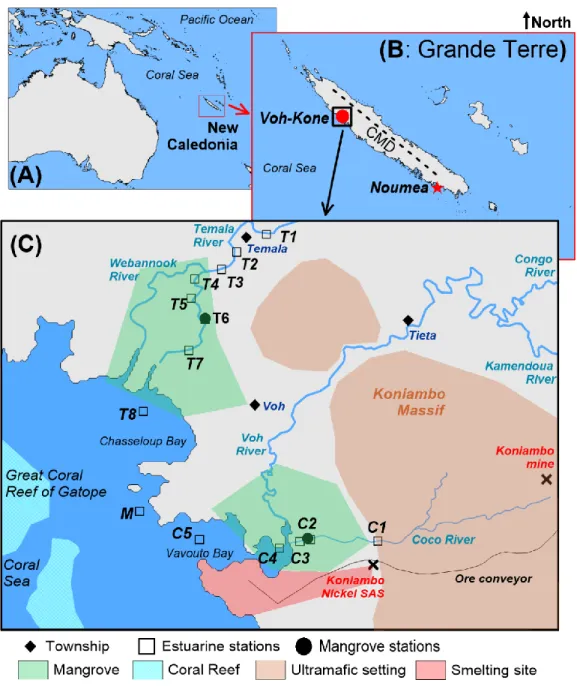
In the Southwest Pacific Ocean, New Caledonia is surrounded by the Coral Sea (Figure 1A,B). 92
The main island “Grande Terre” is 400 km long and 64 km wide with a semi-arid tropical climate 93
along the west coast. The whole island is also bordered by a coral reef enclosing a lagoon of over 94
20,000 km2. The rich reef diversity and associated ecosystems were inscribed as a UNESCO 95
World Heritage Site in 2008. On the other hand, most of the island is mountainous with vast 96
ultramafic masses, schists and outcrops of basalt (Lillie and Brothers, 1970). Weathering of the 97
ultramafic rocks’ surface led to the formation of thick lateritic regoliths (tens of meters) hosting 98
deposits of transition metallic elements of prime economic importance (Dublet et al., 2014; Noël 99
et al., 2014). Between the lucrative mineral-rich land and the sea of tremendous ecological 100
importance, the mangrove system acts as a buffer zone to filter heavy metals from reaching the 101
reef (Marchand et al., 2012). 102
The hydrological behaviour of the Grande Terre is clearly distinct between the southwestern and 103
northeastern coasts because of the ‘rain-shadow’ effect across the central massif divide (Terry 104
and Wotling, 2011) (Figure 1B). Accordingly, the southwestern coast (leeward) tends to be drier 105
than the windward northeastern coast. Overall, the hydrologic regime is characterized by high 106
annual variability of rainfall amount and extreme events. Moreover, high and steep watersheds 107
are associated with flash floods and thus rapid water transfer to the lagoons (Desclaux et al., 108
2018). 109
The Voh-Kone region (Northwest of the Grande Terre, Figure 1B) is an area of great economic 110
and ecological interest. The Koniambo Massif hosts a large mine (Koniambo mine, Figure 1C), 111
one of the largest nickel reserves in New Caledonia. The ore is conveyed to a coastal smelting 112
site (Koniambo Nickel SAS, Figure 1C). Besides, the hydrologic system mainly comprises of 113
two major rivers (Temala and Voh) discharging into the mangroves, then the bays of Chasseloup 114
and Vavouto, respectively. Moreover, the hydrologic system comprises also of relatively smaller 115
streams, such as the Coco River. These small tributaries have their flows significantly reduced 116
during the dry season. 117
6 This study focused on the Temala and Coco Rivers (Figure 1C) in the Voh region. The Temala 118
River originates from outside of the Koniambo Massif and discharges into Chasseloup Bay. It is, 119
therefore, considered not impacted by mining activities. On the other hand, the Coco River’s 120
sources are in the Koniambo Massif hosting the Koniambo Mine. Along its course toward 121
Vavouto Bay, the Coco River meanders parallelly to the ore conveyor. The Koniambo Nickel 122
SAS smelting site is indeed only ca. 1.2 km away from the stream (Figure 1 C). Therefore, it is 123
highly probable that this river is subject to anthropogenic impacts. Besides this contrasted 124
exposition to anthropogenic sources, the natural geological settings of both rivers also differ. The 125
Temala River catchement is made of soils developed on volcano-sedimentary rocks (cherts, 126
basalts), whereas the Coco River catchment is composed of Ni-laterites developed on ultramafic 127
rocks (peridotites) (Merrot et al., 2019). 128
We also investigated river waters (Dumbea, Coulee, Tontouta, Pirogue, Table 1) around Noumea 129
in the Grande Terre's Southeast (Figure 1B) as a reference site for hydrological assessment using 130
salinity and water isotope mixing. 131
Water sampling
132
We organized multiple sampling trips to investigate the hydrologic regime and REE cycling. The 133
two first sampling campaigns were organized in June 2019 (dry season) and March 2020 (rain 134
season) to collect samples in the Voh-Kone region (Temala and Coco Rivers). We also collected 135
samples in four southeastern rivers (Dumbea, Coulee, Tontouta, Pirogue) in January, March, 136
October and November of 2018. The March samples were collected during and after the Hola 137
tropical cyclone while other samples are collected during the dry season. 138
During a dry season (June 2019), the first campaign aimed for a high-temporal resolution 139
sampling in the mangrove forests (sites C2 and T6, hereafter referred to as “mangrove stations”, 140
Figure 1C). For that purpose, two automatic samplers (ISCO) were deployed during high tide
(8-141
9h AM). The samplers were programmed to collect water samples one hour after installation to 142
ensure the resettlement of resuspended sediments during deployment. The first water samples 143
were collected at 9h AM at C2, and 10h AM at T6. Following samples were collected every hour. 144
At the end of the 24-hour automatic sampling cycle, all samples were filtered (0.22 µm, cellulose 145
acetate, Sartorius) directly on site. The filtered waters for stable water isotopes were filled to the 146
7 top to avoid water-air exchange, while samples for elemental analysis were acidified to pH<2 147
with ultra-trace HNO3 (Merck). The samples were then immediately shipped by air to Trent
148
University for analysis. 149
In 2020, during the rain season, a series of samples were collected across the salinity gradient 150
along the Temala (T1-T8) and Coco (C1-C5) rivers (hereafter referred to as the “estuarine 151
stations”, Figure 1C). An additional sample was collected in the lagoon to serve as a marine 152
endmember (M, Figure 1C). The samples were treated with the same protocol as in 2019 before 153
being shipped to Trent University. 154
All the filters, sampling and storing bottles were previously rinsed with 10% HCl and milli-Q 155
water (18 MΩ cm) in the laboratory and with river or lagoon water in the field. 156
Water stable isotopes
157
Water stable isotopes (δ18O and δD, deuterium) were measured using a Liquid Water Isotope
158
Analyzer (LWIA-24d, Los Gatos Research) at the Water Quality Center (Trent University, 159
Ontario, Canada). The delta notation was calculated relative to the V-SMOW (Vienna-Standard 160
Mean Ocean Water) standard. 161 𝛿18𝑂 = ( (18𝑂 𝑂 16 ) 𝑠𝑎𝑚𝑝𝑙𝑒 (18𝑂 𝑂 16 ) 𝑉−𝑆𝑀𝑂𝑊 − 1 ) × 1000(𝐸𝑞. 1) 162 𝛿𝐷 = ( ( 𝐷 𝐻 1 ) 𝑠𝑎𝑚𝑝𝑙𝑒 ( 𝐷 𝐻 1 ) 𝑉−𝑆𝑀𝑂𝑊 − 1 ) × 1000(𝐸𝑞. 2) 163
Analytical recovery was assessed using two isotopic natural water reference materials (CRMs, 164
Elemental Microanalysis, UK), covering the range of δ values found in natural waters (Table 165
S1). Averages and standard deviations of each measurement (standards and samples) were
166
calculated based on eight injections (i.e., n = 8, 750 nL each). We also used ultra-high purity 167
water (18.2 MΩ cm) as an in-house standard to bracket every two samples to monitor analytical 168
8 drift and eliminate any memory effects. However, no correction was necessary. Analytical
169
recovery of stable water isotopes is reported in Table S1. 170
Elemental analysis
171
To accurately determine the concentrations of REEs and Y at the ng/L levels in complex 172
environmental matrices (seawater), we have performed a preconcentration step using column 173
chromatography before analysis by Inductively Coupled Plasma Mass Spectrometry (ICP-MS). A 174
full description of the REE column chromatography and ICP-MS analysis were reported 175
elsewhere (Dang and Zhang, 2021; Ma et al., 2019). Briefly, REEs and Y in the filtered water 176
samples were preconcentrated using 0.2 mL Nobias Chelate-PA1 resin (Hitachi High-177
Technologies). An aliquot of 50 mL of samples buffered at pH 6 was loaded on previously 178
washed and conditioned resin. The seawater matrix was then washed off with 40 mL 0.05 M 179
acetate buffer solution (pH = 6). REEs and Y were collected by eluting 20 mL of a 1 M HNO3
180
solution through the column. This aliquot was collected into a 30 mL PTFE vessel and 181
completely evaporated on a hotplate at 100oC. A final 2 mL of 0.5 M HNO3 was added to retake
182
the REEs and Y. 183
All acids used to clean and wash the resins were double-distilled trace metal grade. The acetate 184
buffer was also passed through the Nobias column for purification. We also meticulously 185
checked procedural blanks and column recovery in every batch of 10 samples. Procedural blanks 186
were between 0.1 to 29 pg of REEs and Y and significantly less than their mass in natural 187
samples. Several aliquots (50 mL) of certified reference seawater CASS-6 (National Research 188
Council of Canada, NRCC) were also repeated to test column recovery (Ma et al., 2019). 189
REEs and Y were determined using a triple quadrupole ICP-MS (8800 Agilent Technologies) at 190
the Trent Water Quality Center. All REEs and Y were analyzed in MS/MS mode with O2 as the
191
reaction cell gas. Detection limits were in the range of 0.1-0.4 ng/L. Although there were no 192
certified reference materials for REEs, we compared the REEs and Y concentrations measured in 193
an NRCC natural water certified reference material (SLRS-6) to the values reported in a 194
European interlaboratory calibration (Yeghicheyan et al., 2019). Excellent recovery was 195
observed; the detailed data are reported in Table S2. 196
Normalization of REE patterns and calculations of anomalies
9 A common practice in the scientific community to eliminate the Oddo-Harkins effect and
198
compare samples is to normalize the measured REE concentrations to geological materials (e.g., 199
upper continental crust, shales, chondrite) or offshore seawater (Piper and Bau, 2013). Here, we 200
normalized the measured concentrations of dissolved REEs to Post-Archean Australian Shale 201
(PAAS (McLennan, 2001)) (Goldstein and Jacobsen, 1988; Ma et al., 2019; Piper and Bau, 202
2013). The shale-normalized concentrations are hereafter referred to as REEPAAS.
203
In the current literature, excess or depletion of an REE relative to its neighbouring REEs are 204
referred to as positive or negative anomaly of this element (REE/REE*). Accordingly, the REE 205
anomalies could be determined by several approaches (e.g., arithmetic mean, geometric 206
extrapolations, modelling the shape of PAAS-normalized patterns, third-order polynomial fit). 207
Using all these approaches, Hatje et al. have demonstrated minor variability in the final results 208
(Hatje et al., 2016). Therefore, we calculated Ce, Eu, and Gd anomalies using the following 209
equations (arithmetic mean). 210 𝐶𝑒 𝐶𝑒⁄ = 2 × 𝐶𝑒𝑃𝐴𝐴𝑆 𝐿𝑎𝑃𝐴𝐴𝑆+ 𝑃𝑟𝑃𝐴𝐴𝑆(𝐸𝑞. 3) 211 𝐸𝑢 𝐸𝑢⁄ = 2 × 𝐸𝑢𝑃𝐴𝐴𝑆 𝑁𝑑𝑃𝐴𝐴𝑆+ 𝑆𝑚𝑃𝐴𝐴𝑆(𝐸𝑞. 4) 212 𝐶𝑒 𝐶𝑒⁄ = 𝐺𝑑𝑃𝐴𝐴𝑆 0.33 × 𝑆𝑚𝑃𝐴𝐴𝑆+ 0.67 × 𝑇𝑏𝑃𝐴𝐴𝑆(𝐸𝑞. 5) 213
Results and Discussions
214
Physical-chemical properties
215
At both mangrove stations (C2 and T6, Figure 1B), pH values varied within a narrow range (7.8 216
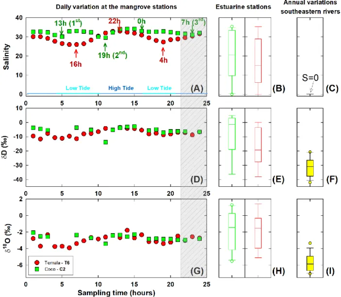
± 0.1, n = 48, Table 1 and Figure S1B). Besides, the daily variations in salinity followed a 217
sinusoidal curve, typical of estuarine systems (Figure 2A). This variation pattern is more 218
noticeable at Temala with low tide (S = 26) recorded at 4h and 16h, and high tide (S = 33) at 22h. 219
However, the salinity pattern at Coco is significantly distinct, with two events marked by steep 220
drops at 13h, 19h and a third gradual decrease from midnight until 7h AM (1st, 2nd, 3rd as marked 221
in Figure 2A). The variation range of salinity in Coco is also narrower (29.6 to 34.2) than in 222
Temala (26.0 to 33.0) (Table 1). 223
10 Temperature variations also help distinguish the two systems. Water temperatures increased from 224
16.8oC at 11h and held constant at ca. 17.5oC at Temala (Figure S1A, average of 17.3 ± 0.2oC, n
225
= 24, Table 1). However, the temperature pattern at Coco showed broader variations (15.5oC to 226
16.5oC, average of 16.1 ± 0.3oC, n = 24, Table 1) with temperature drops at 11h and 21h (Figure 227
S1A). Minimums in water temperatures at Coco are lagged by two hours relative to the salinity
228
minimums (13h and 19h, Figure 2A). 229
Across the entire estuaries (estuarine stations), salinities ranged from 0 to 34.9 for the river water 230
and marine endmembers, respectively (Figure 2B). On the other hand, all the river samples 231
collected from the Southeast of New Caledonia are freshwater with a salinity of zero (Figure 232
2C).
233
Stable water isotopes and the hydrologic regime
234
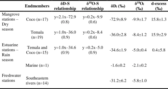
The δD and δ18O pairing. As the mangrove stations have narrow daily salinity variations (Table
235
1), so too is the range of stable water isotope compositions relative to the whole estuaries (Figure
236
2 D-I). At the mangrove stations, the δD-δ18O relationship has the equation of δD = 4.3 × δ18O + 237
5.5 (n=40, Figure S2). The slope of 4.3 ± 0.6 is typically lower than other tropical Pacific regions 238
(5.1 to 6.5, Conroy et al. (2014)), and the global seawater average of 7.4 (Rohling, 2007). This 239
indicates a strong influence of the evaporation process in the mangrove during the dry season. 240
Across the estuaries, the δD-δ18O relationship of Coco and Temala waters aligns with
241
southeastern rivers with the equation of δD = 4.8 × δ18O - 4.6 (n=29, r2=0.9, Figure S2). The
242
slope (4.8 ± 0.3) is very similar to the mangrove stations (4.3 ± 0.6), only the intercepts differ (-243
5.3 across the estuary and +5.5 in the mangrove during the dry season). 244
According to the interpretation of the local evaporation line, as described by Wolfe et al. (2007), 245
local surface waters often plot in linear clusters to the right of the Meteoric Water Line along a 246
slope in the range 4 to 6. Our observations of consistent slopes (4.3 ± 0.6 and 4.8 ± 0.3) fall into 247
this conventional interpretation (Figure S2) considering the Local Meteoric Water Line (LMWL) 248
of δD = 7.1 × δ18O + 12.6 (retrieved from the online isotopes in precipitation calculator,
249
www.waterisotopes.org). 250
11 To explain the difference in the intercepts (higher values in the dry season than the rain season), 251
we calculated the deuterium excess (d-excess) using the conventional approach: d-excess = δD - 252
8×δ18O. This variable is valuable as it quantifies the deviation of a given dataset from the Global
253
Meteoric Water Line (GMWL) by differential kinetic fractionation effects between D and 18O. 254
Such effects are related to humidity, moisture recycling and post-deposition process (Dansgaard, 255
1964). Low d-excess tends to reflect slow evaporation due to high humidity, while high d-excess 256
values indicate fast evaporation due to low humidity (Lee et al., 2003). This interpretation is 257
coherent with our observations as high d-excess values (15.8±1.3‰ and 15.9±2.9‰ at Coco and 258
Temala, respectively) were observed at the mangrove stations in dry season while low d-excess 259
values were typical of rain season and across the estuaries (0.4±5.8 ‰) (Table 2). 260
Pairing δD and δ18O with salinity. The linear relationships between δ18O, δD and salinity have
261
been used to estimate the stable water isotope composition of a freshwater endmember, defined 262
as the δ18O and δD values when salinity equals zero. This extrapolation should be interpreted
263
with careful consideration of the contributions of regional precipitation, river water and runoff. 264
However, it has been demonstrated that the extrapolated δ18O and δD of freshwater endmembers
265
in the Great Barrier Reef (NE Australia) reflected the isotope composition of local river water 266
with relatively insignificant contributions of regional precipitation and runoff (Munksgaard et al., 267
2012). 268
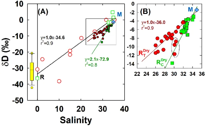
Accordingly, δ18O and δD values in the samples collected in the mangroves of Coco and Temala
269
varied linearly with salinity (Figure 3 and Table 2). In addition, all linear relationships 270
converged to a common signature of the marine endmember (blue diamond in Figure 3). We 271
extrapolated these linear relationships toward salinity of zero to determine the isotope 272
composition of each river water endmember (Table 2). It is important to note that the 273
interpretation of such relationships often requires a spatial and temporal assessment of the two 274
systems (Conroy et al., 2017). As the samples were collected simultaneously in the dry season, 275
the difference in water isotope composition between the freshwater endmembers at Coco and 276
Temala can thus be only attributed to distinct water sources in each river system. 277
In the mangrove stations, the two linear regression lines are significantly distinct between Coco 278
and Temala, except for a few stations at Temala that fall on the regression line of Coco (encircled 279
12 data, Figure 3B). These data represent the last samples collected during the high tide over the 24-280
hour series (3rd discharge event of the Coco River, Figure 2A). All physical-chemical properties
281
and stable water isotopes of the two rivers overlap during this period (grey zone in Figure 2 A, 282
D, G). This probably reflects a common blackish water mass formed during the high tide.
283
Therefore, we excluded these data from Temala’s δD-salinity regression because of the lack of 284
more robust proxies to confirm this phenomenon and assuming that it may be minor. The 285
exclusion of these three data did not affect the fact that the water isotope composition is 286
significantly more depleted in the Coco River than Temala during the dry season. This depletion 287
is more noticeable for δD (-72.9±8.9‰ vs. -36.0±2.8‰, respectively) than δ18O (9.9±1.7‰ vs. -288
8.4±1.2‰, respectively) (Table 2). 289
However, across the estuaries and during the rain season, the δD-S and δ18O-S relationships for
290
both river systems are significantly similar (p<0.05) and align along with consistent equations 291
(δD=1.0×S–33.7 and δ18O =0.2×S–5.2, Table 2 and Figure 3A). Both the slopes and intercepts
292
are close to the Temala mangrove during the dry season (δD=1.0×S–36.0 and δ18O =0.2×S–8.4,
293
Table 2). This observation suggests that the hydrologic regime in the Temala River differs only
294
slightly within seasons with relatively constant water isotope compositions of the river 295
endmember (𝛿𝐷𝑅𝑖𝑣𝑒𝑟𝑇𝑒𝑚𝑎𝑙𝑎 ~ -34 to -36‰ and 𝛿18𝑂
𝑅𝑖𝑣𝑒𝑟𝑇𝑒𝑚𝑎𝑙𝑎 ~ -5.2 to -8.4‰). These values are close
296
to the four southeastern rivers over an annual cycle (Figure 3A) (𝛿𝐷𝑅𝑖𝑣𝑒𝑟𝑆𝐸 = -31 ± 6‰ and
297
𝛿18𝑂
𝑅𝑖𝑣𝑒𝑟𝑆𝐸 = -5.8 ± 1.0‰, Table 2), confirming reasonably consistent δD-S and δ18O-S
298
relationships and hydrologic regimes of major river systems along the western coast of New 299
Caledonia. 300
It is important to note that the Coco River is a small tributary with a relatively dry riverbed with 301
significantly decreased flow during the dry season. Consequently, the Coco River's isotopic 302
compositions differ substantially during the dry and rain seasons (Table 2) due to less 303
precipitation and enhanced evapotranspiration during the dry season. 304
In summary, the difference in stable water isotope composition between the Coco and Temala 305
rivers is related to the natural effects of a depleted hydrologic reservoir with enhanced 306
evaporation. This effect is naturally more noticeable in small reservoirs during the dry season, 307
such as the Coco River than the major streams (Temala and the four southeastern rivers). Overall, 308
13 we observed a relatively conservative hydrologic system with the mixing of only two water 309
masses: the river freshwater and the marine endmembers. Water isotopic data allow excluding the 310
contribution of a third water mass (e.g., groundwater discharge) in these mangrove-dominated 311
estuarine systems. 312
Rare earth element cycling in the mangrove system.
313
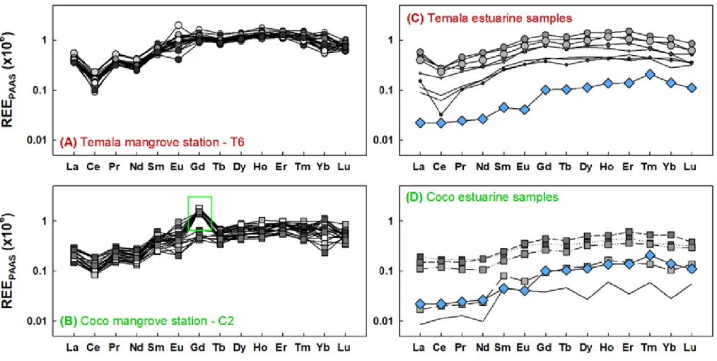
The PAAS-normalized REE patterns are typical of coastal seawater with a gradual enrichment of 314
heavy REEs relative to light REEs (Hoyle et al., 1983; Nozaki et al., 2000; Piper and Bau, 2013) 315
(Figure 4). Moreover, we observed a depletion of Ce but an enrichment of Eu and Gd relative to 316
their neighbouring REEs that are commonly referred to as anomalies. The anomalies of Ce and 317
Eu were already extensively discussed in the literature. The negative Ce anomaly was shown to 318
develop progressively with increasing salinity as dissolved Ce(III) undergoes continued oxidation 319
to insoluble Ce(IV) across the estuarine zone (Nozaki et al., 2000). The positive Eu anomaly was 320
also reported in the dissolved fractions of various major rivers (Amazon, St Lawrence, Piper and 321
Bau, (2013)) and the clay fractions of river sediments worldwide (Bayon et al., 2015). Several 322
previous studies have recorded positive Eu anomaly in continental materials (e.g., suspended 323
load, atmospheric aerosol and dust, Censi et al., 2004; Goldstein and Jacobsen, 1988). Therefore, 324
the positive Eu anomaly observed in the dissolved loads was interpreted as the result of 325
dissolution from suspended particles and formation of stable dissolved complexes during 326
transport (Nozaki et al., 2000). 327
On the other hand, the Gd anomaly is commonly associated with anthropogenic emissions, such 328
as medical sources (medical resonance imagery) or wastewater (Hatje et al., 2016; Tepe et al., 329
2014). We observed Gd anomaly (Gd/Gd* up to 3.5) only during the dry season in the Coco 330
river, in the first and second freshwater discharge events (Figure S3 and Figure 2A). We have 331
previously suggested that the 3rd event may be associated with a common brackish water at both
332
Coco and Temala rivers formed during the high tide from 4h to 9h AM (Figure 2A), which is 333
Gd-anomaly-free (Figure S3D). No Gd anomaly (Gd/Gd* = 1) was indeed observed in the 334
marine endmember (blue diamonds, Figure 4 C,D). Given the absence of major medical facilities 335
and considering the low population along the Coco river, a possible medical or wastewater origin 336
for this Gd anomaly can be ruled out. However, the Coco River is associated with the nickel 337
mined lateritic Koniambo regolith where a 13km long ore conveyor was built parallel to the river 338
14 and the Koniambo Nickel SAS smelting plant is adjacent to the Coco mangrove (Figure 1C). 339
While there is no precedent study reporting Gd anomaly associated with lateritic ores extraction 340
and processing, the Gd anomaly observed in the Coco river might be associated with those 341
activities. 342
Estuarine mixing behaviors of REEs and Y. The REE concentrations in the marine endmembers
343
are typically low; the sum of all REE concentrations (ΣREEs) approximates 6 ng/L. However, 344
there was a significant difference in REE total concentrations between the two river endmembers, 345
with Temala containing more REEs than Coco (ΣREEs of 24 and 2.6 ng/L, respectively). This 346
trend was also observed at the mangrove stations (Figure S3A). The higher REE concentrations 347
measured in the Temala River waters compared to the Coco River are directly associated with the 348
geology of their watersheds. The Temala watershed is indeed made of soils developed on 349
volcano-sedimentary rocks, whereas the Coco river meanders on lateritic soils developed on 350
ultramafic rocks (Figure 1C) (Merrot et al., 2019). As volcaniclastic bedrock tend to contain 351
higher REE and Y concentrations than the granitic regolith (Chapela Lara et al., 2018), the 352
difference in the watershed’s geology could be directly associated with higher REE 353
concentrations in Temala river waters than Coco. 354
Moreover, we did not observe any REEs and Y removal during estuarine mixing between the 355
rivers and the marine endmember, as commonly assumed for REE estuarine geochemistry (see 356
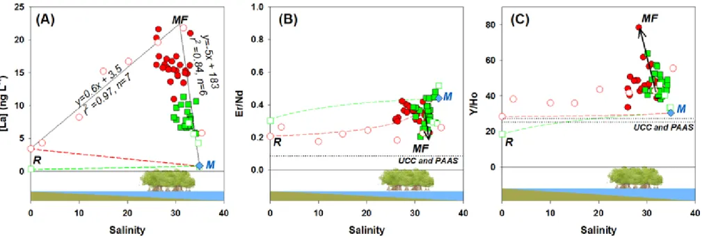
section 1). In fact, we measured very high REE concentrations in the mangrove forest (salinity 357
range of 25-33, see La concentrations in Figure 5A). The high REE (La) concentrations in the 358
mangrove area seem to be conservatively mixed with the freshwater mass (y=0.6x+3.5, r2 = 0.97) 359
and the marine endmember (y=-5.2x+183, r2 = 0.84). This situation was not reported previously.
360
It is commonly assumed that approximately 60-90% of REEs are removed from the low salinity 361
region of an estuary by flocculation/coagulation of dissolved organic-bound Fe and colloidal 362
materials depleting REEs from the dissolved pool (Lawrence and Kamber, 2006; Pourret and 363
Tuduri, 2017; Sholkovitz and Szymczak, 2000; Sholkovitz, 1995). Minor releases of REEs 364
during an estuary mixing were only reported in the turbid-clear water transition zone (S=12-15) 365
in the Chao Phraya estuary (Thailand) (Nozaki et al., 2000) and the mid-salinity zone of the 366
Elimbah Creek (Australia) (Lawrence and Kamber, 2006). Such REE release was attributed to 367
several mechanisms, including desorption from suspended particles, coastal erosion, and 368
15 mineralization during early diagenesis. In addition, the reductive dissolution of ferromanganese 369
oxides has been shown to significantly release REEs into the porewater, although LREEs tend to 370
sorb back onto the newly formed ferromanganese oxides at the sediment-water interface (Och et 371
al., 2014). 372
Although the La-salinity biplots (Figure 5A) could be interpreted as mixing of three water 373
masses (river, mangrove forest, and marine), stable water isotopes (Figure 3) allow to rule out 374
the possibility of a third water mass in the estuaries of Coco and Temala. Thus, the high La 375
concentrations in the mangrove are instead explained by specific biogeochemical processes 376
leading to the substantial release of dissolved REEs. Given the subtropical weather condition and 377
the high availability of fresh organic matter in the mangrove forest (Noël et al., 2014), it is highly 378
probable that bacterial activity contributes to this REEs solubilization in the sediments porewater 379
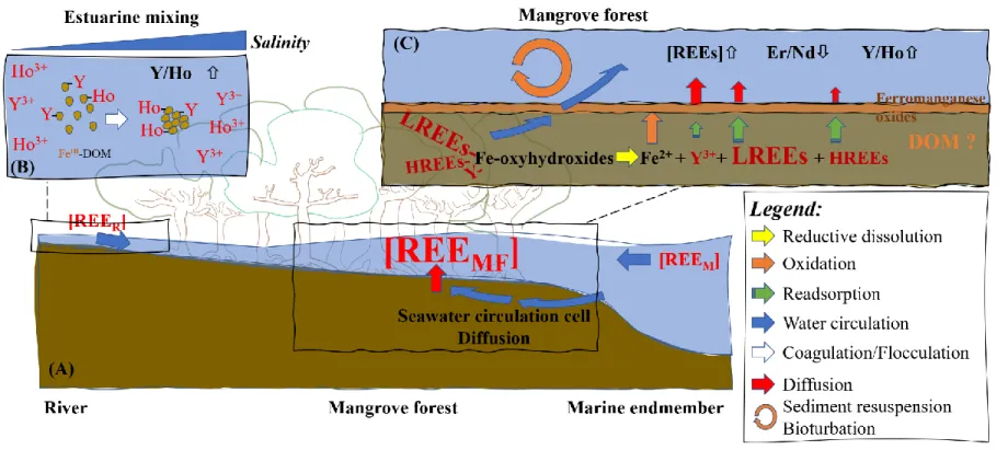
(Och et al., 2014). In the mangrove system, the tidal conditions with water pushing up through 380
the porous sediment (seawater circulation cell, Figure 6A) would then favour REE 381
remobilization to the water column. A previous study has demonstrated significant fluxes of 382
REEs from such a seawater circulation through diagenesis-active sediments (i.e., organic matter 383
degradation and reductive dissolution of ferromanganese oxides (Paffrath et al., 2020), Figure 6). 384
Other processes such as passive diffusion fluxes or sediment resuspension events induced by 385
waves and tides (Dang et al., 2020) or bioturbation could also contribute to the REE release 386
towards the water column (Figure 6 C). At a larger scale of the Northwestern Mediterranean Sea, 387
upward diffusion of REEs (Nd) from sediment porewater counts for 30% of the Nd marine 388
budget (Garcia-Solsona and Jeandel, 2020). Moreover, given the organic mater-rich surface 389
waters in the mangrove system and the high affinity between REEs and dissolved organic carbon 390
(Davranche et al., 2004; Marsac et al., 2010; Pourret and Davranche, 2013), it is also highly 391
possible that the formation of stable organic complexes could contribute to maintaining REEs in 392
solution in this mid-salinity region (25-33). 393
Fractionation of HREEs/LREEs and elemental ratios. All the water samples collected showed
394
a progressive enrichment of HREEs relative to the PAAS shale (Figure 4). This is consistent 395
with the conventional REE behaviours in the aquatic environment where the fractionation 396
between the dissolved and particulate loads of HREEs and LREEs leads to this characteristic 397
REE curve (Piper and Bau, 2013). Therefore, elemental ratios between representative HREEs and 398
16 LREEs (e.g., Er/Nd (Nozaki et al., 2000), Nd/Lu (Sholkovitz, 1995), Ho/Er (Lawrence and
399
Kamber, 2006)) could help determine whether this fractionation occurs in the freshwater 400
endmember or the estuary. As the interpretations using different ratios are very similar, we 401
choose to discuss only the Er/Nd (weight ratios). 402
The Er/Nd ratios in both UCC (Rudnick and Gao, 2003) and PAAS (McLennan, 2001) 403
approximate 0.08, while those in the river endmembers are significantly above this value (0.2 and 404
0.3 at Temala and Coco, respectively, Figure 5B). This indicates that the fractionation between 405
HREEs and LREEs occurred in the freshwater system. It is important to note that such 406
fractionation is pH-dependent. At the pH range observed in Temala and Coco rivers (7.7-7.9, 407
Table 1), REE adsorption on particles is enhanced, leading to significant fractionations by
408
preferential LREE removal (Sholkovitz, 1995). Furthermore, the measured Er/Nd in the estuarine 409
samples varied with salinity along the conservative mixing line of Temala (Figure 5B), 410
suggesting no further fractionation (Lawrence and Kamber, 2006). This is consistent with the 411
occurrence of dissolved organic-REE complexes in the mangrove waters, as previously 412
suggested. Previous studies have demonstrated that the presence of dissolved organic matter 413
significantly reduced REE sorption on ferromanganese oxides and the subsequent fractionation 414
between LREEs and HREEs (Davranche et al., 2005, 2004). 415
On the other hand, a negative departure from the conservative mixing line (i.e., Er/Nd ratios 416
decreased) was noticed at the mangrove stations (black arrow in Figure 5B). This indicates a 417
preferential release of LREEs (Nd) relative to the HREEs (Er). This observation is in agreement 418
with the hypothesis that LREEs previously bound to the solid fraction are released toward 419
solution when the oxide phases undergo reductive dissolution (Bau et al., 1997). High REEs 420
concentrations in porewater promote upward diffusion from the sediments by the seawater 421
circulation cell or diffusive flux (Figure 6). 422
Furthermore, variations in the Y/Ho ratios are also of great interest. Although these two elements 423
have similar ionic radii, their electronic configurations differ. Yttrium has no f-electron while Ho 424
has 10 electrons filling up the f orbitals (Lawrence and Kamber, 2006). Therefore, the ability to 425
form strong surface and solution complexes using the f orbitals (Byrne and Lee, 1993) drives the 426
fractionation of this pair during weathering, riverine transport or in the marine environment 427
17 (Lawrence and Kamber, 2006; Nozaki et al., 2000). As a result, Ho tends to form more stable 428
surface complexes than Y (Bau et al., 1997; Byrne and Lee, 1993; Lawrence and Kamber, 2006). 429
Therefore, two conditions could lead to Y/Ho fractionation during estuarine mixing. First, 430
coagulation, flocculation and sedimentation of Ho-bearing colloidal particles preferentially 431
remove Ho from solution. Second, as Y tends to form weaker surface complexes than Ho, this 432
fractionation is enhanced by the salt effect (competition for surface sorption sites), which favors 433
Y release from colloidal particles toward solution. Both processes were well documented in the 434
literature to support the increase in the Y/Ho ratio during the estuarine mixing (Figure 6B) 435
(Lawrence and Kamber, 2006). 436
The Y/Ho ratio in the Temala river endmember (28.4) approximates UCC and PAAS (25.3 437
(Rudnick and Gao, 2003) and 27.2 (McLennan, 2001), respectively), indicating that there was no 438
significant fractionation between Y and the REEs in the Temala river (Figure 5C) (Lawrence and 439
Kamber, 2006). However, in the Coco river endmember, the Y/Ho ratio is significantly lower 440
(18.6). A situation where Y-Ho fractionation leads to lower Y/Ho ratios relative to the UCC is 441
scarcely reported in the literature. While considered a minor process in natural water systems, it 442
was previously reported by Bau et al. in the slightly acidic solutions of low complex-forming 443
capacity of a stream from an abandoned mine (Bau et al., 1995). Interestingly, the Coco River, 444
where this phenomenon is suspected to occur, is connected to the Koniambo mine. 445
In the estuary, we also observed the conventional Y/Ho fractionation (Figure 6B) as the Y/Ho 446
ratios were beyond the conservative mixing lines (Figure 5C). However, the positive departure is 447
even more noticeable in the mangrove forest, with Y/Ho reaching up to 80 (black arrow in 448
Figure 5C). This suggests that additional processes took place in the mangrove forest area,
449
further fractionating this pair. A previous study has suggested that the fractionation between Y 450
and Ho could be redox driven (Bau et al., 1997). Accordingly, a redox change is expected to 451
occur at the sediment-water interface (Figure 6C) where the upward diffusive flux from 452
mangrove sediments confronts the freshly formed ferromanganese oxyhydroxides. As discussed 453
previously, these reactive surfaces tend to further remove Ho relative to Y. Such preferential 454
removal of Ho increases the Y/Ho ratios as observed in Figure 5C. 455
Calculations of REE flux from the mangrove systems
18 Fluvial fluxes of dissolved constituents in the oceans are essential to balance their marine budget. 457
The current ocean box models for REEs consider major inputs as river-borne dissolved and 458
particulate load, atmospheric dust, groundwater discharge, porewater diffusion and dissolution of 459
reworked sediments (Arsouze et al., 2009; Garcia-Solsona and Jeandel, 2020; Tachikawa et al., 460
2003). 461
Goldstein and Jacobsen have suggested a simple empirical approach to calculate the dissolved 462
REEs flux (𝑅𝑖𝑒𝑓𝑓.) from the continent (Goldstein and Jacobsen, 1988) as detailed in the following 463 equation. 464 𝑅𝑖𝑒𝑓𝑓.= 𝐶𝑖𝑅× 𝐹 𝑅 × 𝜙𝑖 × 𝐶𝐹 (𝐸𝑞. 6) 465
where 𝐶𝑖𝑅 is the dissolved concentration of an element in the continental endmember (ng/L), FR is
466
the annual river discharge, Φi is the effective factor, and CF is a correction factor to convert the
467
final units into kg/year. 468
Here, we applied this calculation to our preliminary dataset to determine whether the fluxes of 469
REEs and Y from the tropical mangrove system could be of interest in the global oceanic budget. 470
Therefore, it is important to note a few assumptions in this simple calculation. First, because of 471
the conservative mixing of REEs and Y between the mangrove system and the seawater (Figure 472
5A), we can assume a full effective factor (i.e., absence of estuarine removal or Φi =1). Second,
473
the local Water Agency (DAVAR, Service de l’eau) monitored the hydrologic regime of the local 474
river systems. According to the most recent report, the monthly discharges of the rivers in the 475
leeward side (southwestern, e.g., Boghen, Poya, Pouembout-Boutana Rivers) of Grand Terre in 476
2019 and 2020 average 18.6 m3/s in February and 0.6 m3/s in May (the month preceding the two 477
sampling campaigns) (DAVAR Service de l’eau, 2020). The variability of the river discharge that 478
could differ Coco and Temala, although not individually determined, could be consisted within 479
the variability of major river systems of the leeward sides. Third, the concentrations of REEs and 480
Y of the mangrove endmember (𝐶𝑖𝑅) are those of the samples with salinity in the range of 25-34
481
(the mangrove forest, Figure 5A). Finally, the calculated fluxes (𝑅𝑖𝑒𝑓𝑓.) of dissolved REEs and Y 482
from the mangrove system are reported with standard deviations reflecting the errors propagating 483
through the calculations and variability of all variables. 484
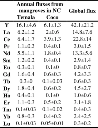
19 Accordingly, 𝑅𝑖𝑒𝑓𝑓. values of Temala and Coco in the dry and rain seasons are reported in Table 485
S3 while the annual average fluxes are showed in Table 3. The fluxes of REEs and Y are
486
significantly higher in the rain season and dry season (Table S3), as reported in other major 487
estuarine systems (Pourret and Tuduri, 2017). Overall, the annual averages of REE and Y fluxes 488
from the Coco and Temala range from 0.05 (Lu) to 16.1 (Y) kg per year (Table 3). 489
To extrapolate our data toward a general perspective of the global mangrove system, we first 490
normalized the calculated fluxes to mangrove watershed surface areas (SW, km2) and the fraction
491
of vegetation coverage (fV). Equation 7 allows the calculation of area-normalized fluxes of REEs
492
and Y from the two mangrove forests (𝑅𝑖𝑆−𝑀𝐹, kg/yr/km2).
493
𝑅𝑖𝑆−𝑀𝐹 = 𝑅𝑖𝑒𝑓𝑓.
𝑆𝑊× 𝑓𝑉(𝐸𝑞. 7) 494
The watershed of the Voh region has a vegetation coverage of approximately 43±16% (Taureau 495
et al., 2019), thus fV =0.43. The surfaces of the Temala and Coco watersheds (SW) approximates
496
163 km2 and 42 km2, respectively (FalconBridge NC, 2001). The calculated area-normalized
497
fluxes of REEs and Y range from 1.6×10⁻³ (Lu) to 0.4 (Y) kg/yr/km2.
498
From the 𝑅𝑖𝑆−𝑀𝐹 values, we attempted an extrapolation to the global surface of mangroves
499
(150,000 km2) (Spalding, 2010) and thus calculated the global fluxes of dissolved REEs and Y 500
from this unique ecosystem (Table 3). These global fluxes calculated for the mangrove systems 501
could then be compared to the published global river-borne dissolved Nd loads (Arsouze et al., 502
2009; Garcia-Solsona and Jeandel, 2020; Tachikawa et al., 2003). Currently, the Nd oceanic 503
budget is the most comprehensive as extensive studies reported both Nd concentrations and 504
isotope composition to calibrate its ocean box models. In these models, the river inputs of 505
dissolved Nd range from 260 to 500 tons per year (or Mg per year) (Rousseau et al., 2015; 506
Tachikawa et al., 2003). Relative to these values, we estimate that the mangrove systems supply 507
13.3±5.6 tons per year of dissolved Nd, representing 2.6-5 % of the total river input of dissolved 508
Nd. Compared to other sources (e.g., dust dissolution of 400 tons of Nd per year, Nd release from 509
suspended particles of 5,700±2,600 ton per year) (Arsouze et al., 2009; Rousseau et al., 2015; 510
Tachikawa et al., 2003), the mangrove systems appear to be a minor source. However, it is 511
important to note that even though this study documents a significant release of REEs and Y 512
20 within the mangrove system for the first time, we assess only two small mangrove systems
513
representing <1% of the global mangrove surface. Further studies are therefore required to better 514
characterize the contribution of the mangrove system to the global marine budget. 515
4. Implications for the role of mangrove on REE cyling and oceanic budgets.
516
The conventional estuarine REE behaviour often implies a sharp removal of REEs when a 517
riverine water mass enters an estuary. However, our data revealed a significantly release of 518
dissolved REEs and Y (7.3 times for Y, 6.4 times for La and 3.3 times for Lu) in the mangrove 519
system. Although other water masses could supply REEs to the water column (e.g., groundwater 520
discharge (Kim and Kim, 2011)), our stable water isotopes data confirm a sole binary mixing 521
between the fresh and seawater endmembers in the mangrove estuaries of New Caledonia. This 522
release of REEs and Y has thus to be associated only with internal recycling or biogeochemical 523
processes within the mangrove forests. This dataset thus strengthens the hypothesis that tropical 524
mangroves act as a source of dissolved REEs and Y to the marine system. 525
This finding first redefines the role of tropical mangroves in the cycling of trace elements at the 526
continent-ocean interface. While mangrove forests are often referred to as a buffer zone to filter 527
trace metals from reaching the open sea (Marchand et al., 2012), this assumption might be valid 528
only for the particulate loading. This specific ecosystem produces large amounts of organic 529
matter that is bioavailable for bacterial degradation (Marchand et al., 2012) and thus boosts early 530
diagenesis. These biogeochemical processes lead to the complex recycling of REE-bearing 531
phases. The reductive dissolution of ferromanganese oxides occurs within the subsurface layers 532
of the sediments and is thus responsible for releasing trace elements (Dang et al., 2015, 2014). 533
However, the redox boundary at the seawater-sediment interface leads to forming a thin layer of 534
newly formed Fe- and Mn-oxyhydroxides with large reactive surface areas that efficiently sorb 535
trace elements and thus minimize their upward diffusive flux (Dang et al., 2015; Rigaud et al., 536
2013). Although we could not evaluate the relative amounts of REEs being diffused upward from 537
the sediment porewaters relative to REEs retained at the interface, the diel variation in oxygen 538
concentrations associated with hypoxia events in the mangrove (Dubuc et al., 2019) strongly 539
suggests that the fraction of REEs being retained would be minor regarding the low stability of 540
Fe- and Mn-oxyhydroxides in such redox-dynamic conditions (Bau et al., 1995). 541
21 Over the past 30 years, several works aimed to understand and revisit REE behaviour during 542
estuarine mixing and accumulation in sediments (Bayon et al., 2015; Lawrence and Kamber, 543
2006; Sholkovitz and Szymczak, 2000; Sholkovitz, 1995). This first dataset reporting REEs 544
release in a tropical mangrove may provide an important insight into the contribution of 545
mangrove forests to the oceanic budgets and mass balance of REEs and Y. However, these box 546
models remain unbalanced with a significant missing flux (e.g., 800 Mg per year) (Tachikawa et 547
al., 2003). Pourret and Tuduri (2017) recently suggested the continental shelves as a potential 548
resource of REEs to be included in the oceanic mass balance of REEs. Moreover, mangrove is 549
growing in 123 tropical and subtropical countries and covers a total surface of 150,000 km2 550
(Spalding, 2010). Our simple flux calculation suggests that this atypical system supplies a 551
significant proportion of REEs toward the oceans (2.6-5% of the global dissolved loading). 552
However, it remains uncertain about the representativity of the Coco and Temala systems of the 553
global mangroves. Therefore, further research on the REE cycling within mangrove systems is 554
needed to determine whether the mangrove estuaries should be considered a significant input in 555
ocean mass budget to balance the global REE distribution. 556
Aknowledgements: The authors thank the Trent University’s Internal Operating Grant (#26090)
557
for financial support to D.D.H. Besides, C.D., F.J., H.L., S.M. and B.O. also acknowledge 558
funding from CRESICA (grant CDEI 2017-2021 - VI-3), CDEI 2017-2021 - VI-3 (grant EC2CO- 559
Bioeffect/Ecodyn/Dril/MicrobiEn ‘’TREMOR’’) and CNRT (grant CSF 9PS2013 560
‘’DYNAMINE’’). We also wish to thank Florence Royer (Ifremer) and Etienne Lopez (Ifremer) 561
for their technical assistance during freshwater sampling in the south, as well as the technical 562
(LAMA, US IMAGO) and administrative staff at IRD Noumea for their help and support relative 563 to field campaigns. 564 565 References 566
Arsouze, T., Dutay, J.-C., Lacan, F., Jeandel, C., 2009. Reconstructing the Nd oceanic cycle 567
using a coupled dynamical – biogeochemical model. Biogeosciences Discuss. 6, 5549–5588. 568
doi:10.5194/bgd-6-5549-2009 569
Auer, G., Reuter, M., Hauzenberger, C.A., Piller, W.E., 2017. The impact of transport processes 570
22 on rare earth element patterns in marine authigenic and biogenic phosphates. Geochim. 571
Cosmochim. Acta 203, 140–156. doi:10.1016/j.gca.2017.01.001 572
Bau, M., Dulski, P., Moller, P., 1995. Yttrium and holmium in South Pacific seawater : vertical 573
distribution and possible fractionation mechanisms. Chemie der Erde - Geochemistrymie der 574
Erde 55, 1–15. 575
Bau, M., Moller, P., Dulski, P., 1997. Yttrium and lanthanides in eastern Mediterranean seawater 576
and their fractionation during redox-cycling. Mar. Chem. 56, 123–131. 577
Bayon, G., Toucanne, S., Skonieczny, C., André, L., Bermell, S., Cheron, S., Dennielou, B., 578
Etoubleau, J., Freslon, N., Gauchery, T., Germain, Y., Jorry, S.J., Ménot, G., Monin, L., 579
Ponzevera, E., Rouget, M.L., Tachikawa, K., Barrat, J.A., 2015. Rare earth elements and 580
neodymium isotopes in world river sediments revisited. Geochim. Cosmochim. Acta 170, 581
17–38. doi:10.1016/j.gca.2015.08.001 582
Byrne, R.H., Lee, J.H., 1993. Comparative yttrium and rare earth element chemistries in 583
seawater. Mar. Chem. doi:10.1016/0304-4203(93)90197-V 584
Censi, P., Mazzola, S., Sprovieri, M., Bonanno, A., Patti, B., Punturo, R., Spoto, S.E., Saiano, F., 585
Alonzo, G., 2004. Rare earth elements distribution in seawater and suspended particulate of 586
the Central Mediterranean Sea. Chem. Ecol. 20, 323–343. 587
doi:10.1080/02757540410001727954 588
Chapela Lara, M., Buss, H.L., Pett-Ridge, J.C., 2018. The effects of lithology on trace element 589
and REE behavior during tropical weathering. Chem. Geol. 500, 88–102. 590
doi:10.1016/j.chemgeo.2018.09.024 591
Conroy, J.L., Cobb, K.M., Lynch-Stieglitz, J., Polissar, P.J., 2014. Constraints on the salinity-592
oxygen isotope relationship in the central tropical Pacific Ocean. Mar. Chem. 161, 26–33. 593
doi:10.1016/j.marchem.2014.02.001 594
Conroy, J.L., Thompson, D.M., Cobb, K.M., Noone, D., Rea, S., Legrande, A.N., 2017. 595
Spatiotemporal variability in the δ18O-salinity relationship of seawater across the tropical 596
Pacific Ocean. Paleoceanography 32, 484–497. doi:10.1002/2016PA003073 597
23 Dang, D.H., Layglon, N., Ferretto, N., Omanović, D., Mullot, J.-U., Lenoble, V., Mounier, S., 598
Garnier, C., 2020. Kinetic processes of copper and lead remobilization during sediment 599
resuspension of marine polluted sediments. Sci. Total Environ. 698, 134120. 600
Dang, D.H., Lenoble, V., Durrieu, G., Mullot, J.-U., Mounier, S., Garnier, C., 2014. Sedimentary 601
dynamics of coastal organic matter: An assessment of the porewater size/reactivity model by 602
spectroscopic techniques. Estuar. Coast. Shelf Sci. 151, 100–111. 603
doi:10.1016/j.ecss.2014.10.002 604
Dang, D.H., Lenoble, V., Durrieu, G., Omanović, D., Mullot, J.-U., Mounier, S., Garnier, C., 605
2015. Seasonal variations of coastal sedimentary trace metals cycling: Insight on the effect 606
of manganese and iron (oxy)hydroxides, sulphide and organic matter. Mar. Pollut. Bull. 92, 607
113–124. doi:10.1016/j.marpolbul.2014.12.048 608
Dang, D.H., Zhang, Z., 2021. Hazardous motherboards: Evolution of electronic technologies and 609
transition in metals contamination. Environ. Pollut. 268, 115731. 610
Dansgaard, W., 1964. Stable isotopes in precipitation. Tellus. doi:10.3402/tellusa.v16i4.8993 611
DAVAR Service de l’eau, 2020. Synthèse Ressource en Eau. 612
Davranche, M., Pourret, O., Gruau, G., Dia, A., 2004. Impact of humate complexation on the 613
adsorption of REE onto Fe oxyhydroxide 277, 271–279. doi:10.1016/j.jcis.2004.04.007 614
Davranche, M., Pourret, O., Gruau, G., Dia, A., Bouhnik-Le Coz, M., 2005. Adsorption of REE 615
(III)-humate complexes onto MnO2: Experimental evidence for cerium anomaly and 616
lanthanide tetrad effect suppression. Geochemistry, Geophys. Geosystems 69, 4825–4835. 617
doi:10.1016/j.gca.2005.06.005 618
Desclaux, T., Lemonnier, H., Genthon, P., Soulard, B., Le Gendre, R., 2018. Suitability of a 619
lumped rainfall–runoff model for flashy tropical watersheds in New Caledonia. Hydrol. Sci. 620
J. 63, 1689–1706. doi:10.1080/02626667.2018.1523613 621
Dublet, G., Juillot, F., Morin, G., Fritsch, E., Noel, V., Brest, J., Brown, G.E., 2014. XAS 622
evidence for Ni sequestration by siderite in a lateritic Ni-deposit from New Caledonia. Am. 623
Mineral. doi:10.2138/am.2014.4625 624
24 Dubuc, A., Baker, R., Marchand, C., Waltham, N.J., Sheaves, M., 2019. Hypoxia in mangroves: 625
Occurrence and impact on valuable tropical fish habitat. Biogeosciences 16, 3959–3976. 626
doi:10.5194/bg-16-3959-2019 627
Elderfield, H., Greaves, M.J., 1982. The rare earth elements in seawater. Nature 296, 214–219. 628
doi:10.1038/296214a0 629
FalconBridge NC, 2001. Projet Koniambo: Carte# 3. Etude environnementale de base. Carte 630
syntese du milieu bio-physique et du milieu marin. 631
Garcia-Solsona, E., Jeandel, C., 2020. Balancing Rare Earth Element distributions in the 632
Northwestern Mediterranean Sea. Chem. Geol. 532, 119372. 633
doi:10.1016/j.chemgeo.2019.119372 634
Goldstein, S.J., Jacobsen, S.B., 1988. Rare earth elements in river waters. Earth Planet. Sci. Lett. 635
89, 35–47. doi:10.1016/0012-821X(88)90031-3 636
Hatje, V., Bruland, K.W., Flegal, A.R., 2016. Increases in Anthropogenic Gadolinium Anomalies 637
and Rare Earth Element Concentrations in San Francisco Bay over a 20 Year Record. 638
Environ. Sci. Technol. 50, 4159–4168. doi:10.1021/acs.est.5b04322 639
Hoyle, J., Elderfield, H., Gledhill, A., Greaves, M., 1983. The behavior of the rare earth elements 640
during mixing of river and sea water. Geochim. Cosmochim. Acta 48, 13–149. 641
Kim, I., Kim, G., 2011. Large fluxes of rare earth elements through submarine groundwater 642
discharge (SGD) from a volcanic island, Jeju, Korea. Mar. Chem. 127, 12–19. 643
doi:10.1016/j.marchem.2011.07.006 644
Lawrence, M.G., Kamber, B.S., 2006. The behaviour of the rare earth elements during estuarine 645
mixing-revisited. Mar. Chem. 100, 147–161. doi:10.1016/j.marchem.2005.11.007 646
Lee, K., Grundstein, A.J., Wenner, D.B., Choi, M., Woo, N., Lee, D., 2003. Climatic controls on 647
the stable isotopic composition of precipitation in Northeast Asia. Clim. Res. 23, 137–148. 648
Lillie, A.R., Brothers, R.N., 1970. The geology of New Caledonia. New Zeal. J. Geol. Geophys. 649
13, 145–183. doi:10.1080/00288306.1970.10428210 650
25 Ma, L., Dang, D.H., Wang, Wei, Evans, R.D., Wang, Wen-xiong, 2019. Rare earth elements in 651
the Pearl River Delta of China: Potential impacts of the REE industry on water, suspended 652
particles and oysters. Environ. Pollut. 244, 190–201. doi:10.1016/j.envpol.2018.10.015 653
Marchand, C., Fernandez, J.M., Moreton, B., Landi, L., Lallier-Vergès, E., Baltzer, F., 2012. The 654
partitioning of transitional metals (Fe, Mn, Ni, Cr) in mangrove sediments downstream of a 655
ferralitized ultramafic watershed (New Caledonia). Chem. Geol. 656
doi:10.1016/j.chemgeo.2012.01.018 657
Marsac, R., Davranche, M., Gruau, G., Dia, A., 2010. Metal loading effect on rare earth element 658
binding to humic acid: Experimental and modelling evidence. Geochim. Cosmochim. Acta 659
74, 1749–1761. doi:10.1016/j.gca.2009.12.006 660
McLennan, S.M., 2001. Relationships between the trace element composition of sedimentary 661
rocks and upper continental crust. Geochemistry, Geophys. Geosystems 2, 2000GC000109. 662
doi:10.1038/scientificamerican0983-130 663
Merrot, P., Juillot, F., Noël, V., Lefebvre, P., Brest, J., Menguy, N., Guigner, J.M., Blondeau, M., 664
Viollier, E., Fernandez, J.M., Moreton, B., Bargar, J.R., Morin, G., 2019. Nickel and iron 665
partitioning between clay minerals, Fe-oxides and Fe-sulfides in lagoon sediments from 666
New Caledonia. Sci. Total Environ. doi:10.1016/j.scitotenv.2019.06.274 667
Munksgaard, N.C., Wurster, C.M., Bass, A., Zagorskis, I., Bird, M.I., 2012. First continuous 668
shipboard δ 18O and δD measurements in sea water by diffusion sampling-cavity ring-down 669
spectrometry. Environ. Chem. Lett. 10, 301–307. doi:10.1007/s10311-012-0371-5 670
Noël, V., Marchand, C., Juillot, F., Ona-Nguema, G., Viollier, E., Marakovic, G., Olivi, L., 671
Delbes, L., Gelebart, F., Morin, G., 2014. EXAFS analysis of iron cycling in mangrove 672
sediments downstream a lateritized ultramafic watershed (Vavouto Bay, New Caledonia). 673
Geochim. Cosmochim. Acta 136, 211–228. doi:10.1016/j.gca.2014.03.019 674
Nozaki, Y., Lerche, D., Alibo, D.S., Snidvongs, A., 2000. The estuarine geochemistry of rare 675
earth elements and indium in the Chao Phraya River, Thailand. Geochim. Cosmochim. Acta 676
64, 3983–3994. doi:10.1016/S0016-7037(00)00473-7 677
26 Och, L.M., Muller, B., Wichser, A., Ulrich, A., Vologina, E.G., Sturm, M., 2014. Rare earth 678
elements in the sediments of Lake Baikal. Chem. Geol. 376, 61–75. 679
doi:10.1016/j.chemgeo.2014.03.018 680
Paffrath, R., Pahnke, K., Behrens, M., Reckhardt, A., Ehlert, C., Schnetger, B., Brumsack, H.-J., 681
2020. Rare Earth Element Behavior in a Sandy Subterranean Estuary of the Southern North 682
Sea. Front. Mar. Sci. 7, 424. doi:10.3389/fmars.2020.00424 683
Piper, D.Z., Bau, M., 2013. Normalized Rare Earth Elements in Water , Sediments , and Wine : 684
Identifying Sources and Environmental Redox Conditions. Am. J. Anal. Chem. 4, 69–83. 685
doi:10.4236/ajac.2013.410A1009 686
Planavsky, N., Bekker, A., Rouxel, O.J., Kamber, B., Hofmann, A., Knudsen, A., Lyons, T.W., 687
2010. Rare Earth Element and yttrium compositions of Archean and Paleoproterozoic Fe 688
formations revisited: New perspectives on the significance and mechanisms of deposition. 689
Geochim. Cosmochim. Acta 74, 6387–6405. doi:10.1016/j.gca.2010.07.021 690
Pourret, O., Davranche, M., 2013. Rare earth element sorption onto hydrous manganese oxide: A 691
modeling study. J. Colloid Interface Sci. 395, 18–23. doi:10.1016/j.jcis.2012.11.054 692
Pourret, O., Tuduri, J., 2017. Continental shelves as potential resource of rare earth elements. Sci. 693
Rep. 7, 1–6. doi:10.1038/s41598-017-06380-z 694
Rigaud, S., Radakovitch, O., Couture, R.-M., Deflandre, B., Cossa, D., Garnier, C., Garnier, J.-695
M., 2013. Mobility and fluxes of trace elements and nutrients at the sediment–water 696
interface of a lagoon under contrasting water column oxygenation conditions. Appl. 697
Geochemistry 31, 35–51. doi:10.1016/j.apgeochem.2012.12.003 698
Rohling, E.J., 2007. Progress in paleosalinity: Overview and presentation of a new approach. 699
Paleoceanography. doi:10.1029/2007PA001437 700
Rousseau, T.C.C., Sonke, J.E., Chmeleff, J., Van Beek, P., Souhaut, M., Boaventura, G., Seyler, 701
P., Jeandel, C., 2015. Rapid neodymium release to marine waters from lithogenic sediments 702
in the Amazon estuary. Nat. Commun. 6. doi:10.1038/ncomms8592 703
Rudnick, R., Gao, S., 2003. Composition of the continental crust, in: Turekian, K.K., Holland, 704
27 H.D. (Eds.), Treatise on Geochemistry. Elsevier Ltd, pp. 1–64.
705
Sholkovitz, E., Szymczak, R., 2000. The estuarine chemistry of rare earth elements: Comparison 706
of the Amazon, Fly, Sepik and the Gulf of Papua systems. Earth Planet. Sci. Lett. 179, 299– 707
309. doi:10.1016/S0012-821X(00)00112-6 708
Sholkovitz, E.R., 1995. The aquatic chemistry of rare earth elements in rivers and estuaries. 709
Aquat. Geochemistry 1, 1–34. doi:10.1007/BF01025229 710
Spalding, M., 2010. World Atlas of Mangroves, World Atlas of Mangroves. 711
doi:10.4324/9781849776608 712
Tachikawa, K., Athias, V., Jeandel, C., 2003. Neodymium budget in the modern ocean and paleo-713
oceanographic implications. J. Geophys. Res. Ocean. 108, 1–13. doi:10.1029/1999jc000285 714
Taureau, F., Robin, M., Proisy, C., Fromard, F., Imbert, D., Debaine, F., 2019. Mapping the 715
mangrove forest canopy using spectral unmixing of very high spatial resolution satellite 716
images. Remote Sens. 11. doi:10.3390/rs11030367 717
Tepe, N., Romero, M., Bau, M., 2014. High-technology metals as emerging contaminants: Strong 718
increase of anthropogenic gadolinium levels in tap water of Berlin, Germany, from 2009 to 719
2012. Appl. Geochemistry 45, 191–197. doi:10.1016/j.apgeochem.2014.04.006 720
Terry, J.P., Wotling, G., 2011. Rain-shadow hydrology: Influences on river flows and flood 721
magnitudes across the central massif divide of La Grande Terre Island, New Caledonia. J. 722
Hydrol. 404, 77–86. doi:10.1016/j.jhydrol.2011.04.022 723
Wallace, M.W., Hood, A., Shuster, A., Greig, A., Planavsky, N.J., Reed, C.P., 2017. 724
Oxygenation history of the Neoproterozoic to early Phanerozoic and the rise of land plants. 725
Earth Planet. Sci. Lett. 466, 12–19. doi:10.1016/j.epsl.2017.02.046 726
Wolfe, B.B., Karst-Riddoch, T.L., Hall, R., Edwards, T., English, M., Palmini, R., Mcgowan, S., 727
Leavitt, P., Vardy, S., 2007. Classification of hydrological regimes of northern floodplain 728
basins (Peace–Athabasca Delta, Canada) from analysis of stable isotopes (d18O, d2H) and 729
water chemistry. Hydrol. Process. 21, 151–168. doi:10.1002/hyp.6229 Classification 730
Yeghicheyan, D., Aubert, D., Bouhnik-Le Coz, M., Chmeleff, J., Delpoux, S., Djouraev, I., 731
28 Granier, G., Lacan, F., Piro, J.L., Rousseau, T., Cloquet, C., Marquet, A., Menniti, C.,
732
Pradoux, C., Freydier, R., Vieira da Silva-Filho, E., Suchorski, K., 2019. A New 733
Interlaboratory Characterisation of Silicon, Rare Earth Elements and Twenty-Two Other 734
Trace Element Concentrations in the Natural River Water Certified Reference Material 735
SLRS-6 (NRC-CNRC). Geostand. Geoanalytical Res. 43, 475–496. doi:10.1111/ggr.12268 736
737
(2) Auer, G.; Reuter, M.; Hauzenberger, C. A.; Piller, W. E. The Impact of Transport 738
Processes on Rare Earth Element Patterns in Marine Authigenic and Biogenic Phosphates. 739
Geochim. Cosmochim. Acta 2017, 203, 140–156.
740
https://doi.org/10.1016/j.gca.2017.01.001. 741
(3) Wallace, M. W.; Hood, A.; Shuster, A.; Greig, A.; Planavsky, N. J.; Reed, C. P. 742
Oxygenation History of the Neoproterozoic to Early Phanerozoic and the Rise of Land 743
Plants. Earth Planet. Sci. Lett. 2017, 466, 12–19. 744
https://doi.org/10.1016/j.epsl.2017.02.046. 745
(4) Planavsky, N.; Bekker, A.; Rouxel, O. J.; Kamber, B.; Hofmann, A.; Knudsen, A.; Lyons, 746
T. W. Rare Earth Element and Yttrium Compositions of Archean and Paleoproterozoic Fe 747
Formations Revisited: New Perspectives on the Significance and Mechanisms of 748
Deposition. Geochim. Cosmochim. Acta 2010, 74 (22), 6387–6405. 749
https://doi.org/10.1016/j.gca.2010.07.021. 750
(5) Tepe, N.; Romero, M.; Bau, M. High-Technology Metals as Emerging Contaminants: 751
Strong Increase of Anthropogenic Gadolinium Levels in Tap Water of Berlin, Germany, 752
from 2009 to 2012. Appl. Geochemistry 2014, 45, 191–197. 753
https://doi.org/10.1016/j.apgeochem.2014.04.006. 754
(6) Dang, D. H.; Zhang, Z. Hazardous Motherboards: Evolution of Electronic Technologies 755
and Transition in Metals Contamination. Environ. Pollut. 2021, 268, 115731. 756
(7) Ma, L.; Dang, D. H.; Wang, W.; Evans, R. D.; Wang, W. Rare Earth Elements in the Pearl 757
River Delta of China: Potential Impacts of the REE Industry on Water, Suspended 758
Particles and Oysters. Environ. Pollut. 2019, 244, 190–201. 759