HAL Id: tel-03144001
https://tel.archives-ouvertes.fr/tel-03144001
Submitted on 17 Feb 2021HAL is a multi-disciplinary open access archive for the deposit and dissemination of sci-entific research documents, whether they are pub-lished or not. The documents may come from teaching and research institutions in France or abroad, or from public or private research centers.
L’archive ouverte pluridisciplinaire HAL, est destinée au dépôt et à la diffusion de documents scientifiques de niveau recherche, publiés ou non, émanant des établissements d’enseignement et de recherche français ou étrangers, des laboratoires publics ou privés.
of scenarios : toward the validation of the autonomous
vehicle
Marc Nabhan
To cite this version:
Marc Nabhan. Models and algorithms for the exploration of the space of scenarios : toward the validation of the autonomous vehicle. Artificial Intelligence [cs.AI]. Université Paris-Saclay, 2020. English. �NNT : 2020UPASG058�. �tel-03144001�
Models and algorithms for the
exploration of the space of
scenarios: toward the validation
of the autonomous vehicle
Thèse de doctorat de l'Université Paris-Saclay
École doctorale n°580, Sciences et Technologies de l'Information et de
la Communication (STIC)
Spécialité de doctorat: Informatique Unité de recherche: Université Paris-Saclay, Inria, Inria Saclay-Île-de-France, 91120, Palaiseau, France Référent: Faculté des sciences d'Orsay
Thèse présentée et soutenue en visioconférence totale,
le 21 décembre 2020, par
Marc NABHAN
Composition du Jury
Sébastien VEREL
Professeur, Université du Littoral Côte d’Opale Président Jin-Kao HAO
Professeur, Université d’Angers Rapporteur & Examinateur Antoine GRALL
Professeur, Université de Technologie de Troyes Rapporteur & Examinateur Dominique QUADRI
Professeure, Université Paris-Saclay Examinatrice
Marc SCHOENAUER
Directeur de recherche, Inria Saclay Directeur de thèse Yves TOURBIER
Ingénieur de recherche, Renault Co-Encadrant & Examinateur Hiba HAGE
Ingénieure de recherche, Renault Co-Encadrante
Thèse de
doctorat
NN
T:
202
0U
PA
SG
05
8
du transport routier. Hypoth´etiquement, ils sont suppos´es augmenter globalement la s´ecurit´e routi`ere. Cependant, ce sont des syst`emes assez complexes, de la coordination de multiples capteurs `a leur fusion, jusqu’`a la loi de commande qui d´ecide des actions que le v´ehicule ex´ecutera. Une d´efaillance peut se produire durant n’importe quel stade de ce processus, ce qui va enclencher une fausse action sur la route. C’est pourquoi chaque composant de ce syst`eme devra ˆetre rigoureusement test´e pour anticiper des d´efaillances potentielles et les ´eliminer.
Les essais de conduite r´eelle sont utilis´es pour tester le v´ehicule sous diverses condi-tions et identifier des d´efaillances sp´ecifiques. Cependant, cette approche ne peut pas ˆetre utilis´ee seule pour compl´eter le processus de validation, en sachant que plusieurs ´etudes ont montr´e qu’il faudrait des si`ecles de conduite continue pour d´emontrer que le taux de d´efaillance du v´ehicule autonome est inf´erieur `a celui du conducteur humain. C’est pourquoi, grˆace `a l’essor des puissances de calcul, des m´ethodes de test par simulation sont utilis´ees pour compl´ementer les essais r´eels, et sont nettement moins ch`eres. Une de ces m´ethodes est la simulation num´erique, qui g´en`ere des donn´ees virtuelles param´etr´ees et recherche de nouvelles situations `a travers un simulateur de conduite.
Le contexte de cette th`ese s’inscrit dans la simulation num´erique. Son objectif est de faciliter la validation de la loi de commande par des tests en MIL (Model-In-the-Loop) o`u l’environnement de la loi de commande est simul´e sans composants physiques. Nous pou-vons donc v´erifier que les actions choisies par le v´ehicule demeurent en s´ecurit´e selon les r`egles de conduite, et valider num´eriquement les exigences de la loi de commande. Pour cela, nous explorons une multitude de sc´enarios, qui sont des combinaisons de param`etres d’entr´ee qui d´efinissent la situation de conduite appel´ee aussi ”use case”, `a travers le simulateur SCANeR Studio.
Cette th`ese CIFRE fait partie d’un projet industriel `a Renault appel´e ADValue. Son objectif est de combiner plusieurs algorithmes mis en comp´etition pour explorer efficace-ment l’espace des param`etres d’entr´ee d’un ”use case” afin d’identifier toutes les zones d´efaillantes. Pour cela, divers mod`eles et algorithmes sont d´evelopp´es pour exploiter les ressources disponibles d’une mani`ere efficace afin d’´eviter de simuler toutes les conditions imaginables pour tous les ”use cases”, ce qui est intraitable en puissances de calcul. Le but de cette th`ese est de contribuer de nouveaux algorithmes et m´ethodes au projet afin d’arriver `a son objectif.
Les principales contributions de cette th`ese sont organis´ees selon trois objectifs:
D´etection de d´efaillance Un algorithme est d´evelopp´e pour identifier un nom-bre maximal de d´efaillances de la loi de commande en explorant l’espace des param`etres d’entr´ee pour un ”use case” donn´e. Pour satisfaire la contrainte industrielle de r´eduire la puissance de calcul globale n´ecessaire, c’est-`a-dire d’utiliser le simulateur le moins possi-ble, un mod`ele de forˆet al´eatoire est utilis´e intensivement en tant que mod`ele ”surrogate”
du simulateur dans une boucle d’optimisation avec l’algorithme d’optimisation CMA-ES. De plus, en raison de manque de flexibilit´e de l’utilisation du simulateur en mode parall`ele au moment de ces travaux, un mod`ele de r´eseau de neurones est utilis´e en tant que mod`ele de substitution du simulateur actuel, sachant que le terme ”simulation” sera n´eanmoins utilis´e.
D´etection de fronti`ere Trois algorithmes sont d´evelopp´es pour identifier des sc´enarios au plus pr`es de la fronti`ere localis´ee entre zones d´efaillantes et non d´efaillantes. En effet, les ”use cases” sont g´en´eralement d´efinis par des entr´ees continues, comme les acc´el´erations et les vitesses des v´ehicules entourant le v´ehicule autonome. L’espace des param`etres d’entr´ee peut donc ˆetre assimil´e `a une partition de zones d´efaillantes et non d´efaillantes s´epar´ees par une fronti`ere `a d´etecter. Chaque algorithme r´epond `a l’objectif d’une mani`ere diff´erente tout en utilisant la mˆeme strat´egie de r´eduction de coˆut de calcul adopt´ee par l’algorithme de d´etection de d´efaillance.
Mod`eles de fronti`ere Trois approches sont consid´er´ees pour identifier analy-tiquement la fronti`ere aussi pr´ecis´ement que possible dans le but de construire des mod`eles `
a la fois performants et explicables par l’interm´ediaire d’´equations et param`etres: r´eseau de neurones, programmation math´ematique lin´eaire avec extensions, et programmation g´en´etique appliqu´ee `a la r´egression symbolique. Ils sont tous construits `a l’aide de sc´enarios d´efaillants et frontaliers tels que ceux identifi´es par les algorithmes pr´ec´edents. Les algorithmes d´evelopp´es pour les deux premiers objectifs sont test´es sur un cas de suivi de v´ehicule, et leurs r´esultats sont compar´es `a la ”v´erit´e terrain” calcul´ee sur une grille compl`ete de l’espace des param`etres d’entr´ee, avec plusieurs m´etriques utilis´ees afin de bien ´evaluer la qualit´e des r´esultats obtenus. Les mod`eles issus du troisi`eme objectif sont test´es sur un cas plus sophistiqu´e avec mise `a jour du simulateur, et sont compar´es en calculant les erreurs de classification totales sur toute la grille. Tous ces algorithmes et mod`eles sont inject´es au projet ADValue pour aider `a la validation du v´ehicule autonome bas´ee sur la simulation de sc´enarios.
Acknowledgements
I would like to begin by expressing my deepest gratitude to all the members of the jury, S´ebastien V´erel, Jin-Kao Hao, Antoine Grall and Dominique Quadri, for taking part in this thesis committee and making themselves available in such short notice. I sincerely thank my reviewers for their professionalism in providing reviews with valuable comments and sugges-tions in a record time.
I am deeply indebted to my PhD advisor Marc Schoenauer for his supervision and guid-ance which greatly helped in the successful completion of this PhD. It was truly an honor to work with you. I am also extremely grateful to my industrial advisors at Renault. Thank you Yves Tourbier for entrusting me with this great opportunity, and Hiba Hage for all the insightful advice during all these years.
I would like to sincerely thank the community of PhD students at Renault, especially Sonia Assou, Matthias Coust´e, Benoˆıt Laussat, Lu Zhao and Clara Gandrez for the good times and atmosphere we had at Renault. Thanks to the whole team at Renault, to Martin Charrier who helped with the successful implementation of my work within the ADValue project, and specifically to Joe Antonios for all the great car rides (and venting out dur-ing hard times) we shared together across the years. Many thanks should also go to Alex Goupilleau, Ricardo Rodriguez and Assad Balima for the great times (and the pints) during all these afterworks, and to Pierre Caillard and Maroun Khoury for always coming up with interesting lunch discussions.
I also extend my sincere thanks to all the TAU team at Inria and the LRI, mainly Mich`ele Sebag, Guillaume Charpiat, Corentin Tallec and Diviyan Kalainathan for all the eye-opening discussions and knowledge shared. Special thanks go to Th´eophile Sanchez who was always a delight to talk to during my time at Inria. Many thanks to Rumana Lakdawala and F´elix Louistisserand for their brief but highly appreciated presence at the start of my PhD.
I gratefully acknowledge the assistance of all my friends during all these years. Particu-larly, I am extremely grateful to Estelle Soueidi for her unparalleled and continuous support that greatly helped me during my PhD journey. I would like to extend my thanks to Cyril Caram for the good times spent during all the meals we shared together. Thanks also go to Maria, Paty, Bahjat, Georges, Yara, Perla, St´ephanie, Hamza, Jo¨elle, Myriam, Nabiha, Nayla, Jad, Ghina, Joey, Ghady, Sandy, (and many others...) for their support.
Finally, and most importantly, I deeply thank my parents and my sisters Linda and Joanna for their unwavering emotional support and unrelenting help during all these years. I dedicate this thesis to you.
1 Introduction 16
1.1 Automation in automotive: a brief history . . . 16
1.2 The benefits of an autonomous vehicle . . . 18
1.3 Levels of autonomous driving . . . 19
1.4 The challenges of an autonomous vehicle . . . 21
1.4.1 Autonomous system description. . . 21
1.4.2 Types of failures . . . 23
1.4.3 Validation techniques . . . 24
1.4.4 V-model and associated validation strategy . . . 27
1.5 Industrial context. . . 29
1.6 Objectives of the thesis . . . 31
2 Scenario-based Validation 33 2.1 Coverage-based methods . . . 34 2.1.1 Parameters ranges . . . 34 2.1.2 Parameters distributions. . . 35 2.2 Falsification-based methods . . . 37 2.2.1 Non-simulation detection . . . 37 2.2.2 Simulation-based detection . . . 39 2.3 Problem setting . . . 40
3 Optimization and Regression 42 3.1 Optimization Algorithms . . . 42
3.1.1 CMA-ES, a Derivative-Free Stochastic Optimization Algorithm . . . . 42
3.1.2 Mixed-Integer Linear Programming. . . 45
3.2 Regression Algorithms . . . 46
3.2.1 Decision Trees and Random Forests . . . 47
3.2.2 Deep Neural Networks . . . 50
4 Methodology and Experimental Conditions 64
4.1 Problem statement . . . 64
4.1.1 Use cases and Scenarios . . . 64
4.1.2 The optimization algorithms . . . 65
4.2 Simulator and Surrogate Models . . . 65
4.3 The Substitution Models . . . 66
4.3.1 Deep Neural Networks as Substitution Models . . . 67
4.3.2 Building the Substitution Models . . . 67
4.4 The Reduced Models . . . 68
4.4.1 Random Forests as Reduced Models . . . 68
4.4.2 Initialization of the Reduced Models . . . 69
4.5 Simulation-based Failure Detection . . . 69
4.5.1 The Tracking Vehicle Use Case . . . 69
4.5.2 Building the Substitution Model . . . 71
4.5.3 The Find All Failures Algorithm . . . 73
4.5.4 The Find One Failure Algorithm. . . 75
4.5.5 Results . . . 76
5 Border Detection 82 5.1 Find Border Pairs . . . 83
5.1.1 Methodology . . . 84
5.1.2 The Find Border Max Algorithm . . . 84
5.1.3 The Find Border Min Algorithm. . . 86
5.2 Find Border Scenarios . . . 86
5.2.1 The Find Border Points Algorithm . . . 86
5.3 Experimental Results. . . 89
5.3.1 Experimental Conditions . . . 90
5.3.2 Quantitative Results – 1 000 simulations. . . 92
5.3.3 Qualitative Results – 1 000 simulations . . . 101
5.3.4 Quantitative Results – 3 000 simulations. . . 116
5.3.5 Qualitative Results – 3 000 simulations . . . 117
5.3.6 Partial conclusion . . . 120
6 Border Models 122 6.1 The NHTSA 13 Use Case . . . 123
6.2 Neural Network Border Models . . . 124
6.2.1 Methodology . . . 125
6.2.2 Results . . . 126
6.2.3 Conclusions regarding Neural Network as Border Models. . . 129
6.3 MILP based Border Models . . . 131
6.3.2 Global MILP Model . . . 131
6.3.3 Iterative MILP Approach . . . 140
6.3.4 Greedy MILP Algorithm. . . 153
6.4 Genetic Programming Border Models. . . 159
6.4.1 Methodology . . . 159
6.4.2 First Results using DEAP . . . 160
6.4.3 Results using TADA . . . 160
6.5 Discussion . . . 165
7 Conclusions 166 7.1 Discussions . . . 169
1.1 SAE J3016 ”Levels of driving automation.” . . . 19
1.2 Autonomous driving systems flow description. . . 22
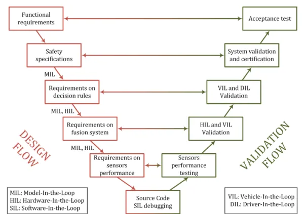
1.3 V-model of the design and validation flows of the ADAS and autonomous driving perception, fusion and decision systems. . . 28
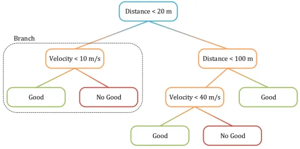
3.1 Visualization of a standard decision tree starting from the root node through the decision nodes leading to the terminal nodes. . . 48
3.2 A multi-layer perceptron. The first layer is the input layer x, whereas the last layer is the output layerby. All the k layers in between are called hidden layers, and each node and edge represent respectively a neuron with its activation function, and a learnable weight. . . 52
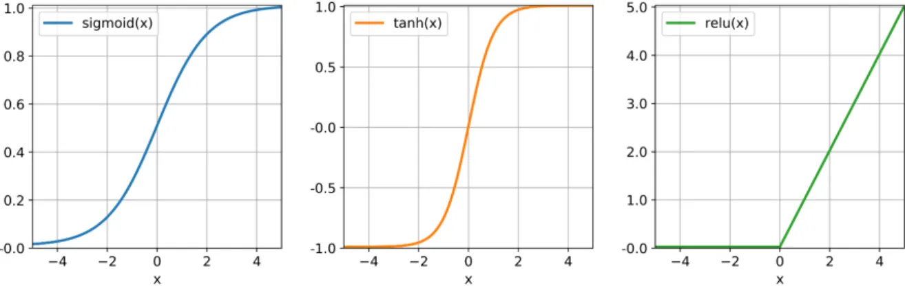
3.3 Illustrations of non-linear activation functions examples used in the implemen-tation of neural networks. . . 53
3.4 Tree representation of the LISP format of Equation 3.10. . . 59
3.5 Basic Evolutionary Algorithm. . . 60
3.6 Example of tree crossover. . . 62
4.1 Tracking vehicle use case where EGO is tracking a preceding vehicle that is performing acceleration and deceleration cycles on the same lane. . . 70
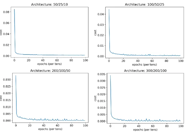
4.2 Evolution of the mean-squared error cost during the epochs for different neural network architectures tested. . . 72
4.3 Flowchart of Find All Failures, which repeatedly detects new faulty scenarios lying as far as possible from the ones from the archive using the embedded Find One Failure optimization algorithm. . . 73
4.4 Evolution of the number of prediction errors related to the Random Forest model during the simulations. The stopping condition is reaching the minimal value of 0.15 a hundred times. . . 74 4.5 Evolution of the distance dobj during the iterations of Find All Failures
algo-rithm that actually resulted in a faulty scenario after evaluation by simulation. The stopping condition is reaching the minimal value of 0.15 a hundred times. 77
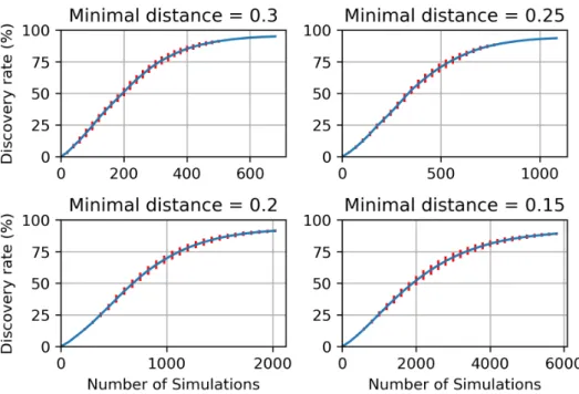
4.6 Mean discovery rates with std. dev. error bars w.r.t. the number of sim-ulations. Each curve is the result of 11 independent runs. Four stopping conditions are represented: 0.3 (top left), 0.25 (top right), 0.2 (bottom left) and 0.15 (bottom right). . . 79 5.1 Flowchart describing the framework of the G/NG pairs detection algorithms
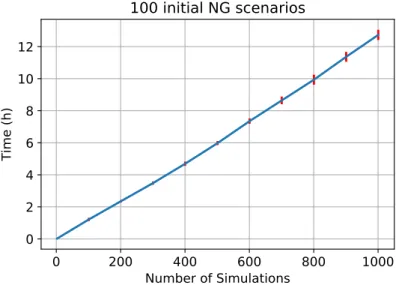
Find Border Max and Find Border Min while using the simulation soft-ware as little as possible. . . 85 5.2 Average time (hours) and standard deviations (vertical bars) spent by Find
Border Max to reach 1,000 simulations. From left to right, initial sets con-taining 50, 100 and 500 NG scenarios. . . 92 5.3 Average time (hours) and standard deviations (vertical bars) spent by Find
Border Max to reach 1,000 simulations for the initial set made of all 32 corners of the scenario space. . . 93 5.4 Average time (hours) and standard deviations (vertical bars) spent by Find
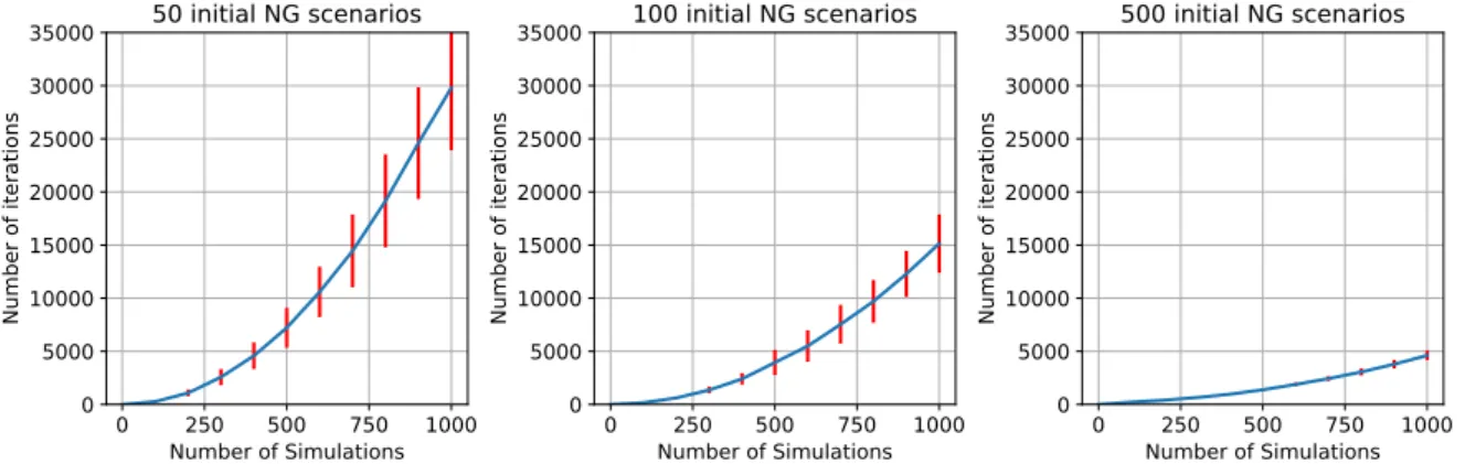
Border Min to reach 1,000 simulations. From left to right, initial sets con-taining 50, 100 and 500 NG scenarios. . . 93 5.5 Average number of iterations (and standard deviations) needed by Find
Bor-der Max to reach 1,000 simulations. From left to right, 50, 100 and 500 NG scenarios. . . 94 5.6 Average number of iterations (and standard deviations) needed by Find
Bor-der Min to reach 1,000 simulations. From left to right, 50, 100 and 500 NG scenarios. . . 94 5.7 Average amount of time in hours (left) and number of iterations (right) spent
by Find Border Min to reach 1,000 simulations with vertical error bars equal to twice the standard deviation values. Each curve is the result of 11 runs with the corners of the use case input space as initial set. . . 95 5.8 Average time (hours) and standard deviations (vertical bars) spent by Find
Border Points to reach 1,000 simulations for the initial set containing 100 NG scenarios. . . 96 5.9 Average number of iterations and standard deviations (vertical bars) spent by
Find Border Points to reach 1,000 simulations for the initial set containing 100 NG scenarios. . . 96 5.10 Evolution of the prediction error rate related to the Random Forest model
based on the initial set containing 100 NG scenarios during 1,000 simulations for the three border detection algorithms. . . 97 5.11 Variation of the number of G/NG scenario couples detected by Find Border
Max for each output criterion throughout the simulations. Each curve is the result of 11 runs with different initial sets containing 50 (top left), 100 (top right) and 500 (bottom left) initial NG scenarios, as well as consisting of the input space corners (bottom right). . . 98
5.12 Variation of the number of G/NG scenario couples detected by Find Border Min for each output criterion throughout the simulations. Each curve is the result of 11 runs with different initial sets containing 50 (top left), 100 (top right) and 500 (bottom left) initial NG scenarios, as well as consisting of the input space corners (bottom right). . . 99 5.13 Number of scenarios (and standard deviations) detected “on” the border by
Find Border Points for each output criterion throughout the simulations, for the initial set containing 100 NG scenarios. . . 100 5.14 Visual explanation of the precision rate: first metric when comparing to the
grid. . . 102 5.15 Variation of the precision rate metric applied on the Find Border Max
algorithm throughout the simulations. Each curve is the result of 11 runs with different initial sets containing 50 (top left), 100 (top right) and 500 (bottom left) initial NG scenarios, as well as consisting of the input space corners (bottom right). . . 103 5.16 Variation of the precision rate metric applied on the Find Border Max
algorithm throughout the simulations by taking into account the 3 and 5 near-est neighbors between the algorithm scenarios. Each curve is the result of 11 runs with different initial sets containing, from left to right, 50, 100, and 500 initial NG scenarios, as well the input space corners. . . 104 5.17 Visual explanation of the border rate: second metric when comparing to the
grid. . . 105 5.18 Variation of the border rate metric applied on the Find Border Points
algorithm throughout the simulations by taking into account the nearest 1, 3 and 5 neighbors between the algorithm scenarios. Each curve is the result of 11 runs with different initial sets containing, from left to right, 1, 50, 100, and 500 initial NG scenarios. . . 106 5.19 Slight offset of the border detected by the algorithm unnoticeable by computing
border rates when comparing to the grid. . . 107 5.20 Visual explanation of the connected components: third and final metric
when comparing to the grid. . . 108 5.21 Variation of the NG classification rate related to the connected components
metric applied on the Find Border Max algorithm throughout the simula-tions by taking into account the nearest 1, 3 and 5 neighbors between the algorithm scenarios. Each curve is the result of 11 runs with different initial sets containing, from left to right, 50, 100, and 500 initial NG scenarios as well as the input space corners. . . 110
5.22 Variation of the NG classification rate related to the connected components metric applied on the Find Border Min algorithm throughout the simula-tions by taking into account the nearest 1, 3 and 5 neighbors between the algorithm scenarios. Each curve is the result of 11 runs with different initial sets containing, from left to right, 50, 100, and 500 initial NG scenarios as well as the input space corners. . . 111 5.23 Variation of the NG classification rate related to the connected components
metric applied on the Find Border Points algorithm throughout the simu-lations by taking into account the nearest 1, 3 and 5 neighbors between the algorithm scenarios. Each curve is the result of 11 runs with different initial sets containing, from left to right, 1, 50, 100, and 500 initial NG scenarios. . 112 5.24 Mean offset distances (and standard deviations) between the original NG
con-nected components and the NG scenarios of the updated concon-nected com-ponents that were incorrectly classified as NG by Find Border Max, Find Border Min and Find Border Points for the different initial sets. . . 114 5.25 Mean coverage distances (and standard deviations) between the undetected
NG scenarios of the original connected components and the NG scenarios of the updated connected components that were correctly classified as NG by Find Border Max, Find Border Min and Find Border Points through-out the simulations. Same initial distribution sets are considered for each algorithm. . . 115 5.26 Average (and standard deviations) of computing times (hours) needed by Find
Border Max, Find Border Min and Find Border Points to perform 3,000 simulations for initial sets containing 500 NG scenarios. . . 117 5.27 Means (and standard deviations) of the NG classification rate related to the
connected components for Find Border Max, Find Border Min and Find Border Points running for 3,000 simulations. . . 118 5.28 Mean coverage distances (and standard deviations) between the undetected
NG scenarios of the original grid connected components and the real NG sce-narios of the updated grid connected components after applying Find Border Max, Find Border Min and Find Border Points within a budget of 3,000 simulations, initial sets containing 500 NG scenarios. . . 118 5.29 Variation of the NG classification rates and mean coverage distances after
combining the scenarios generated by all three algorithms when attempting to reach 3,000 simulations with vertical error bars equal to twice the standard deviation values. Each curve is the result of 11 runs stemming from different initial sets containing 500 NG scenarios. . . 119 6.1 Use case NHTSA 13: Following Vehicle approaching lead vehicle moving at
6.2 Cost function of the Neural Network border model during training phase for an initial set of 10,000 scenarios. . . 126 6.3 Evolution of the cost function of the Neural Network border model during
training phase, while attaining local minima, for an initial set of 10,000 sce-narios: 5,000 border scenarios and 5,000 other scenarios. . . 127 6.4 Variation of the training and test accuracy of the Neural Network throughout
the methodology iterations, trained on an initial set of 10,000 scenarios: 5,000 border scenarios and 5,000 other scenarios. . . 128 6.5 Variation of the error predicted on the border and non-border scenarios of
the 470,587 scenarios of the full grid throughout the methodology iterations, adding up to the total error, using a Neural Network trained on an initial set of 10,000 scenarios: 5,000 border scenarios and 5,000 other scenarios. . . 129 6.6 Training and test accuracy of the Neural Network (left column), and error
predicted on the border and non-border scenarios of the 470,587 scenarios of the full grid (right column) throughout the methodology iterations, trained on initial sets of 5,000, 2,500 and 1,000 containing equally border and other scenarios. . . 130 6.7 2-D representation (left) of the desired MILP model which finds the axes that
separate NG red scenarios from G green scenarios in a tree-like structure (right). . . 132 6.8 Test case #1: The 50 scenarios (left) including G scenarios (green) and a single
NG corner zone (red), and the MILP model (right). . . 134 6.9 Test case #2.1: The 50 scenarios (left) including G scenarios (green) and a
single NG disk zone (red), and the MILP model (right) with δ = 0.01. Notice the third axis at the very bottom right. . . 135 6.10 Test case #2.1: The 50 scenarios (left) including G scenarios (green) and a
single NG disk zone (red), and the MILP model (right) with δ = 0.05. . . . 136 6.11 Test case #2.1: The 50 scenarios (left) including G scenarios (green) and a
single NG disk zone (red), and the MILP model (right) using the quadratic option. . . 136 6.12 Test case #2.2: The 200 scenarios (left) including G scenarios (green) and a
single NG disk zone (red), and the MILP model (right) using the quadratic option. . . 137 6.13 Test case #3: The 200 scenarios (left) including a single NG area (red) located
between two concentric circles separating them from the remaining G (green); the first MILP model (center) with the quadratic option; the second MILP model after introducing 100 new points close to the axes of the first model found (right). . . 138
6.14 One axis edition of MILP realized on test case #2 consisting of 50 scenarios including G scenarios (green) and a single NG disk zone (red). First axis (left) and second axis (right) are found consecutively by the solver with δ = 0.05 and λ = 10. . . 142 6.15 One axis edition of MILP realized on test case #3 consisting of 200 scenarios
including a single NG zone (red) located between two concentric circles sepa-rating them apart from the remaining G (green), while changing the value of the λ hyperparameter (δ = 0.05). . . 143 6.16 One axis edition of MILP realized on test case #3 consisting of 200 scenarios
including a single NG zone (red) located between two concentric circles sepa-rating them apart from the remaining G (green). First axis (left) and second axis (right) are found consecutively by the solver with δ = 0.05 and λ = 1000. 144 6.17 Classes created for the tree representation of the Iterative approach of MILP:
the Node class is parent to the Axis and Cluster classes. . . 145 6.18 Final tree representation of the results of the Iterative MILP approach applied
on test case #4. . . 147 6.19 Step-by-step results of the Iterative MILP approach applied on test case #4
containing two distinct NG areas. . . 148 6.20 Final tree representation of the results of the Iterative MILP approach applied
on test case #5. . . 149 6.21 Step-by-step results of the Iterative MILP approach applied on test case #5
containing three distinct NG areas. . . 150 6.22 Step-by-step results (Part 1) of the Greedy edition of MILP applied on test
case #5 containing three distinct NG areas until reaching its first clustering used. . . 155 6.23 Step-by-step results (Part 2) of the Greedy edition of MILP applied on test
case #5 containing three distinct NG areas after performing its first clustering. 156 6.24 Step-by-step results (Part 3) of the Greedy edition of MILP applied on test
case #5 containing three distinct NG areas until completing the problem. . 157 6.25 Visual representation of the TADA approach on a grid of test case #1 with a
single NG corner area applied to 50, 200 and 500 initial scenarios. . . 161 6.26 Histogram showing the cumulative density probability of the value
“confi-dence” generated by the TADA model on the set of size 10,000 stemming from the use case NHTSA 13. . . 162 6.27 Variation of the accuracy of the TADA model on an initial set of 10,000
sce-narios (5,000 border scesce-narios and 5,000 other scesce-narios) across the iterations of adding lowest confidence scenarios to the initial set. . . 163
6.28 Variation of the total error computed on all 470,587 scenarios of the NHTSA 13 use case after applying the TADA model based an initial set of 10,000 sce-narios (5,000 border scesce-narios and 5,000 other scesce-narios) across the iterations of adding lowest confidence scenarios to the initial set. . . 163
4.1 Description of the input parameters of the tracking vehicle use case. . . 70 4.2 Accuracies of different neural network architectures and hyperparameters (the
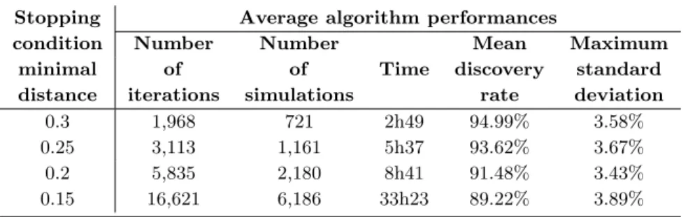
first line being the one chosen for this thesis). . . 72 4.3 Average algorithm performances on 11 runs for each example of stopping
con-dition. . . 80 5.1 Output criteria border boundaries and tolerances for Find Border Points. 89 6.1 Description of the input parameters of the use case NHTSA 13. . . 124 6.2 Global MILP results using Gurobi solver on the NHTSA 13 use case. . . . 139 6.3 Results of the Iterative MILP algorithm on the NHTSA 13 use case. . . 151 6.4 Final prediction of Greedy model using the G and NG trees. . . 158 6.5 Test accuracies (in %) of different models using TADA while changing the
Introduction
1.1
Automation in automotive: a brief history
Before the debut of the electric starter in the 1912 Cadillac Touring Edition, a hand crank and a lot of muscle were needed to start driving a vehicle: Electric starter is considered as one of the most significant innovations in the automobile history. The incorporation of this device into vehicles has set the course for automation in the automotive industry in incremental steps. In 1940, Cadillac and Oldsmobile, both General Motors divisions, followed with the first mass-production of a fully automatic transmission intended for passenger use. They dubbed it the ”Hydra-Matic Drive”, and was considered the greatest advance since the self-starter. Then, in 1958, Chrysler introduced cruise control in motor vehicles. Commonly known as speed control or auto-cruise, it is a system that automatically maintains a selected steady velocity without the use of the accelerator pedal. This system was first available on the Imperial, and was called ”Auto-Pilot”. Another novel system, the Chrysler ”Sure-Brake”, was later unveiled in the Imperial in 1971, and introduced a new dimension to brake engineering. It marked the first production of four-wheel slip control system for passenger cars, after thousands of successful stops were tested on various surfaces at maximum deceleration (Douglas and Schafer,1971).
Nonetheless, the first step toward ”autonomous” driving really took place in the 1990s, when innovation really moved up a gear after some trial and error. First, Mitsubishi released the Debonair in 1991, the first worldwide production car to provide a lidar-based distance warning system. Lidar is a distance measuring method that illuminates its target with laser light and measures the reflected light with a sensor. However, this system only warned the driver about vehicles ahead and did not regulate speed, i.e., no influence over throttle, gear shifting or brakes. Four years later, Mitsubishi unveiled yet another breakthrough after equipping its 1995 Diamante with the first laser ”Preview Distance Control”. This improved system would sense when the closing distance to the vehicle ahead was narrowing, and would automatically regulate speed through throttle control, by easing off the accelerator, and down-shifting to slow down the car. Its key limitation, however, was that it could not operate the
brakes. When the speed difference with the vehicle in front was too great, the only option it had left was to alert the driver with visual and audible warnings. Thus, along with no break-ing intervention, other limitations, e.g., poor performance in the rain, velocity operational limit, propelled Mitsubishi to restrict the system solely for the Japanese market, where the road conditions and generally clement weather were more suitable. European markets had to wait until 1999 for a similar system that befits their roads and weather. That year, the Mercedes-Benz S-Class introduced ”Distronic”, the first radar-assisted Adaptive Cruise Con-trol (ACC). It corrected the biggest limitation of the Japanese system by providing automatic breaking when it detects the car is approaching another vehicle ahead. Its implementation was possible thanks to the development of the computerized Electronic Stability Control (ESC) system by Mercedes that improves vehicle stability by detecting and reducing traction loss. Hence, provisions for automatic braking were already in place. Moreover, Mercedes chose to feature high-quality radar rather than lidar, because it was not affected by rainy, foggy or dusty weather in the way lidar is, and at the same time, was available at a far less expensive cost. Since then, ACC entered multiple iterative improvements to become one of the main foundations of an autonomous vehicle. In the following years, many major automo-tive manufacturers, also known as Original Equipment Manufacturers (OEMs), introduced their own versions of ACC into their cars, including Jaguar, Nissan, Subaru, BMW, Toyota, Renault, Volkswagen, Audi and Cadillac.
After the successful industrialization of the ACC, other features began to be explored and tested. For instance, the Toyota Prius unveiled its Intelligent Parking Assist System option in 2003. This system combined an on-board computer with a rear-mounted camera and power steering in order to automatically accomplish reverse parallel parking with little input from the driver. Another developed feature is the Automatic Emergency Braking (AEB), which is a system that intervenes independently of the driver, and only in critical situations, to avoid or mitigate a potential accident by applying the brakes. These electronic systems, and many others, are called Advanced Driver-Assistance Systems (ADAS), and are designed to aid the vehicle driver while driving or during parking in order to increase car and road safeties. With the successful production of multiple ADAS in just a few short years, the dream of building a fully autonomous vehicle began gradually to materialize. The race toward achieving this dream, and finishing first, had officially begun. Soon enough, many major OEMs started to develop their own autonomous vehicles without revealing their industrial secrets to the pub-lic. Even technology development companies joined the competition later on. For example, Waymo, formerly Google’s Self-Driving Car Project, kicked off the development of their own autonomous driving system in 2009 in secret. They tested their software on Toyota Prius vehicles to try to drive fully and autonomously uninterrupted routes. New electric vehicle companies also decided to participate in the race, notably Tesla with its ”Autopilot” system. Its first version was introduced in 2015 for Model S cars, and it offered multiple ADAS such as lane control with autonomous steering, self-parking and ACC. The system is also able to receive software updates to improve skills over time, until achieving the delivery of full
self-driving at a future time.
In a nutshell, various companies are currently working on their own versions of au-tonomous driving software. The reasons behind this competition are numerous, as various inspiring factors encourage the development of a fully autonomous vehicle.
1.2
The benefits of an autonomous vehicle
First, the main reason for developing a fully autonomous vehicle is to increase road safety. Cars equipped with high levels of autonomy have the potential to mitigate risky human driver behaviors, since they are not subject to distraction, fatigue, excessive speeding or impaired driving. Thus, they can help reduce the number of crashes due to human driver errors, which in turn can save money in the process. Fewer crashes can help avoid their costs, e.g., vehicle repair, medical bills and insurance costs.
Next, full automation can offer greater independence for a lot of people. For instance, highly automated vehicles can help people with disabilities to become self-sufficient in their transportation, and can also enhance independence for seniors. They can increase the pro-ductivity of drivers to recapture time by doing other activities while the car does all the driving. Plus, better transportation services could see the rise in the form of ride-sharing shuttles that provide more affordable mobility by decreasing personal transportation costs. Self-driving car-sharing systems could transform vehicles from personal propriety to a less costly service called on demand.
Moreover, due to the constant population growth and demographic pressure, increasing traffic density is in the foreseeable future. Autonomous vehicles can help in reducing the number of stop-and-go waves that generate road congestion. Because they also mitigate the number of car crashes on the roads, the resulting traffic jams will decrease as well. This could ultimately lead to a better physical and mental health for passengers of self-driving cars. Another factor is the environmental gains that can result from autonomous driving deployment. Besides playing a role in reducing congestion, car-sharing and automation may spur more demand for electrical vehicles. Hence, greenhouse gas emissions can be greatly diluted from needless idling toward a more environmental-friendly future.
Therefore, autonomous vehicles produce many benefits for the safety, independence, pro-ductivity and overall health of passengers on board, as well as the preservation of the envi-ronment. Although they can also have certain negative consequences, like causing job losses on a massive scale, namely taxi drivers and lorry drivers, they could also create new positive outcomes like an increased demand for new jobs, such as software developers and high-tech machine experts. However, all these inspiring factors remain theoretical for the moment. When companies decided to put theory into practice and turn fully autonomous driving into reality, they quickly realized that it was impossible to equip vehicles with highly complex sys-tems all at once unless they address the problem in incremental steps by gradually increasing the autonomy of the car.
1.3
Levels of autonomous driving
For the sake of conceiving fully autonomous vehicles, they have been categorized by the Society of Automotive Engineers (SAE,2018), following levels of driving automation. Each level corresponds to some system complexity that meets the autonomy requirements needed for that level. An Operational Design Domain (ODD) is the set of specific conditions under which a given driving automation system is designed to function, which are different for every level. These conditions include for instance roadway type, traffic conditions and speed range, geographic location, weather and lighting conditions, availability of necessary physical and/or digital supporting infrastructure features, condition of pavement markings and signage...
Six levels of driving automation are defined, from SAE Level 0 (no automation) to SAE Level 5 (full vehicle autonomy) as seen in Figure1.1.
Figure 1.1: SAE J3016 ”Levels of driving automation.”
Levels 0, 1 and 2 are autonomy systems that can be currently found on vehicles on the roads, whereas levels 3, 4 and 5 are still under research with little to no information about their progress due to the great competition between all companies. We will briefly explain
the driver and vehicle roles for each level. • Level 0: No Automation
The driver is in charge of all the driving. The vehicle responds only to inputs from the driver. It can, however, provide warnings about the environment. We find here the well-known systems of past car generations e.g., safety belt, warning lights, ESC, and any other system that leaves us completely in control of our vehicle.
• Level 1: Driver Assistance
The driver must still constantly monitor the drive, but gets basic help in some situa-tions. The system can take over either steering (lane centering feature) or acceleration and deceleration, e.g., ACC and Anti-lock Brake System (ABS). The driver must con-tinuously carry out the other.
• Level 2: Partial Automation
The system can now take over both steering and acceleration and deceleration in some driving situations. The ACC and lane centering features can then be used simultane-ously. The driver must still constantly monitor the drive even when the vehicle assumes these basic driving tasks.
• Level 3: Conditional Automation
The system still takes over both steering, and acceleration and braking in some driving situations. The difference here is that the driver is not needed to constantly monitor the drive anymore. He can partially be distracted from the road like reading a book or texting, but should be ready to resume control of the vehicle within a given time frame if the system so requests. Therefore, the system should be capable of recognizing its limits and notifying the driver appropriately.
• Level 4: High Automation
The driver can hand over the entire driving task to the system. He can take over the system if it is unable to continue, but he is not required to do so, neither for monitoring, nor as backup. The system can assume all driving tasks under nearly all conditions without any driver attention, and will not operate unless the required conditions are met. Although the features can be the same as those found in Level 3, this level gives greater independence for the driver who can freely pursue other activities than concentrating on the road, like sleeping for example.
• Level 5: Full Automation
The system can take over the entire dynamic driving task in all environments under all possible conditions. The features are the same as those found in Level 4. No human driver is required, i.e., the steering wheel is now optional, and everyone can be a passenger in a Level 5 vehicle.
In that way, the problem is divided into incremental steps of driving automation. When a company successfully completes the technical hurdles of a level, it can continue into the next level and update its systems accordingly. The vehicle is equipped with multiple sensors and algorithms that operate coordinately in order to meet the requirements needed for each level. And because the features requested are more and more numerous and challenging, the sensors and algorithms are also more and more numerous and complex. The system must then be robust enough to handle well all situations. Otherwise, system failures could occur, which in turn could lead to car malfunctions that should not be happening. Besides, the trust of future customers is gained once the new system presented is proved to be fully reliable and surely not prone to cause unexpected crashes. Thus, the testing and validation of the autonomous driving systems is mandatory before industrialization. Testing every component should be assessed intensively in order to mitigate potential failures and avoid unwanted problems on the road.
After all, the autonomous vehicle will be one of the first systems to impact user safety without human supervision. Currently, self-piloted systems in aeronautics continue to be constantly supported for any security action. As for the autonomous railway systems, such as the complete automation systems of the metro lines 1 and 14 in Paris, they operate in a closed and well-controlled environment. The level of responsibility can then be shared between the controlled infrastructure and the autonomous systems, unlike for the autonomous vehicle whose environment is open and shared with the rest of the population. Thus, the validation process of the autonomous vehicle is much more complicated than the testing procedures currently found in aeronautics and railway systems.
The next section details how an autonomous vehicle system is designed and how failures could occur during the process, as well as how companies are currently dealing with all the challenges of building a fully autonomous vehicle.
1.4
The challenges of an autonomous vehicle
1.4.1 Autonomous system description
To become autonomous, the vehicle is equipped with a perception system that maps its environment, a fusion system that synchronizes and combines all sensors for a better object detection, and a decision system that controls the actuators following the fusion objects received to indicate the safest trajectory, as illustrated in Figure1.2. All systems are briefly explained next.
1. Perception system
This system consists of a set of sensors from various technologies, e.g., radar, lidar, cam-era, ultrasound, GPS, high definition map or any other existing form of communication technology between vehicles and/or with infrastructure. The sensors are positioned all around the vehicle to give a 360◦ view of its environment. They can be accompanied
Raw data from real environment Sensor 1 Sensor 2 Sensor N Synchroni-zation and Fusion Command law Actuator 1 Actuator 2 Actuator M
Perception Fusion Decision Action
Figure 1.2: Autonomous driving systems flow description.
by an artificial intelligence algorithm which detects elements of infrastructure, side and horizontal road signs, and mobile or motionless road traffic. Each detected object is then tracked, and has a unique identifier per sensor throughout the period during which it is visible to the sensor. If the sensor has seen the object several times, it transmits the information to the fusion system.
However, sensors can give incorrect or imprecise information. They are very sensitive to the real environmental factors, in particular climatic conditions and infrastructure. Therefore, they are usually redundant. The information they transmit is then sup-plemented or repeated by each other, so as to avoid possible objects omission or false objects detection.
2. Fusion system
This system receives the objects detected and transmitted by all sensors. Because of the redundancy of the sensors, the fusion system can reduce the perception errors. First, it synchronizes the data transmitted by the sensors. Then, it merges the redundant information by taking into account the performance of each sensor. Similar to the sensor algorithms, the fusion algorithm also tracks each identified object. The mea-surements performed on this object are then mixed with the predictions from previous measurements. A unique and more precise mapping of the vehicle environment is finally obtained, and is transmitted to the decision system.
3. Decision system
This system takes as inputs all final objects, as identified and transmitted by the fusion system. It takes into account any road sign detected, and predicts the trajectories or the
intentions of other traffic vehicles. It computes what the vehicle should do on the road given all the information provided from the vehicle environment following a predefined command law. Then, it commands the vehicle of the decisions taken and the desired path in the form of instructions transcribed to the vehicle steering wheel, accelerator, and brakes.
4. Actuators
The actuators are the mechanical parts of the vehicle that perform all requested ma-neuvers by the decision system.
The autonomous vehicle represents a highly complex system, from the coordination of its various sensors to their fusion, leading to the decision system which ultimately decides the action to be executed by the vehicle. A failure can occur during any stage of this process, which will result in a wrong behavior on the road.
1.4.2 Types of failures
We list a set of different types of errors that can cause the autonomous vehicle to fail, from all different blocks of the vehicle system anatomy to the requirements needed depending on the levels of autonomy.
• Perception system errors: As previously mentioned, the perception system is greatly impacted or disturbed by environmental factors, which can cause multiple errors: false detections, non-detections or late detections, measurement errors in objects positions and trajectories, sensor loss resulting in a dangerous stop of the autonomous mode... False detections are commonly named false positives, i.e., an object that does not exist is detected, while non-detections are called false negatives, i.e., an object that should be identified is not detected. All of these errors can cause unexpected damages to the vehicle and its passengers.
• Fusion system errors: Since the performances of the sensors vary depending on the environment, a sensor that is generally considered unreliable may be more accurate than others for specific road conditions. The fusion system, whose role is to merge all information transmitted by the perception system to obtain a unique mapping of the vehicle environment, may overlook this sensor and provide an unreliable final mapping to the decision system.
• Misinterpretation of the decision system: Beside the bugs that can be found in the development of the decision algorithm, the decision system may misinterpret the inputs provided by the fusion system, such as the intentions of other traffic vehicles, and transmit erroneous commands to the actuators. This typically happens when the decision system faces a new driving situation with a vehicle environment mapping not
encountered before. Its command law does not cover the exact procedures to transmit to the actuators, despite a perfect functioning of the perception and fusion systems. • Actuator latency: The reaction speed of the actuators fluctuates with its
environ-ment. For example, the ground can be slippery. The braking speed is then impacted, and the decision system may not be able to anticipate the outcome of the present situation.
• Conditional and high automations (Levels 3 and 4) emergency situations: As we have seen in Section 1.3, the system should be capable of recognizing its operating range limits. In the case of level 3 autonomy, the system should notify the driver to take over control of the vehicle, but the driver may not be ready to do so. For level 4 autonomy, the vehicle should handle the situations where the required conditions for its functioning are not met. In both cases, the system must stop the vehicle safely and park it in a safe place. However, this exit may be linked to an end of the authorized use for the autonomous mode, which can result in perturbations in the vehicle behavior. Besides, level 3 is currently described as being the most dangerous autonomy level, because of its conditional status and passing of command between the driver and the vehicle.
These errors are examples that may occur at any time during driving and have then serious consequences on the safety of passengers aboard as well as those involved in road traffic. They are called failures of the autonomous system. It can be impossible to trace which component is responsible for the failure, due to the complexity of the system as a whole. This is why extensive testing and validation are required for each component and at industrialization step.
1.4.3 Validation techniques
As we have noticed so far, the validation of ADAS and autonomous driving systems will occur in highly complex traffic situations. Naturally, software testing is realized on the million lines of codes included in all algorithms of the autonomous driving perception, fusion and decision systems. Possible unwanted software bugs are then eliminated by this source code testing. However, this is not enough to ensure quality testing, as the testing of the autonomous vehicles faces numerous challenges (Koopman and Wagner,2016;Koopman and Wagner, 2017; Koopman and Wagner, 2018). The vehicle should be assessed in real driving situations to know whether or not it is making the right decisions on the road, and what possible failure implications could follow. However, due to the increase in computing power nowadays, numerical models, simulations and virtual simulators can also be used to test autonomous vehicle functions (Belbachir et al., 2012). These are the main categories of validation used nowadays for the validation of the autonomous vehicle, and are more detailed next. Due to the fast evolution of this field, some publications tried to provide a
comprehensive literature review of the different new safety validation methods within these categories (Huang et al.,2016;Junietz et al.,2018;Riedmaier et al.,2020).
1. Real test-driving
The engineering team at Renault, and every other major car company, rely on real test-driving under various conditions in order to validate the autonomous vehicle. Their main objective is to detect specific system failures during these tests. Then, these failures can be eliminated by updating the system accordingly. This complete test database is conducted at different milestones identified in the design process.
Two main sub-categories constitute real test-driving methods.
• Public road testing: Autonomous driving cars can be tested in real open en-vironments. For instance, Google mostly carries out real traffic testing for its self-driving cars. Although it is considered useful in going through realistic and probable driving situations easily, it is also very dangerous in case of a failure resulting in a serious accident. Such was the case for the infamous pedestrian fatality involving an Uber test-vehicle in March 2018. The vehicle was operating in autonomous mode in a neighborhood in Arizona with a human backup sitting in the driver seat. Plus, on-road driving of autonomous vehicles requires new regulations and road traffic rules. Some countries, such as Australia, Germany, France, and the United States, began developing such regulations which can allow on-road testing of autonomous vehicles. Nonetheless, a globally harmonized ap-proach has not yet been developed, as there are differences regarding liability and safety provisions (Lee and Hess,2020).
• Closed course testing: Another way of testing candidate autonomous vehicles in real situations is within closed tracks. There even exists entire testing centers that are dedicated to this method of validation. For example, Mcity is a mock city built for the testing of self-driving cars that is located in the University of Michigan North campus. This technique is safer, obviously, since everything can be controlled on the course. However, it is not scalable, i.e., it can only test driving conditions that humans have thought of and can physically pursue.
Moreover, real test-driving faces a primordial issue for the long run. In fact, the space of possible driving situations is broken down into use cases. Each use case corresponds to a certain driving situation of the autonomous vehicle, such as an insertion of the autonomous vehicle in a lane, or a cut-in of another vehicle in front of the autonomous vehicle. And for every use case, there are multiple possible scenarios that depend on the traffic situation, road description, environment description, vehicle description... Thus, real test-driving is long and expensive, as it is necessary to reproduce accurately all the imaginable conditions, e.g. weather and traffic, that an autonomous vehicle can encounter. Besides, autonomous vehicles should have a lower accident probability than
human drivers for their launch on the market to be socially accepted (Junietz et al.,
2019). Studies have shown that at least 8.8 billion miles (14 billion of kilometers) of test driving are needed to demonstrate with 95% confidence that the autonomous vehicle failure rate is lower than the human driver failure rate (Kalra and Paddock, 2016). Even with a fleet of 100 autonomous vehicles, test-driven 24 hours a day, 365 days a year, this would take about 400 to 500 years.
Hence, it is almost impossible to validate the self-driving cars using real test-driving alone, paving the path for the development of scenario-based validation techniques using models and simulations.
2. Simulation testing
As discussed previously, real test-driving will not be able to cover all imaginable sce-narios for the autonomous vehicle in a reasonable amount of time. Simulation testing methods must hence be used for that goal. They are also way cheaper. We differentiate three main methods of validation techniques by simulation.
• Resimulation: Real test-driving data are injected into a numerical model of the command law to try to replicate them in an open loop. It is mostly useful to carry out non regression tests. This will ensure that the algorithm of the decision system still performs well after some upgrade. Nonetheless, closing this loop remains challenging. For instance, we have in our hands a cut-in scenario of a vehicle in front of the autonomous vehicle driving at constant speed. If a new updated algorithm decides the vehicle should accelerate instead, the vehicle could decide not to realize the cut-in eventually. Thus, it would be useful to change the parameters of the real test-driving data in order to predict more realistic scenarios. Nonetheless, the technical hurdles in modifying raw data visuals or sensors objects and trajectories, while trying to stay realistic, remains quite a challenge nowadays. Therefore, closed-loop resimulation remains a research and development subject. • Numerical simulation: In contrast, this approach is entirely virtual. It
gener-ates virtual parameterized data, so it can create new tests which were unavailable in the original test database. The key advantage of this method is that it is a closed loop. The tests are directly launched into a simulation loop, meaning that certain input parameters can easily be changed in order to cover all possible con-ditions for a certain use case. All past and future events are known at each time step, and can be reproduced and modified. Plus, it is easy to merge multiple simulation models and take advantage of reusing existing results. However, the main drawback of this method is that all results are only valid with respect to the models of the vehicle employed, e.g. all autonomous and dynamic systems, and their degree of realism (Stellet et al., 2015). Further research should determine how to quantify and assess the level of realism of a simulation environment. Until
then, these models are being developed to try to replicate as much as possible the realism of the real systems on the road. Reference by simulation is used, which involves generating synthetically virtual ground truth data that can be compared with real ground truth data to ensure that we have correlation between physical testing and numerical simulation.
• Virtual simulator: A person is driving a real vehicle which is connected to its environment through a simulator software using virtual reality glasses or 180◦ high-resolution screens. This technique is useful in studying the ergonomics and behavior of the driver using autonomous driving mode, while realism of the scenes remains the number one challenge.
Therefore, new and efficient testing methods have been thought through in order to use real test-driving together with simulation to help covering various conditions of the miles needed (Vishnukumar et al.,2017). They are also used to validate each system at a time due to the high complexity of the self-driving vehicle. These available methods are used at each step of the industrial V-model dedicated to the validation of the autonomous driving system (Lakomicki,2018).
1.4.4 V-model and associated validation strategy
Figure 1.3 shows the V-model that can be applied to the validation of the autonomous vehicle and ADAS features. We will detail each step of the diagram next.
1. Requirements on the decision system
All driving rules, which the autonomous vehicle must respect, are elaborated to satisfy high level functional requirements translated into safety specifications. Then, require-ments on decision rules are set, and the behavior of the autonomous vehicle in a given use case is modeled, e.g., its insertion in a lane. This is called Model-In-the-Loop (MIL) testing, which means the model and its environment are simulated with the absence of physical hardware components. The use case is defined by key simulator inputs that characterize the autonomous vehicle environment, and can be modified within a loop to test many possible scenarios generated automatically for a single use case. In that way, we can verify that the actions chosen by the vehicle remain safe according to the driving rules. Hence, these simulations make it possible to test the decision system and numerically validate its requirements while exploring a multitude of scenarios for a defined use case. This is the context of this PhD thesis, and we will get right back to it just after getting through remaining key diagram steps.
2. Requirements on fusion and perception systems
A finer modeling of the data obtained by the fusion system can be added in the MIL to address the requirements on the fusion system. The detection time should be respected,
Figure 1.3: V-model of the design and validation flows of the ADAS and autonomous driving perception, fusion and decision systems.
as well as the obstructions of possible objects that could disturb the sensors. It can even integrate perception errors after fusion. For instance, objects measurements could be noisy, and false positives and false negatives could occur. Thus, failure criteria for the fusion system can be deducted, such as a maximum measurement error, or a maximum detection period, not to be exceeded. In order to include latency or other electronic errors, the real electronic components are integrated. This is called Hardware-In-the-Loop (HIL) simulations.
Then, MIL and HIL simulations are completed with sensors objects data by includ-ing the sensors algorithms. We are now at the perception system output level. The synchronization and fusion stages are thus evaluated. To verify the vehicle robustness, the sensors errors are also modeled like the fusion outputs. A first validation of the fusion system can be realized so that sensors requirements are defined, such as sensors perception reliability.
3. Debugging and validation start
Software-In-the-Loop (SIL) simulations qualify the reliability of the software imple-mented in the embedded system by checking for potential bugs and correcting them. At this stage, the design flow concludes and the validation flow begins where the
sen-sors performance is tested by evaluating their electronic hardware reliability and sensen-sors perception accuracy. Although these can be realized by their respective suppliers, the sensors algorithms performance, e.g., objects detection and classification, rely heavily on their integration in the vehicle and on the environment conditions. Tests should thus be conducted on each sensor already integrated in the vehicle to assess their errors and impacts on the proper functioning of the vehicle. This is important because any error of a sensor can have repercussions on the fusion system too. HIL validation is also conducted to better validate the requirements on fusion system.
4. Decision system validation and final tests
The validation of the decision system is not limited to robustness issues linked to a lack of precision in the perception and fusion outputs, but must also integrate the real actions of the vehicle. It must also be able to emit a clear request to the driver to take control of the driving in the case of Level 3 autonomy for example, and guarantee that this intermediate phase takes place normally and safely. Hence, Vehicle-In-the-Loop (VIL) simulations are used to integrate the real behavior of the vehicle actuators by merging on-road testing and simulated elements. The vehicle is tested on a physical track, but the scenario remains numerical through augmented reality while real tra-jectories are taken into account. Thus, VIL validation is used to further validate the requirements on fusion and decision system simultaneously. Finally, Driver-In-the-Loop (DIL) simulations test the interactions between the driver and the autonomous vehicle. The driver is in a realistic traffic simulator where all his reactions are analyzed during driving, therefore allowing to validate the ergonomics of the human-machine interface while verifying the requirements on decision rules, to verify the security of requests emitted, and to ensure the comfort of the passengers aboard the autonomous vehicle by analyzing their sense of security. Complete system validation and acceptance test are lastly conducted to globally assess the high level safety specifications and functional requirements after completing all past validation steps.
1.5
Industrial context
People at Renault are highly interested in investing in autonomous driving simulation to aid real test-driving in the validation of the autonomous driving mode. A complete validation chain has been defined to address growing technology complexity and use cases diversity. First, use cases are defined through field tests, accident databases, expert knowledge, and global research projects such as Pegasus (P¨utz et al., 2017) to form a use case catalog. This catalog defines each use case, as well as the inputs that characterize the parameters influencing the autonomous vehicle environment. Scenarios can then be generated for a single use case by choosing certain values for all inputs, and can be launched into an in-house simulation software called SCANeR Studio (AVSimulation,2017). It is a software dedicated
to simulation and testing for ADAS and autonomous driving. It provides various tools to run realistic simulations. Numerical vehicle models and sensor models are also built and integrated into the software.
In addition, in order to be able to launch multiple scenarios at the same time, a massive simulation platform is being built. For that aim, thousands of High-Performance Computing (HPC) cores and tens of petabytes of storage capacity will be available by 2025. The SCANeR software as well as all models built are integrated into this platform. We can also integrate the decision system algorithm to the software. Hence, we will have all what it takes to perform a MIL simulation to validate the decision system for a particular use case by 2025 as detailed in previous Section. We set the required software inputs of the use case at the start of the scenario. These inputs are variables that are exterior to the autonomous vehicle, and define its environment. Then, we verify if the autonomous vehicle performs correct and safe actions during the simulation by checking that the output of the simulator satisfies some safety criteria. If not, we have uncovered a failure for this scenario, i.e., this particular combination of inputs for this use case. The decision system should then be corrected in order to take this scenario into account, and avoid obtaining a failure if we run the same simulation of that same scenario with the updated decision system.
Launching a massive simulation plan has become more and more accessible, which is useful to complement real test-driving. As discussed in Section 1.4.3, physical tests can easily validate scenarios that are the most encountered on the road. Simulation should thus be used to cover remaining combinations of input variables that were not tested on the road and detect unlikely edge scenarios, which would otherwise be too costly to validate entirely with real test-driving. However, the dimension of a use case, i.e., the number of input variables that characterize the use case, varies depending on the use case complexity. For some use cases, their dimension can be very high with a wide range of possible values for all inputs. Although possible, simulating all imaginable conditions (up to an acceptable precision for continuous variables) of all use cases can be highly expensive in terms of computing power needed, which is where this thesis comes in.
The goal of this PhD thesis is to facilitate the validation of the decision system by aiding its MIL simulations in exploring the use case input space. In other words, instead of launching a huge number of scenarios and consuming a too large amount of computing power, we want to directly detect combinations of inputs for a particular use case, that will result in a failure of the behavior of the vehicle due to wrong decisions from the decision system during the simulation. These scenarios should include edge cases which represent rare driving circumstances that the actual decision system version has not yet encountered, and can then be eliminated by updating the decision system command law accordingly. Therefore, the complete process of the decision system validation would be to gradually update the command law to decrease the number of failures identified. It is expected that less and less failures would exist as the process goes on – even though the data for only one single step of this overall process (i.e., one single instance of command law) was available at the time of this
work.
This thesis is part of an industrial project at Renault called ADValue (Tourbier, 2017). The project aims at combining multiple algorithms that compete in efficiently exploring the use case input space so as to cover all failure zones in a clever way. In short, our goal is to take a demonstrably smart approach of validating all possible driving conditions while efficiently using time and available resources. In the end, the aim of the thesis is to feed the industrial project with novel algorithms and methods to achieve its objective.
1.6
Objectives of the thesis
All algorithms and models developed during this thesis will be added to the ADValue project in a cooperative way, with the goal of providing a complete tool of numerical validation of the decision system using MIL simulations. They can be divided into three main categories depending on their specific objectives. They will be detailed and addressed in turn in the remaining of this document.
1. Failure detection
This algorithm is developed to explore the input search space for a given use case, and detect as many failures of the autonomous vehicle command law as possible during the simulations. A crucial industrial restriction is added, which is to run as few numer-ical simulations as possible in order to minimize the computational cost. Thus, the final algorithm should be fast and inexpensive, while being efficient in finding a high number of command law failures caused by scattered input conditions. To achieve this objective, an optimization algorithm and a machine learning model are used through an optimization loop (Nabhan et al.,2019).
2. Border detection
Since the inputs that characterize a use case can be of continuous nature, e.g., velocity and acceleration of the traffic vehicles surrounding the autonomous vehicle, the use case input space can then be seen as a partition of the input space into zones where some combinations of inputs ranges lead to a failure, and others where all scenarios are error-free. A more ambitious objective of the domain experts is then to try to detect the border between such faulty and non-faulty areas, i.e., scenarios that are located near such borders. The rationale behind this is to be able to understand the failures of the command law in depth, and correct it once for whole failure areas, rather than making corrections for one failure after another. Three algorithms are developed for that sake. Each of them addresses the objective in a different way. The models and approach used for the failure detection to reduce computing power are also used here. 3. Border models