HAL Id: tel-03153445
https://tel.archives-ouvertes.fr/tel-03153445
Submitted on 26 Feb 2021
HAL is a multi-disciplinary open access archive for the deposit and dissemination of sci-entific research documents, whether they are pub-lished or not. The documents may come from teaching and research institutions in France or abroad, or from public or private research centers.
L’archive ouverte pluridisciplinaire HAL, est destinée au dépôt et à la diffusion de documents scientifiques de niveau recherche, publiés ou non, émanant des établissements d’enseignement et de recherche français ou étrangers, des laboratoires publics ou privés.
To cite this version:
Yannick Le Cacheux. Vers un apprentissage sans exemple plus réaliste. Intelligence artificielle [cs.AI]. Conservatoire national des arts et metiers - CNAM, 2020. Français. �NNT : 2020CNAM1282�. �tel-03153445�
TH`
ESE DE DOCTORAT
pr´esent´ee par :
Yannick LE CACHEUX
soutenue le :10 d´
ecembre 2020
pour obtenir le grade de : Docteur du Conservatoire National des Arts et M´etiers Discipline : Informatique
Sp´ecialit´e : Apprentissage automatique
Toward more practical
zero-shot learning
TH`ESE dirig´ee par
M. Crucianu Michel Professeur des Universit´es, CNAM
et co-encadr´ee par
M. Le Borgne Herv´e Charg´e de recherche, CEA
RAPPORTEURS
M. Jurie Fr´ed´eric Professeur des Universit´es, Universit´e de Caen-Normandie
M. Gravier Guillaume Directeur de recherche, CNRS
PR´ESIDENT DU JURY
Mme Hudelot C´eline Professeur des Universit´es, CentraleSup´elec EXAMINATEURS
Cette th`ese a ´et´e effectu´ee au Laboratoire d’Analyse S´emantique Texte Image (LASTI) du Commis-sariat `a l’ ´Energie Atomique (CEA), membre de l’Universit´e Paris-Saclay, ainsi qu’au Centre d’´Etudes et de Recherche en Informatique et Communications (CEDRIC) du Conservatoire National des Arts et M´etiers (CNAM).
Je tiens tout d’abord `a remercier mes deux encadrants de th`ese, Michel Crucianu et Herv´e Le Borgne, pour leur patience, leur gentillesse et leur disponibilit´e tout au long de la th`ese. Ce fut un plaisir de travailler avec eux.
Je remercie Fr´ed´eric Jurie et Guillaume Gravier pour avoir accept´e de rapporter mon manuscrit. Je remercie ´egalement les autres examinateurs Hichem Sahbi et C´eline Hudelot, qui m’ont fait l’honneur de participer `a mon jury.
Je remercie tous mes coll`egues et amis du laboratoire, pour les ´echanges fructueux et discussions passionnantes que j’ai eu la chance d’avoir avec eux.
Je remercie Coline pour sa pr´esence et son soutien durant toute la dur´ee de ma th`ese.
Je remercie mes colocataires Rapha¨el et Adrien pour les moments de d´etente n´ecessaires pour faire diminuer la pression. Je remercie ´egalement tous les amis sur qui j’ai eu la chance de pouvoir compter pendant cette p´eriode, et dont la liste exhaustive serait bien trop longue.
Enfin, je remercie mes parents, mon fr`ere et ma soeur, ma grand-m`ere et mon grand-p`ere, ainsi que l’ensemble de ma famille pour leur soutien et leur amour durant la th`ese et toutes les ann´ees qui ont pr´ec´ed´ees.
Cette th`ese porte sur la reconnaissance visuelle « zero-shot », qui vise `a classifier des images de cat´egories non rencontr´ees par le mod`ele pendant la phase d’apprentissage. Apr`es avoir class´e les m´ eth-odes existantes en trois grandes cat´egories, nous d´efendons l’id´ee que les m´ethodes dites de classement se basent habituellement sur plusieurs hypoth`eses implicites pr´ejudiciables. Nous proposons d’adapter leur fonction de coˆut pour leur permettre d’int´egrer des relations inter et intra-classe. Nous proposons ´egalement un processus permettant de diminuer l’´ecart entre les performances sur les classes vues et non vues dont souffrent fr´equemment ces m´ethodes. Dans notre ´evaluation exp´erimentale, ces contri-butions permettent `a notre mod`ele d’´egaler ou surpasser les performances des m´ethodes g´en´eratives, tant en ´etant moins restrictif. Dans un second temps, nous nous int´eressons aux repr´esentations s´ e-mantiques utilis´ees dans un contexte d’application `a grande ´echelle. Dans ce contexte, l’information s´emantique provient g´en´eralement de plongements lexicaux des noms de classe. Nous soutenons que les plongements habituels souffrent d’un manque de contenu visuel dans les corpus servant `a leur ap-prentissage. Nous proposons donc de nouveaux corpus de texte davantage connot´es visuellement, ainsi qu’une m´ethode permettant d’adapter les mod`eles de plongement `a ces corpus. Nous proposons en outre de compl´eter ces repr´esentations non supervis´ees par de courtes descriptions en langage naturel, dont la production ne requiert qu’un effort minimal compar´e `a des attributs g´en´eriques.
This thesis focuses on zero-shot visual recognition, which aims to recognize images from unseen categories, i.e. categories not seen by the model during training. After categorizing existing methods into three main families, we argue that ranking methods habitually make several detrimental implicit assumptions. We propose to adapt the usual formulation of the hinge rank loss so that such methods may take inter and intra-class relations into account. We also propose a simple process to address the gap between accuracies on seen and unseen classes, from which these methods frequently suffer in a generalized zero-shot learning setting. In our experimental evaluation, the combination of these contributions enables our proposed model to equal or surpass the performance of generative methods, while being arguably less restrictive. In a second part, we focus on the semantic representations used in a large-scale zero-shot learning setting. In this setting, semantic information customarily comes from word embeddings of the class names. We argue that usual embeddings suffer from a lack of visual content in training corpora. We thus propose new visually oriented text corpora as well as a method to adapt word embedding models to these corpora. We further propose to complete unsupervised representations with short descriptions in natural language, whose generation requires minimal effort when compared to extensive attributes.
Remerciements 3 R´esum´e 5 Abstract 7 List of tables 15 List of figures 20 Introduction 21 1 State-of-the-Art 29
1.1 An introduction to zero-shot learning . . . 31
1.1.1 What is zero-shot recognition? . . . 31
1.1.2 A simple example . . . 34
1.1.3 Formal framework . . . 37
1.1.4 Zero-shot learning settings . . . 38
1.1.4.1 Available information at training time: inductive vs. transductive set-tings . . . 39
1.1.4.2 Use of additional information . . . 41
1.2 Standard methods . . . 42
1.2.1 Baselines . . . 42
1.2.2 Ridge regression . . . 45
1.2.3 Ranking methods . . . 51
1.2.3.1 Linear compatibility function . . . 53
1.2.3.2 Non linear compatibility function . . . 54
1.2.4 Generative methods . . . 56
1.2.4.1 Parametric distribution . . . 57
1.2.4.2 Non parametric distribution . . . 59
1.3 Visual and semantic representations . . . 62
1.3.1 Visual features . . . 62
1.3.2 Semantic representations . . . 64
1.4 Generalized zero-shot learning . . . 67
2 Ranking methods and generalized zero-shot learning 73 2.1 Semantic margin . . . 75
2.2 Impact of the margin . . . 78
2.3 Relevance weighting . . . 82
2.4 Proposed model . . . 85
2.5 Experimental evaluation of the proposed method . . . 87
2.5.1 Zero-shot learning results . . . 90
2.5.2 Ablation study . . . 92
2.5.3 Generalized zero-shot learning results . . . 93
2.6 Addressing the seen-unseen classes gap . . . 95
2.6.1 Calibration . . . 95
2.7 Experimental evaluation of the calibration process . . . 101
2.7.1 Reproduction of results . . . 101
2.7.2 Results of the proposed approach . . . 104
2.8 Discussion . . . 107
3 Semantic representation for large scale zero-shot learning 109 3.1 Unsupervised semantic prototypes . . . 111
3.1.1 Dataset collection . . . 112
3.1.2 Corpus pre-processing . . . 114
3.2 Evaluation of the proposed semantic embeddings . . . 115
3.2.1 Experimental setting . . . 116
3.2.2 Results . . . 118
3.2.3 Ablation of user filtering . . . 122
3.2.4 Comparison to manual attributes . . . 122
3.2.5 Influence of collection size . . . 124
3.2.6 Error analysis . . . 124
3.3 Using sentences as semantic information . . . 126
3.3.1 Attention approaches . . . 129
3.3.1.1 Visualness-based method . . . 129
3.3.1.2 Learned attention . . . 132
3.3.2 Multi-prototype approach . . . 132
3.4 Evaluation of sentence-based approaches . . . 134
3.4.1 Evaluation of the visualness-based methods . . . 134
3.4.2 Multi-prototype . . . 136
3.5 Combination of sentences and class names . . . 139
Conclusion 143 3.7 Summary of contributions . . . 144 3.8 Perspectives . . . 146 Bibliography 149 List of appendices 165 A Additional details 165 A.1 Zero-shot learning datasets . . . 165
A.2 Implementation details . . . 167
A.3 Illustrations . . . 168
A.3.1 Illustrative examples for the semantic margin . . . 168
A.3.2 Illustrative examples for the relevance weighting . . . 168
A.3.3 ImageNet hierarchy . . . 171
B R´esum´e en fran¸cais 173 B.1 Introduction . . . 173
B.2 Hypoth`eses implicites dans les m´ethodes de classement . . . 177
B.3 D´es´equilibre entre les classes vues et non vues dans un contexte d’apprentissage z´ ero-shot g´en´eralis´e . . . 184
B.4 Repr´esentations s´emantiques non supervis´ees . . . 186
B.5 Utilisation de descriptions courtes en tant que repr´esentations s´emantiques . . . 191
1.1 Mathematical notations . . . 32 1.2 Frequently used notations . . . 33 1.3 Frequently used abbreviations . . . 33 1.4 Summary of the main zero-shot learning settings. The classical instance-inductive,
class-inductive setting is assumed to be the default setting in this document. . . 39 1.5 Summary of the notations used for accuracies on samples from seen and unseen classes.
By default, we assume that per class accuracy is used. . . 70
2.1 Per class accuracy AU →U measured for different ZSL models on 3 datasets. Results
reported in [161] are marked with * next to the model’s name. Other results are reported from their respective cited articles, except for RidgeV→S and RidgeV→S which were
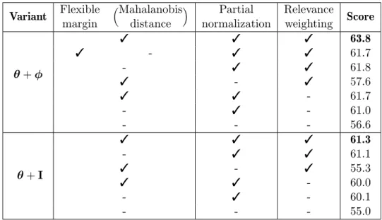
independently implemented. The generative models, marked with †, rely on stronger hypotheses as explained in Section 1.2.4. Our results are averaged over 10 runs. . . 91 2.2 Ablation study on the CUB dataset for the two variants of our model θ + ϕ and θ + I.
Results are averaged over 10 runs. . . 91 2.3 GZSL results for different ZSL models on 3 datasets. Results reported in [161] are
marked with * next to the model’s name. Other results are reported from their re-spective cited articles, except for RidgeV→S and RidgeV→S which were independently
implemented. The generative models, marked with †, rely on stronger hypotheses as explained in Section 1.2.4. Our results are averaged over 10 runs. . . 93
2.4 Intra-class and inter-class variance for several datasets. Intra-class variance is the mean squared distance between visual samples of a class and the mean of samples from this class, averaged over all classes. Inter-class variance is the mean squared distance be-tween all samples and the mean sample. . . 100 2.5 Reproduction of ZSL results from [163, 161], as measured by AU →U. “Mean” is the
mean result over 5 runs with different random initializations. “std”, “min” and “max” are the respective corresponding standard deviation minimal score and maximal score obtained over these 5 runs. . . 102 2.6 Reproduction of GZSL results from [163, 161], as measured by AU →U, AU →U and H.
We report the mean result as well as the standard deviation over 5 runs with different random initializations . . . 103 2.7 GZSL results without calibration, with calibration, and with calibration and
hyper-parameters specific to the GZSL task. Result are averaged over 5 runs. . . 105 2.8 GZSL results without calibration, and with calibration and hyper-parameters specific
to the GZSL task. Results from [161] are marked with * next to the model’s name. Results with calibration were all obtained from our independent implementation, use 10crop visual features, and are averaged over 5 runs. The generative models, marked with†, rely on stronger hypotheses as explained in Section 1.2.4. Results for our model are averaged over 10 runs. . . 108
3.1 ZSL accuracy on the large scale ImageNet dataset, for three embedding models Word2vec, GloVe and FastText. We compare the results from the proposed approaches flwiki flcust
and to the baselines wiki and clue as well as pre-trained embeddings (pt ). We use the experimental protocol from [53]. Results marked with “*” correspond to a setting close to Table 2 from Hascoet et al. [53], and are consistent with the results reported there. 119 3.2 ZSL accuracy on the smaller scale CUB dataset with unsupervised semantic embeddings.
We use the “proposed splits” from Xian et al. [163]. . . 120 3.3 ZSL accuracy on the smaller scale AwA2 dataset with unsupervised semantic
3.4 ZSL accuracy on the ImageNet dataset for different models with the flcust approach
with FastText embeddings, with distinct pairs of words (wi, wj) limited to 1 per user
(left), or without restrictions on the impact of each user (right). . . 122 3.5 ZSL performance with 100%, 50%, 25% and 10% of the initial data from the wiki and
flcust collections. Results obtained on the ImageNet dataset, with FastText embeddings. 124
3.6 Comparison of approaches on ImageNet with WordNet definitions, with the RidgeS→Vmodel.
The result marked with * corresponds to a setting similar to [53] (use of Classname with GloVe embeddings) but with a different model. . . 134 3.7 Multi-proto pred. column: the Multi-Prototype model is trained with Equation (3.14).
DeViSE is trained with the standard triplet loss similarly to Equation (3.11). Predic-tions are made with Equation (3.15), P = Q = R is cross-validated when applicable. Standard pred. column: same as leftmost column, but predictions are made with Equa-tion (3.16). P = 1 column: we fix P = Q = R = 1. P = ∞ column: all lemmas or all words from definitions are used. The results are obtained on the ImageNet dataset with WordNet definitions and lemmas, and GloVe embeddings. . . 136 3.8 Comparison of approaches on ImageNet with WordNet definitions, with the RidgeS→Vmodel.
The result marked with * corresponds to a setting similar to [53] (use of Classname with GloVe embeddings) but with a different model. . . 140 3.9 Top-k ZSL accuracy for different models, using the Classname+Defvisualness+Parent
prototypes built from FastText embeddings. Results for models marked with * are reported from [53] and employ Classname prototypes with GloVe embeddings, but make use of additional graph relations for models marked with†. . . 141 A.1 Training parameters for the different semantic embedding models. . . 167 A.2 Command lines used to train the embeddings. . . 167
1.1 A giraffe and a tiger, not necessarily in this order. . . 31 1.2 Illustration of a simple zero-shot learning (ZSL) model. In the training phase, the model
learns the relationship between visual instances and class attributes. In the prediction phase, the model estimates the presence of attributes in test images, and predicts classes from the corresponding prototypes. . . 36
2.1 t-SNE [96] visualization of 300 visual instances from the first 8 training classes of the CUB dataset. Classes least auklet (purple) and parakeet auklet (brown) are much more similar to each other than classes least auklet and laysan albatross (orange). The nestling from class laysan albatross is quite dissimilar from other samples from this class. . . . 75 2.2 Left : histogram of the raw semantic distances M as measured on the seen classes from
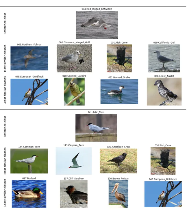
the CUB dataset, with mean distance ˆµM and standard deviation ˆσM approximately equal to 15.4 and 1.2. Right : rescaled with µM and σM set to respectively 0.5 and 0.15. 78 2.3 Most similar and least similar classes to classes “red-legged kittiwake” (top) and “arctic
tern” (bottom) from the CUB dataset, as measured by Equation (2.4). Examples for additional classes are provided in Appendix A.3. . . 79 2.4 Average norm of the projected visual features ∥θ(x)∥2 with respect to the margin M as
measured on the CUB dataset. The value ρ = 0 corresponds to no (partial) normalization. 81 2.5 Histogram (blue) of the distances to the class centerx∗c(Equation (2.12)) and associated
weights (orange) from Equation (2.17) for visual samples from class “laysan albatross” from the CUB dataset. The weights of the nestling and adult samples represented in Figure 2.1 are respectively 0.02 and 0.78. . . . 84
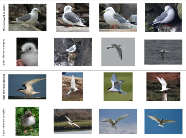
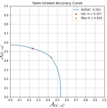
2.6 Most and least representative samples from classes “red-legged kittiwake” (top) and “arc-tic tern” (bottom) from the CUB dataset, as measured by Equation (2.17). Examples for additional classes are provided in Appendix A.3. . . 84 2.7 Seen-Unseen Accuracy Curve for the RidgeS→V model evaluated on the CUB dataset.
When γ=0, we obtain an AU →Cof 23.7 and an AS→Cof 52.8, resulting in an H of 32.7 as
in Table 2.3. When γ = +∞, only unseen classes can be predicted and AU →Cis maximal
and equal to 53.5, which corresponds to the ZSL score AU →U from Table 2.1. When
γ = −∞, only seen classes can be predicted and AS→C is maximal. The best possible
trade-off between the two occurs when both AU →C and AS→C are approximately equal
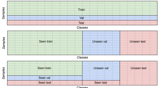
to 43.4, resulting in a maximum theoretical H of 43.4. The AUSUC is the area under the curve. . . 94 2.8 Training-validation-testing splits in different settings. Each column represents a class,
and each small rectangle a sample of this class (classes are represented as balanced in this figure, even though this is not necessarily the case). Top: standard ML split, with respect to samples. Middle: “classical” ZSL split, with respect to classes. Bottom: proposed GZSL split. . . 96 2.9 Illustration of how the regularization parameter λ of the RidgeS→V model affects the
accuracies on samples from seen and unseen classes AS→S (blue) and AU →U (red), as
measured on the test sets of CUB (left) and AwA2 (right). The optimal value for λ is not the same in a ZSL setting, where performance is measured with AU →U (red vertical
dotted line), and in a GZSL setting, where performance is measured by the harmonic mean H of AU →C and AS→C (black vertical dotted line). . . 98
2.10 Left: Illustration of the bias-variance decomposition. Right: Mean squared error of predicted attributes (averaged over attributes and samples) as a function of the reg-ularization parameter λ with the RidgeS→V model on the validation set of the AwA2
dataset. . . 99
3.1 Histogram of the most frequent words in a context window of size 4 around the word “tiger” in the Wikipedia corpus. . . 112
3.2 Ablation of manual attributes on the CUB (left) and AwA2 (right) datasets. Each time, a random subset of the attributes is selected, and the resulting ZSL score is mea-sured with the RidgeS→V model. The blue dots indicate the mean score over 10 runs
with different random attributes selected, the vertical blue bars indicate corresponding standard deviations. Best results for prototypes based on unsupervised word embed-dings are also reported for the proposed method (yellow horizontal line) and previous embeddings (red horizontal line), all with the RidgeS→V model. . . 123
3.3 (a) Distance from predicted class to correct class in the WordNet hierarchy. Correlation
ρ between ZSL accuracy and (b) distance to the closest seen class, (c) the number of
immediate unseen test class siblings, (d) the number of unseen classes closer than the closest seen class, for all 500 unseen ImageNet classes. . . 125 3.4 Graph visualization of parts of the WordNet hierarchy. Green and pink leaves are resp.
seen and unseen classes. Intermediate nodes are orange if there is no seen class among their children, and blue otherwise. Full graph is available in Figure A.7. . . 127 3.5 Australian terrier (left) and Irish terrier (right). . . 127 3.6 Top: words with highest visualness. Bottom: words with lowest visualness. The
visu-alness of a word is the inverse of the mean distance (shown in parenthesis) to the mean representation of visual features from the top 100 corresponding images from Flickr. Top 1 image with no copyright restriction is displayed. Words with the highest and lowest visualness as well as corresponding inverse visualness (the mean distance to the mean feature representations for images associated with this word) and the correspond-ing top image result with no copyright restriction from Flickr. . . 130 3.7 Inverse of the visualness (low values correspond to high visualness) for the 4059 words
from class names and WordNet definitions. . . 130 3.8 Illustration of definitions and attention scores on some test classes from ImageNet, with
the associated WordNet definitions. Left : weights from the Defvisualness approach after
softmax; the temperature is τ = 5 so differences are less pronounced than initially. Right : weights learned with the Defattention approach, with FastText embeddings. . . 131
3.9 Illustration of the word compatibilies associated with the descriptions of the top-5 can-didates with the multi-prototype method. Compatibility is displayed for words with a positive compatibility only. P = Q = R = 3 is used for training and predictions. The correct class is displayed in orange. . . 137
A.1 Top 4 most (middle) and least (bottom) similar classes to class Laysan Albatros (top). 168 A.2 Top 4 most (middle) and least (bottom) similar classes to class Least Auklet (top). . . 169 A.3 Top 4 most (middle) and least (bottom) similar classes to class Vesper Sparrow (top). 169 A.4 Top 4 most (top) and least (bottom) relevant samples for class Laysan Albatros . . . . 170 A.5 Top 4 most (top) and least (bottom) relevant samples for class Least Auklet . . . 170 A.6 Top 4 most (top) and least (bottom) relevant samples for class Vesper Sparrow . . . . 171 A.7 Overview of the full class hierarchy. Pink nodes refer to test classes, green nodes refer
to train classes, orange nodes have only test classes below them and blue nodes are other intermediate nodes. Best viewed in color with at least 600% zoom. . . 172
Computer vision is becoming of increasing importance in many scientific and industrial fields. Handwritten digits on bank checks or postal mail have been read and processed automatically for years [84, 85]. Smartphones can now be effortlessly unlocked using face recognition [134, 133]. Crop yields can be monitored from aerial and satellite images [106]. Early detection of cancer cells in medical images may soon contribute to save thousands of lives [58]. Autonomous driving promises to revolutionize mobility [27]. And many future game-changing innovations are probably just waiting to be envisioned.
Yet, giving visual abilities to a computer is not straightforward. Even something as simple for a human as differentiating pictures of cats and dogs is not straightforward to computerize. Defining precisely on a pixel-level the properties that an image must possess to represent a cat or any other high-level category proved to be an insurmountable challenge. Instead, computer vision practitioners use a completely different paradigm: rather than attempting to explicitly specify the defining features of a cat as fixed rules, they let the program learn the differences between cats and dogs from examples. This generic approach is widely known as machine learning. More specifically, virtually all the applications mentioned above rely on deep convolutional neural networks [86]. These architectures produce higher-and higher-level features, computed sequentially using kernels whose parameters are learned by the model on a large number of training examples. As an example, AlexNet [72], the architecture that won the 2012 edition of the ImageNet Large Scale Visual Recognition Challenge (ILSVRC) [132] and arguably initiated the latest deep learning revolution [83], had access to more than one million labeled images. While seemingly impressive, this amount of training data is now dwarfed by recent models [143, 16] trained on datasets with 300 million images [143].
Despite allowing unmatched performance, deep learning models’ need for data uncovers other challenges. The most obvious one is the important human annotation effort required to provide the large amount of labels necessary to train a deep model in a supervised learning setting. This may limit applications when stakeholders do not have the resources or means necessary to implement such a large investment. Furthermore, there are some classes for which it may be hard to collect hundreds or thousands of images. As an example, the saola, a critically endangered, antelope-like species from Vietnam, has only been photographed a handful of times in the wild since its discovery in 1992 [147]. More critically, the outputs of deep learning models are integrally dependent on the data used to train the model. This raises additional concerns regarding the quality and objectivity of data, as human
biases reflected in training datasets may have dire consequences [127].
Active efforts have been exerted by the research community to address this insatiable need for data. The transfer learning framework aims to transfer “knowledge” acquired by a model on a source problem onto a target problem, and thus reduce the amount of data necessary for the target problem. The main idea can be illustrated by a model trained to classify cats and dogs, and then retrained to classify tigers and wolves: its ability to identify snouts and fur patterns acquired from the source problem may also be useful in the target problem [145]. In practice in the case of convolutional networks, this often consists in re-using the weights of low-level kernels [125, 25]. A bit more specifically, the task of few-shot learning consists in designing models capable of accurately recognizing new categories after being exposed to only a few training examples, usually by heavily re-using abilities previously acquired on source problems [99, 137]. One-shot learning is the extreme application of this idea, where only a single training sample is allowed in order to assimilate new categories [39, 74].
And yet, the task of zero-shot learning aims to bring this strategy one step further. The goal of this ultimate exercise in terms of data frugality is to design models capable of recognizing objects from categories for which no training examples are provided [77, 75, 112]. The basic principle can be illustrated by the human ability to relate visual and non visual contents. For instance, someone who has never seen a single picture or illustration of a tiger – and naturally has never seen one in real life either – should still be able to recognize one instantly if they were told that a tiger is similar to a (very) big orange cat with black stripes and a white belly. Quite evidently, there needs to be some sort of semantic information similar to the “striped orange cat” description regarding the class tiger for zero-shot recognition to be possible. In this sense, zero-shot basic principles are actually quite different from few- and one-shot learning, as these tasks are usually purely visual tasks. On the other hand, zero-shot learning is by essence a multimodal task, which requires the ability to relate content from the visual modality (i.e. images) to at least one non visual modality (e.g. text, attributes...). More precisely, in this document, we consider that the term zero-shot learning refers to the design and training of a model whose goal is to classify images from unseen classes, for which no training examples are provided. Instead, training instances from strictly different seen classes can be accessed by the model during training. In addition, semantic information is provided for both seen and unseen classes.
Historically, this concept of zero-shot learning emerged more than a decade ago, with pioneering works such as the ones from Larochelle et al. [77], who first performed classification on test classes distinct from training classes, or Lampert et al. [75], who used attributes such as “black”, “brown” or “has stripes” to classify images of animal species for which no training examples were available. Around the same time, Farhadi et al. [37] likewise emphasized the relevance of predicting attributes from images in order to relate them to attributes from different classes; Palatucci et al. [112] similarly attempted to classify “unseen” words from functional magnetic resonance images (fMRI) of neural activity, using semantic representations constructed from either attributes or word co-occurrence statistics. These pioneering methods were generally fairly simple, but nevertheless led to promising results for this novel and challenging task.
This quickly sparked interest in the computer vision community, and new models and benchmark datasets were quickly introduced [129, 99, 2, 40, 138, 108]. Different settings were considered: Socher et al. [138] introduced a novelty detection mechanism, so that models could recognize both unseen and seen classes, a setting which later became known as generalized zero-shot learning [24]. Rohrbach et al. [128] popularized the transductive zero-shot learning task, in which unlabeled samples from unseen classes are available during training [42, 69]. Multi-label zero-shot recognition [98, 44], zero-shot detection [8, 124, 32] or zero-shot segmentation [19] were also proposed. Zero-shot learning was conjointly applied to other modalities, such as video and action recognition [93, 52] or natural language understanding [13, 141]. In parallel, the “deep learning revolution” gained momentum in computer vision, with better performing architectures being regularly introduced [136, 144, 55]. The use of these pre-trained networks as feature extractors [125, 25, 120] enabled zero-shot learning to benefit from these progresses [40, 108].
As a general framework aiming to drastically reduce the amount of data required to train models, zero-shot learning is arguably all the more relevant in a large scale setting. Consequently, Rohrbach et al. [129] proposed to employ 200 out of 1000 classes from ILSVRC as unseen test classes, making use of hierarchical information from WordNet to create class representations. Frome et al. [40] pushed the scale even further, by using the 1000 classes from ILSVRC as seen training classes and 20,000 additional classes from ImageNet as unseen test classes. As providing attributes for thousands of classes is impractical, scalable semantic representations are required in such a large scale setting. These representations usually take the form of word embeddings [100, 102], which consist in rich
vector representations of words capturing interesting semantic properties. The embeddings have the big advantage of typically coming from models trained on huge text corpora in an unsupervised manner, and thus of requiring close to no human annotation effort. It was thus proposed to use pre-trained word embeddings of class names as semantic representations in a large scale zero-shot learning setting [40, 138, 108].
The ability to successfully classify images in this setting could arguably be considered as the “Holy Grail” of effort-efficient approaches, as this could theoretically produce models capable of recognizing thousands of classes with close to no human annotation effort. However, in practice, performance remains modest, with reported accuracies on standard large scale benchmarks arguably too low for many practical use cases [53]. In general, performance of zero-shot learning models is unsurprisingly lower than performance of standard supervised models [164]. In addition, most zero-shot learning approaches tend to suffer from additional limitations. For instance, in the more realistic generalized zero-shot learning setting in which test classes can be either seen or unseen, many existing models tend to predict seen classes far more often than unseen classes [24, 163], which greatly decreases performance on the latter and thus the interest of using zero-shot recognition. This imbalance between seen and unseen classes is partly reduced with recent generative approaches [17, 152, 162], but this comes at the cost of more restrictive hypotheses, since contrary to other approaches, the addition of new classes often requires additional training for such models.
In this thesis, we attempt to address some of these limitations to efficient large scale zero-shot learning. We analyse existing approaches to zero-shot learning, and in particular models based on the hinge rank loss. We argue that previous models of this family implicitly make several assumptions regarding the nature of classes and training samples, and that these assumptions may not be justified in practice. In particular, these models typically consider that all classes are “equally different”, meaning that no two classes are considered closer to each other than to other classes. Previous models further assume that every training instance is representative of its corresponding class. On the contrary, we argue that this is not the case in practice, and that failing to account for these two factors may be detrimental to the performance of the model. We thus propose a model capable of taking these elements into account, with the aim of improving the robustness of the learned multi-modal relations. We also consider the performance gap between seen and unseen classes in a generalized zero-shot
learning setting. We investigate theoretical aspects of this phenomenon, and propose a simple process to reduce the difference in accuracy between instances from seen and unseen classes. Experiments are conducted to test the effectiveness of this process as well as the performance of the previously proposed model. Results confirm that the combination of both propositions enable to obtain state-of-the-art results in the tasks of classical and generalized zero-shot recognition. The proposed approach also has the advantage of enabling the effortless addition of new unseen classes to a trained model: contrary to most existing generative approaches, no additional training is required.
Keeping in mind the objective of keeping annotation efforts to a minimum, we investigate the role of semantic representations obtained in an unsupervised manner which are typically employed in a large scale setting, as this aspect is surprisingly under-studied in the current literature. We argue that generic text corpora may not be suitable to generate embeddings capturing meaningful visual properties of words, and instead propose new corpora together with a suitable pre-processing method. We conduct extensive experiments to measure the impact of this approach and explore its limitations. Nonetheless, in spite of significantly improved results enabled by our proposed method, we argue that using word embeddings of class names as semantic representations may eventually have insur-mountable limitations. We thus propose a compromise between employing unsupervised embeddings requiring absolutely no effort and laboriously providing extensive attributes, in the form of using short sentence descriptions in natural language. We propose several approaches to exploit such sentences, and eventually opt for semantic representations consisting of combinations of unsupervised representa-tions and short sentence descriprepresenta-tions. We show that this combination enables to obtain state-of-the-art results in a large scale zero-shot learning setting, while keeping the amount of human annotation effort required at a fairly reasonable level.
This manuscript is organized as follows:
• In Chapter 1, we provide a generic overview of the field of zero-shot learning for visual recognition. In particular, we introduce the different existing settings such as the generalized or transductive settings; we present the main families of approaches; and we explain how visual features and semantic representations are usually obtained. We also provide more details on tasks relevant to this document such as generalized zero-shot learning.
• In Chapter 2, we focus on identifying unjustified assumptions made by existing models and hinge rank loss models in particular, and we introduce a model taking the corresponding aspects into account. In addition, we attempt to address the gap between seen and unseen classes mentioned previously by providing theoretical insight and corresponding empirical evidence, and we propose a simple process to address this gap. We provide detailed experiments to evaluate the impact of the proposed approaches.
• In Chapter 3, we focus more specifically on the semantic representations used for large scale zero-shot learning. We collect new text corpora arguably more suitable for the creation of visually discriminative embeddings, and propose a process to train embeddings from these corpora. We also introduce several approaches to employ short sentence descriptions as semantic embeddings. We provide experimental results for these different methods.
• Finally, Chapter 3.6 provides a summary of these contributions as well as directions for future research.
At least some contributions from most parts of this document were published in different scientific venues. The publications corresponding to each part are provided in Chapter 3.6. Furthermore, the code corresponding to the experiments has most of the time been made publicly available. This information is also provided in Chapter 3.6.
Throughout this document with maybe the exception of this introduction and Section 1.1.1, we assume that the reader has working knowledge of machine learning and deep learning. In particular, we assume the reader is familiar with the – non exhaustive – concepts of a loss function, overfitting, regularization, gradient descent, back-propagation, convolutional neural networks... We refer the reader to [12] for an introduction to machine learning and to [46] for an introduction to deep learning if needed.
State-of-the-Art
Content
1.1 An introduction to zero-shot learning . . . 31 1.1.1 What is zero-shot recognition? . . . 31 1.1.2 A simple example . . . 34 1.1.3 Formal framework . . . 37 1.1.4 Zero-shot learning settings . . . 38 1.2 Standard methods . . . 42 1.2.1 Baselines . . . 42 1.2.2 Ridge regression . . . 45 1.2.3 Ranking methods . . . 51 1.2.4 Generative methods . . . 56 1.3 Visual and semantic representations . . . 62 1.3.1 Visual features . . . 62 1.3.2 Semantic representations . . . 64 1.4 Generalized zero-shot learning . . . 67
In this chapter, we provide a generic overview of the field of zero-shot learning, and particularly of the different experimental settings, the different families of methods, and the visual and semantic representations frequently employed. Importantly, although the term zero-shot learning may have several meanings, we consider in this chapter and in virtually all of this document that this refers to the task of designing a training a model whose end goal is the classification of images from classes not seen during training. This is in contrast to tasks where the end goal may be image segmentation [19], or where the entities to classify may be sentences [141], which are beyond the scope of this document. Other surveys of the field of zero-shot learning [43] or categorizations of zero-shot learning methods have been produced [161], including fairly recently [157]. However, the organisation of this section and
attempt to be fully comprehensive. As of October 2020, a query with the exact wording “zero-shot learning” in Google Scholar returns more than 5000 results, so we argue that such an endeavour is not reasonably feasible anyway.
This chapter is organized as follows: Section 1.1 provides a general public introduction to zero-shot learning (Section 1.1.1), introduces a more formal framework with a more detailed description of a simple method (sections 1.1.2 and 1.1.3), and introduces different settings such as transductive or generalized zero-shot learning. Section 1.2 provides a broad categorization of zero-shot learning models organized as baseline models (Section 1.2.1), least square regression models (Section 1.2.2), hinge rank loss models (Section 1.2.3) and generative models (Section 1.2.4). Specific details are included for several noteworthy models from each category. Section 1.3 provides information on the main types of visual features and semantic representations most frequently employed by zero-shot learning methods. Finally, Section 1.4 provides more details on the generalized zero-shot learning setting, as such details will be necessary in other chapters.
1.1
An introduction to zero-shot learning
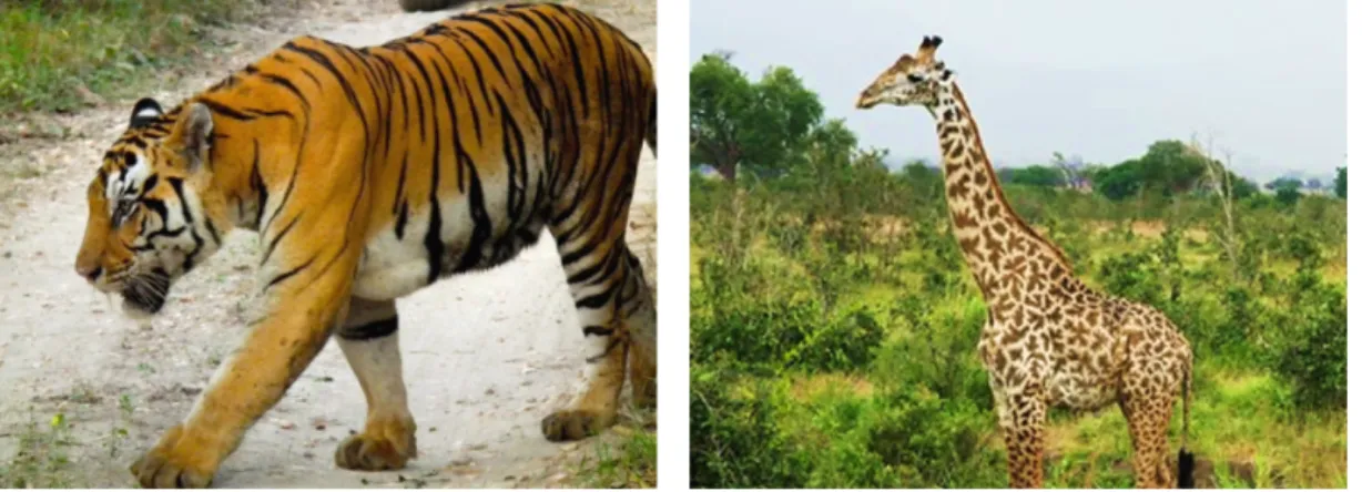
1.1.1 What is zero-shot recognition?Figure 1.1 – A giraffe and a tiger, not necessarily in this order.
The zero-shot recognition task consists in assigning the correct names to items that the entity performing the classification has never encountered before. Most humans are reasonably capable of this feat.
As an example, let’s imagine a person that has never seen a tiger in his life, neither directly nor through any indirect visual support such as books, movies or cartoons. Let’s further imagine that this person has never seen or heard of a giraffe. We give this person the following descriptions, adapted from their respective Wikipedia entries:
The tiger is the largest extant cat species. It is most recognisable for its dark vertical stripes on orange-brown fur with a lighter underside.
The giraffe’s chief distinguishing characteristics are its extremely long neck and legs, its horn-like protuberances, and its distinctive brown patches on a lighter coat.
We then proceed to show them pictures of tigers and giraffes as in Figure 1.1 and ask them to tell us which ones correspond to a tiger and which ones correspond to a giraffe. Provided this person speaks English, has previously seen other animals such as cats, understands the concepts of stripes, necks, colors and fur, is of average intelligence and is willing to cooperate, it is reasonable to expect that they will successfully be able to complete this exercise.
Notation Meaning
x a scalar
x a vector
X a matrix
xi or (x)i the ith element (scalar) of vector x
Xi,j or (X)i,j the element (scalar) at line i and column j of matrix X
ID the D × D identity matrix
0D / 1D the D-dimensional vector whose elements are all 0 / 1
diag(a) the square diagonal matrix whose diagonal
elements are the elements of vector a a2 the vector whose elements are the elements of a squared
|A| the determinant of A
A−1 the inverse of A
A⊤ the transpose matrix of A
f (·) a function returning a scalar
f (·) a function returning a vector
f (· ; w) or fw(·) a function parameterized by w
F [·] a functionnal (taking a function as input
and returning a scalar)
∥·∥p the p-norm
∥·∥2 or ∥·∥ the euclidean norm for vectors or
the Frobenius norm for matrices
⊙ the Hadamard (element-wise) product
f (a) / f (A) the element-wise application of f
on the elements of a / A 1[·] the indicator function (1 if · is true, 0 otherwise)
P (·) a discrete probability
p(·) a continuous probability density function
N (·|µ, Σ) the multivariate gaussian density function
{xk}k∈
J1,K K a set of K elements x1. . . xK
|{xk}k| the cardinal of a set
exp(·) the exponential function
log(·) the natural logarithm function
σ(·) the sigmoid function
tanh(·) the hyperbolic tangent function
[ · ]+ the function max( · , 0)
Symbol Meaning
CS the set of seen classes
CU the set of unseen classes
C the set of all classes CS∪ CU
V the visual space RD
S the semantic space RK
xn∈ RD the D-dimensional visual features of the nth image
yn∈ C the label of the nth image
sc∈ RK the K-dimensional semantic prototype of class c
tn∈ RK the prototype syn associated with (xn, yn)
X ∈ RN ×D the visual features of all N images, arranged in lines
y ∈ CN the labels associated with all N images
S ∈ RC×K the semantic prototypes of all C classes, arranged in lines T ∈ RN ×K the semantic prototypes corresponding to individual images
xtr / xte a training / testing visual instance
xcm the mth instance of class c
Dtr the training dataset ({(xn, yn)}
n∈J1,N K, {sc}c∈CS)
Dte the testing dataset
f (x, s; w) a compatibility function RD× RK → R, with parameter w
L( · ) a loss function
λΩ[f ] a regularization on f , weighted by hyper-parameter λ Table 1.2 – Frequently used notations
Abbreviation Meaning
ZSL Zero-Shot Learning
GZSL Generalized Zero-Shot Learning
CNN Convolutional Neural Network
GAN Generative Adversarial Network
VAE Variational Auto-Encoder
SVM Support Vector Machine
SGD Stochastic Gradient Descent
We can identify three main ingredients which are necessary to achieve this task:
• Things to recognize, in our case tigers and giraffes.
• Semantic information on things to recognize. For instance, the fact that tigers have stripes, giraffes have a long neck, etc.
• The ability to link the semantic information to the things to classify. This generally requires previous experience involving both visual instances and the semantic information. For example, the concept of striped fur can be learned by seeing zebras and being told the alternating black and white patterns on its back are called “stripes”.
Learning to associate the visual and semantic features with the objective to perform zero-shot recognition is usually called Zero-Shot Learning (abbreviated ZSL), although zero-shot learning and zero-shot recognition are often used interchangeably.
1.1.2 A simple example
Task and notations. We start by describing a very simple way to train a model to perform zero-shot recognition and introduce some useful notations in the process. Such notations are summarized in Table 1.2. In addition, mathematical notations used in this document are similarly summarized in Table 1.1, while frequently used abbreviations such as ZSL are summarized in Table 1.3.
The objective is to train a model to classify images belonging to categories that the model has never seen before. Such categories will be referred to as unseen classes, as opposed to seen classes, which can – and should – be used to train the model. In the previous example, tiger and giraffe would be considered unseen classes, whereas cat and for example zebra would be seen classes. Seen and unseen classes are sometimes also called respectively source and target classes. We will call the set of seen classes CS, and the set of unseen classes CU. The set of all classes is C = CS ∪ CU, with CS∩ CU = ∅.
For each class c ∈ C, semantic information is provided. For now, let us suppose that this informa-tion consists of binary attributes, for example “is orange”, “has stripes”, “has hooves” and “has a long neck”. In such a case, the semantic representation for tiger is the vector (1 1 0 0)⊤ since a tiger is – at
least partly – orange, has stripes, and does not have hooves nor a long neck1. Similarly, the semantic representation for giraffe can be (1 0 1 1)⊤. For a given class c, we call scits corresponding semantic
representation vector. Such a vector is also called the class prototype. Prototypes of all classes have the same dimension, which we call K, and represent the same attributes. More generally, the semantic information does not need to be binary attributes, and may not need to be attributes at all. More details on the most common types of prototypes are provided later in Section 1.3.2. But for now, suffice is to say that most ZSL methods can be applied as long as all classes are represented by vectors with the same characteristics (number of dimensions and meaning of each dimension).
Additionally, for each class c, a set of images {I1, . . . , IM} is available. Raw images are not always
convenient to work with, particularly in a ZSL context. For this reason, we don’t usually make use of the raw pixels themselves, but rather of a vector of high-level visual features extracted from this image. For image Ii, we write this vector xi ∈ RD, D being the fixed dimension of the visual features
space. xi is typically extracted from Ii using a pre-trained deep neural network; more details on this
process are provided in Section 1.3.1. For the sake of brevity, we will sometimes refer to xi as the ith
image, although it is not strictly speaking an image. We will also refer to xi as a visual sample, or an
instance of class c.
Zero-shot recognition is customarily achieved in two phases: a training and a testing phase. During the training phase, the model typically only has access to the semantic representations of seen classes {sc}c∈CS, and to the images (or corresponding visual features) associated with these classes. We usually write {xn}n∈J1,N K the set of N images available to the model during the training phase. yn∈ C
S refers
to the class associated with, or label, of training image xn. The full training dataset, i.e. the information
to which the model has access during the training phase, is thus Dtr= ({(xn, yn)}n∈
J1,N K, {sc}c∈CS).
During the testing phase, the model has access to the semantic representations of unseen classes {sc′}c′∈CU, and to the N′ unlabeled images belonging to unseen classes {xn′}n′∈
J1,N
′
K. We will
some-times write xtr or xte to make it explicit whether x belongs to the training (tr) or testing (te) set, if there is a possible ambiguity. The objective for the model is to make a prediction ˆyn′ ∈ CU for each test image xten′, assigning it to the most likely unseen class.
We now have novel things to recognize, semantic information regarding these things, and training 1These classes and these attributes are actually part of the Animals with Attributes dataset [76, 161], described in
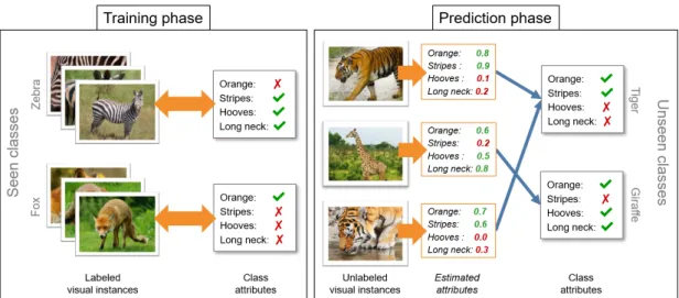
Figure 1.2 – Illustration of a simple zero-shot learning (ZSL) model. In the training phase, the model learns the relationship between visual instances and class attributes. In the prediction phase, the model estimates the presence of attributes in test images, and predicts classes from the corresponding prototypes.
data with similar semantic information associated to visual samples. All that is missing is a way to link the semantic and visual features.
A first zero-shot learning model. The following approach was first proposed in [75], and is one of the very first attempts to perform zero-shot recognition. It consists in a simple probabilistic framework, which computes the probability of presence of fixed binary attributes for a given visual input, and uses these estimated probabilities to predict the most likely unseen class corresponding to the image. Let us recall that for each class c, we have a semantic representation sc composed of binary
attributes. Although the value of the attributes may change, the attributes themselves are the same for all classes. Let’s call a1 the first of these attributes, for example “is orange”. Similarly, we will call
the other attributes a2, . . . , aK. For every training image xn, we know its class yn and have access to
the corresponding semantic attributes syn. The corresponding k
thattribute a
kof image xnis therefore
(syn)k ∈ {0, 1}.
For any attribute ak, we can thus build a labeled training set Dk = {(xn, (syn)k)}nwith the training images and corresponding labels indicating whether attribute ak is associated with each image. We
ak is present in an image x. This classifier can be a simple logistic regression2, in which case
P (ak = 1|x) = σ(w⊤kx) =
1 1 + e−w⊤kx
(1.1) where σ(·) is the sigmoid function and wk are the classifier’s parameters.
At test time, given an unlabeled test image x belonging to one of the unseen classes, a few simplifying assumptions – detailed in Section 1.2.1 – lead to predict label ˆy corresponding to the
unseen class which maximizes the probability to observe the predicted attributes:
ˆ y = argmax c∈CU K ∏︂ k=1 P (ak = (sc)k|x) (1.2)
This process is illustrated in Figure 1.2.
1.1.3 Formal framework
More generally, many ZSL methods in the literature are based on a compatibility function f : RD× RK → R assigning a “compatibility” score f(x, s) to a pair composed of a visual sample x ∈ RD and a semantic prototype s ∈ RK. Ideally, if the visual sample corresponds to the semantic description, e.g. if x is of class c and s is sc, f (x, s) should be high – and vice versa. This function may be
parameterized by a vector w or a matrix W, or by a set of parameters {wi}i. We will write fw(x, s),
f (x, s; {wi}i) or use similar notations when we need to explicitly refer to these parameters. These
parameters are generally learned using the training dataset Dtr = ({(xn, yn)}n∈
J1,N K, {sc}c∈CS) by
applying a suitable loss function L and by minimizing the total training loss Ltr over the training dataset Dtr with respect to the parameters w:
Ltr(Dtr) = 1 N N ∑︂ n=1 ∑︂ c∈CS L[(xn, yn, sc), fw] + λΩ[fw] (1.3)
where Ω[f ] is a regularization penalty based on f and weighted by the hyper-parameter λ (or in some cases by a set of hyper-parameters), which aims to reduce overfitting and thus increase the generalization abilities of the model [12].
Obtaining the global minimum of the cost in Equation (1.3) is not always possible, and sometimes not desirable. In such cases, iterative numerical optimization algorithms may be used. Examples of 2In [75], either a logistic regression or a support vector machine (SVM) classifier with Platt scaling [119] is used to
such algorithms include a standard stochastic gradient descent (SGD), AdaGrad [34], RMSProp [56] or Adam [65].
After the training phase – once “good” parameters w have been learned – and given a test image x, the predicted label ˆy can be selected among candidate testing classes based on their semantic
representations {sc}c∈CU:
ˆ
y = argmax c∈CU
fw(x, sc) (1.4)
Link with the previous example. In our previous example in Section 1.1.2, the compatibility function
f between x and s was the estimated probability to observe attributes corresponding to s given image
x, assuming independence of the K attributes and using logistic regressions to estimate probabilities. It could be written f (x, s; {wk}k) = K ∏︂ k=1 (︂ sk σ(w⊤kx) + (1 − sk)(1 − σ(w⊤kx)) )︂ (1.5)
Each of the parameters wk are learned on a training set Dk = {(xn, (syn)k)}n using a standard log loss Llog:
Llog(x, y; w) = −(︂y log(σ(w⊤x)) + (1 − y)(︂1 − log(σ(w⊤x)))︂)︂ (1.6)
wk= argmin w N ∑︂ n=1 Llog(xn, (syn)k; w) (1.7)
So the loss function L in Equation (1.3) could be written: L[(xn, yn, sc), fw] =
{︄∑︁
kLlog(xn, (sc)k; wk) if sc= syn
0 otherwise (1.8)
Although no explicit regularization is mentioned in [75], it would be straightforward to add an ℓ1 or
ℓ2 penalty to the model:
Ωℓ2[f (·, · ; {w}k)] = K ∑︂ k=1 ∥wk∥22= K ∑︂ k=1 D ∑︂ i=1 ((wk)i)2 (1.9)
Other examples of compatibility and loss functions will be studied in more details in Section 1.2. 1.1.4 Zero-shot learning settings
So far, we considered that the only information available during the training phase was (1) the class prototypes of the seen classes, and (2) labeled visual samples from these seen classes. The information
Setting Description
Information available for training
Class-inductive Prototypes from seen classes only Class-transductive Prototypes from seen and unseen classes (Instance-)inductive Instances from seen classes only
(Instance-)transductive Instances from seen classes and
(unlabeled) instances from unseen classes Candidate classes during testing
Standard supervised learning Seen classes only
(Classical) ZSL Unseen classes only
Generalized ZSL Seen and unseen classes
Table 1.4 – Summary of the main zero-shot learning settings. The classical instance-inductive, class-inductive setting is assumed to be the default setting in this document.
regarding the class prototypes of unseen classes as well as unlabeled instances from these unseen classes was only provided during the testing phase, after the model was trained. In addition, the test samples for which we made predictions could only belong to these unseen classes; we considered they could not belong to a seen class, or to a new class for which no semantic information is available.
This corresponds to the most common ZSL setting, and the one we will assume is the default in this document. However, it is important to mention that other settings may be considered, with different information being made available at different times, or with different tasks being conducted. We will simply describe briefly the other possible settings in this section. Later sections such as Section 1.4 will be entirely dedicated to some of these settings and their specificities.
1.1.4.1 Available information at training time: inductive vs. transductive settings
Class-inductive and class-transductive settings. In some settings, class prototypes of both seen and unseen classes are available during the training phase. Such a setting is referred to as a class-transductive setting by [157], as opposed to a class-inductive setting in which unseen class prototypes are only made available after the training of the model is completed. In a class-transductive setting, the prototypes of unseen classes can for example be leveraged by a generative model, which tries to synthesize images of objects from unseen classes based on their semantic description (Section 1.2.4). They can also simply be used during training to ensure that the model does not misclassify a sample from a seen class as a sample from an unseen class.
use-cases. However, this still implies that the model loses some flexibility: new classes cannot be added as seamlessly as in a class-inductive setting, in which a new class can be introduced by simply providing its semantic representation.
(Instance-)inductive and (instance-)transductive settings. Some settings are even more permissive, and consider that (unlabeled) instances of unseen classes are available during training. Such a setting is called an instance-transductive setting in [157], as opposed to an instance-inductive setting. These two settings are often simply referred to as respectively a transductive setting and an inductive setting, even though there is some ambiguity on whether the (instance-)inductive setting designates a class-inductive or a class-transductive setting. Some methods use approaches which specifically take advantage of the availability of these unlabeled images [41, 128], for example by extracting additional information on the geometry of the visual manifold [42, 165].
Even though models operating in and taking advantage of a transductive setting can often achieve better accuracy than models designed for an inductive setting, we can argue that such a setting is not suitable for many real-life use cases. With a few exceptions [90, 169], most transductive approaches consider that the actual (unlabeled) testing instances are available during the training phase, which excludes many practical applications. Even without this assumption, it is not always reasonable to expect that we will have access to unlabeled samples from many unseen classes during the testing phase. One may further argue that this is all the more unrealistic as there is some evidence that labeling even a single instance per class (in a “one-shot learning” scenario) can lead to a significant improvement in accuracy over a purely zero-shot learning scenario [164].
To summarize, a ZSL setting may be (instance-)inductive or (instance-)transductive depending on whether unlabeled instances of test classes are available during the training phase. An (instance-)inductive setting may further be class-inductive or class-transductive depending on whether semantic prototypes of unseen classes are available at training time, even though this aspect is not always explic-itly stated in the literature and an “inductive setting” may designate both. The default class-inductive, instance-inductive setting is thus the most restrictive setting, but makes the fewest assumptions on the availability of information during the different phases and is therefore the most broadly appli-cable. By default, we will consider in this document that we are operating in this class-inductive,
instance-inductive setting. This will specifically be the case for models studied in Section 1.2, with a few exceptions in the section dealing with generative models (Section 1.2.4). Information on these different settings is summarized in Table 1.4.
1.1.4.2 Use of additional information
In some settings, the available information itself can be different from the default setting. For example, in addition to the semantic prototypes, some methods make use of relations between classes defined with a graph [158, 60] or a hierarchical structure [129]. Others make use of information regarding the environment of the object, for example by detecting surrounding objects [166] or by computing co-occurence statistics using an additional multilabel dataset [98]. Other methods consider that instead of a semantic representation per class, a semantic representation per image is available, for example in the form of text descriptions [126] or human gaze information [61]. Further details on some of these settings are provided in Section 1.3.2. Although all these settings can lead to interesting alternative problems, they are mostly out of the scope of this document.
1.1.4.3 Task during the testing phase: classical vs. generalized ZSL
So far, we considered that the test instances could only belong to one of the unseen classes, and thus only these unseen classes can be predicted. However, there is generally no particular reason to assume that the seen classes we encountered during the training phase cannot be encountered again when applying and testing our model; in a real-life use case, one may legitimately want to recognize both seen and unseen classes. The setting in which testing instances may belong to both seen and unseen classes is usually called generalized zero-shot learning, abbreviated GZSL.
Even though GZSL is less restrictive than standard ZSL, it presents some specific challenges which will be detailed in Section 1.4 and are not always straightforward to address. For this reason, we consider that unless stated otherwise, we are not in a GZSL setting. We will use the term classical ZSL as opposed to generalized ZSL when we need to make this explicit.
Other even less restrictive tasks may be considered during the testing / application phase. For instance, one may want a model able to answer that a visual instance does not match either a seen nor an unseen class. Or one may want to recognize entities belonging to several categories, a setting
known as multilabel ZSL [98, 44, 88]. However, these tasks are outside the scope of this document. Similarly, there exist transductive and generalized settings [140], but we dot not aim to (and are not able to) be fully comprehensive.
1.2
Standard methods
In this section, we provide an overview of the different usual types of methods which have been developed to solve the ZSL problem. Standard methods are separated into three main categories: regression methods (Section 1.2.2), ranking methods (Section 1.2.3) and generative methods (Section 1.2.4), in addition to really simple methods which we refer to as baselines (Section 1.2.1).
This is simply one possible categorization, and different ones have been proposed in [161, 43, 157]. As with all possible categorizations, it is sometimes not so clear which category best fits a given method; but overall, we think this choice is well-suited to give a general overview of the field. We would also like to emphasize that sometimes, methods described here are slightly different from their initial formulation in the original articles. This is done for the sake of brevity and simplicity; the aim is to give a general overview of the types of methods, their strengths, weaknesses and underlying hypotheses, not to dive deep in very specific implementation details. We usually try to disclose it explicitly when what is described is different from the cited article, and refer the reader to the original publications for further details.
Experimental results on standard ZSL benchmark datasets (presented in Appendix A.1) are avail-able in Tavail-able 2.5 for several methods of each category, originating from the reference comparison from Xian et al. [161] as well as from our independent reproduction of some of these results.
1.2.1 Baselines
This section describes very simple methods, which were usually proposed early in ZSL history. These methods have the advantage of being easy to implement and requiring very little computing power – or at least, no more than regular supervised classification. Some of them even enable to directly adapt a standard supervised classifier to a ZSL setting. However, their performance is usually quite low compared to more advanced methods.
We already encountered the Direct Attribute Prediction or DAP [75] approach in Section 1.1.2. Recall that this method simply consists in training K standard classifiers which provide the prob-ability P (ak|x) that attribute ak is present in visual input x. At test time, we predict the class c
which maximizes the probability to have attributes corresponding to its class prototype sc
(Equa-tion (1.2)). We now provide some addi(Equa-tional informa(Equa-tion regarding the underlying assump(Equa-tions which led to Equation (1.2).
Ideally, we would like to be able to estimate the conditional probability P (c|x) that a visual instance x belong to class c. For a given test image x, this would lead to predict label ˆy such that
ˆ
y = argmax c∈CU
P (c|x) (1.10)
From the sum and product rules of probability,
P (c|x) = ∑︂
a∈{0,1}K
P (c|a)P (a|x) (1.11)
From Bayes’ theorem,
P (c|a) = P (a|c)P (c)
P (a) (1.12)
Assuming deterministic attributes a = sc given the class c, P (a|c) = 1[a = sc] =
{︄
1 if a = sc
0 otherwise (1.13)
From equations (1.12) and (1.13),
P (c|a) = ⎧ ⎨ ⎩ P (c) P (a=sc) if a = sc 0 otherwise (1.14)
Which means we only keep one term in the sum in Equation (1.11)
P (c|x) = P (c|a = sc)P (a = sc|x) =
P (c) P (a = sc)
P (a = sc|x) (1.15)
If we further assume identical class priors P (c) and uniform attribute priors3 P (ak) = 12, the only
non-constant term in Equation (1.15) is P (a = sc|x). Finally, assuming independence of attributes, P (a|x) = K ∏︂ k=1 P (ak|x) (1.16) 3
The authors of [75] also suggest to compute attribute priors P (a) by assuming independent attributes and estimating the probability of each attribute using the training dataset, but indicate that experimental results of both approaches are similar.


![Figure 2.1 – t-SNE [96] visualization of 300 visual instances from the first 8 training classes of the CUB dataset](https://thumb-eu.123doks.com/thumbv2/123doknet/14722767.751476/76.892.277.628.198.548/figure-sne-visualization-visual-instances-training-classes-dataset.webp)