READ THESE TERMS AND CONDITIONS CAREFULLY BEFORE USING THIS WEBSITE. https://nrc-publications.canada.ca/eng/copyright
Vous avez des questions? Nous pouvons vous aider. Pour communiquer directement avec un auteur, consultez la première page de la revue dans laquelle son article a été publié afin de trouver ses coordonnées. Si vous n’arrivez pas à les repérer, communiquez avec nous à [email protected].
Questions? Contact the NRC Publications Archive team at
[email protected]. If you wish to email the authors directly, please see the first page of the publication for their contact information.
NRC Publications Archive
Archives des publications du CNRC
This publication could be one of several versions: author’s original, accepted manuscript or the publisher’s version. / La version de cette publication peut être l’une des suivantes : la version prépublication de l’auteur, la version acceptée du manuscrit ou la version de l’éditeur.
Access and use of this website and the material on it are subject to the Terms and Conditions set forth at
Three-dimensional numerical simulation of injection moulding
Ilinca, Florin; Hétu, Jean-François
https://publications-cnrc.canada.ca/fra/droits
L’accès à ce site Web et l’utilisation de son contenu sont assujettis aux conditions présentées dans le site LISEZ CES CONDITIONS ATTENTIVEMENT AVANT D’UTILISER CE SITE WEB.
NRC Publications Record / Notice d'Archives des publications de CNRC:
https://nrc-publications.canada.ca/eng/view/object/?id=aec439a4-8cda-4929-9e2a-9bf93e70897e
https://publications-cnrc.canada.ca/fra/voir/objet/?id=aec439a4-8cda-4929-9e2a-9bf93e70897e
0
Three-Dimensional Numerical Simulation of
Injection Moulding
Florin Ilinca and Jean-Franc¸ois H´etu
National Research Council, Industrial Materials Institute Canada
1. Introduction
Injection moulding of polymeric materials is an important manufacturing process used to produce cost effective parts for a large number of industries. Very often, moulded parts must satisfy stringent quality requirements in terms of mechanical behaviour and dimensional char-acteristics. Numerical simulations are cost effective and provide quick solutions, thus being an inevitable tool for the design and evaluation of the processing parameters. Numerical investi-gations are able to estimate aspects of the physical model which otherwise would be difficult to quantify. What if? tests give information on the effect of process parameters on the final part and provide setup conditions to obtain the optimal process and final part characteristics. The injection moulding cycle can be described as being formed by three main stages: filling, packing-holding and cooling. During the initial filling stage, when the molten polymer fills the cavity, compressibility effects are small and the flow is usually considered incompress-ible. During this phase, non-isothermal effects are important, even if they are concentrated in boundary layers close to the mould-cavity interface. Once the entire cavity is filled, the pro-cess enters the packing-holding stage during which a much larger pressure is applied on the material. At this point a compression occurs and the solution behaviour is driven by the poly-mer compressibility. The compression phase is very short but results in dramatic changes on the nature of the polymer flow in the cavity. Velocities may take values comparable with those during the filling stage, while the pressure increase propagates into the entire cavity. As soon as the pressure reaches its maximum value, the velocity amplitude falls. It is the beginning of the holding stage during which compressibility effects are still important. The inflow of material must compensate for the decrease of the specific volume from cooling. The polymer in the gate then freezes and the mass of polymer in the cavity is set. The physics during the remaining cooling phase are modeled by the energy and state equations.
Co-injection moulding involves injection of skin and core polymer melt into a mould cav-ity such as the core material is embedded within the solidified layers of the skin material. The process has the potential of providing optimal properties of the moulded part by using a proper combination of the skin and core materials. It may also reduce part weight, part cost, injection pressure, residual stresses and warpage when comparing with the traditional single material injection moulding. Co-injection moulding popularity increased over the last years as recent developments in machines, materials and design concepts made the process more flexible and useful. In gas-assisted injection moulding, gas is injected into the cavity in the place of a second polymer melt. Gas-assisted injection demands lower injection-packing pressure, smaller cooling times and less moulding material resulting in smaller part weight.
Gas-assisted moulded parts present more uniform properties, reduced shrinkage, warpage and residual stresses. Therefore, better final products are produced at lower costs.
A faithful model and numerical simulation of the material behaviour during injection is ex-tremely important in order to predict with confidence the characteristics of the final prod-uct. Most of the work done to simulate the injection moulding process was performed by us-ing the Hele-Shaw approximation (Kamal et el., 1975; Hieber & Shen, 1980; Chen & Liu, 1994; Chen & Hsu, 1995; Chen et al., 1995; Han & Im, 1997; Gao et al., 1997; Schlatter et al., 1999). Such approach is unable to predict fountain flow, transverse pressure gradients, and sim-plifies the modeling near corners, bifurcations and changes in the part thickness. In recent years there is increased interest in the 3D modeling for an accurate representation of the ma-terial behaviour (H´etu et al., 1998; Ilinca & H´etu, 2001; Ilinca et al., 2002; Kim & Turng, 2004; Polynkin et el., 2005). This chapter presents a full 3D numerical approach to solve the injec-tion moulding process. The methodology is perfectly well suited for three-dimensional parts for which simplifying lubrication hypothesis are inappropriate, for modeling multi-material injection or processes presenting jetting and folding of the material inside the cavity. In ad-dition to traad-ditional injection moulding applications, examples are shown for the simulation of gas-assisted injection moulding, co-injection moulding and injection moulding of metal-lic powders. Numerical solutions of the transient, three-dimensional, free surface flow and heat transfer equations describing the material behaviour during injection are obtained by a stabilized finite element method on unstructured grids and compared with experimental data.
2. Numerical Modelling 2.1 Assumptions
The constitutive equations represent the thermal and mechanical behaviour of isotropic amor-phous polymers during the filling stage of the injection moulding process. We resume here the main considerations behind the choice of model equations described in this section. The maximum pressure drop encountered during the filling of most plastic parts is about 106to 107Pa. Considering that the compressibility coefficient of most polymer melts is of the or-der of 10−9Pa−1, one can conclude that compressibility effects can be neglected. During the filling stage the polymer melt is thus considered incompressible. Second, the mechanical be-haviour of an amorphous polymer in shear dominated flows (such as in injection moulding and co-injection) can be described reasonably well by a generalized Newtonian fluid model. This assumption has been validated numerically by (Baaijens & Douven, 1991) who showed that flow kinematics predicted by viscoelastic approach do not significantly differs from the one obtained using a generalized Newtonian approach. This is also in agreement with exper-imental observations of (Janeschitz-Kriegl, 1983) and (Wimberger-Friedl & Janeschitz-Kriegl, 1988).
Polymer melts have a surface tension σ between 20 and 50mN/m (Wu, 1991) and viscosities are of the order of 103Pa·s. Velocities at the interface are of the order of 0.02m/s leading to a Capillary number Ca=ηV/σ of the order of O(103). Similar dimensional analysis leads
to Reynolds numbers (ratio of inertia to viscous forces) in the range of 10−4to 10−2. One can conclude that viscous forces dominate and that both inertia and surface tensions can be neglected in the momentum equation. Meanwhile, given the small thermal conductivity of polymers, the Peclet number takes very large values, in the range of 103to 105, and the inertia has to be taken into account in the energy equation.
2.2 Governing equations
The equations governing the incompressible melt flow are the Stokes and continuity equations
0 = −∇p+ ∇ · [2η ˙γ(u)], (1)
−∇ ·u = 0, (2)
where ˙γ(u) = (∇u+ ∇uT
)/2 is the strain rate tensor. Heat transfer is modeled by the energy equation:
ρcpµ ∂T
∂t +u· ∇T 
= ∇ · (k∇T) +2η ˙γ2. (3)
In the above equations, t, u, p, T, ρ, η, cp and k denote time, velocity vector, pressure,
tem-perature, density, viscosity, specific heat and thermal conductivity respectively. During the packing phase the compressibility of the polymer should be taken into account. The set of equations in this case includes the state equation as described in (Ilinca & H´etu, 2001). 2.3 Front tracking method
The position of the polymer/air and skin/core polymer interfaces is tracked using a level-set method (Ilinca & H´etu, 2002). The approach defines smooth functions Fi such that the
critical value Fcrepresents the position of the interface. We consider i=1 for the polymer/air
interface and i=2 for the skin/core interface. A front tracking value greater than Fcdenotes
a region filled by the respective polymer, while a smaller than Fc value corresponds to an
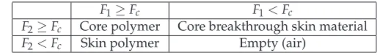
unfilled region. For co-injection and gas-assisted injection two interfaces are present and the various combinations are summarized in Table 1. The front tracking technique identifies the skin, core and empty regions. Core breakthrough is also predicted.
F1≥Fc F1<Fc
F2≥Fc Core polymer Core breakthrough skin material
F2<Fc Skin polymer Empty (air)
Table 1. Definition of filled (skin/core) and empty regions for co-injection
At each time step the level-set functions tracking the polymer/air and skin/core interfaces are obtained by solving pure advection equations using the velocity field provided by the solution of the momentum-continuity equations:
∂Fi
∂t +u· ∇Fi=0 (4)
2.4 Boundary conditions
Appropriate boundary conditions complete the statement of the problem. On the entry sec-tion both velocity and temperature are imposed. Filling is performed at constant flow rate as given by the velocity of the screw. Co-injection is performed using different barrel/screw plasticizing units, therefore the injection speed and temperature may be different for the skin and core materials. A free boundary condition is imposed on the unfilled part of the cavity walls allowing for the formation of the typical fountain flow, whereas no-slip boundary con-ditions are imposed on the filled part of the boundary. When the cavity is completely filled, the simulation stops as the no-slip boundary condition cannot allow more material to enter the cavity. The heat transfer between the cavity and the mould is given by
where hcis a surface heat transfer coefficient and Tmould is the mould temperature. For the
front tracking function, homogeneous Neumann boundary conditions are considered on all boundaries, except for the entry where Dirichlet conditions are imposed. Entry values change in time and indicate whether skin or core polymers are injected.
3. Finite element solution procedure
Model equations are discretized in time using a first order implicit Euler scheme. Linear continuous shape functions are used for all variables. At each time step, the global system of equations is solved in a partly segregated manner. The solution algorithm solves separately the systems of equations as follows:
For time smaller than the injection time:
1. Solve the incompressible momentum-continuity equations (u−p). 2. Solve the energy equation (T).
3. Solve the front tracking equation F1 (polymer/air interface) if
skin material is injected, or equations (F1, F2) if core material is
injected.
Check convergence. If converged goto the next time step, otherwise repeat steps 1 to 3.
Steps 1 to 3 are solved using the last known values of the dependent variables and iterations are made to obtain converged solutions of the coupled system of equations. The finite element formulations of the equations are discussed hereafter.
3.1 Momentum-continuity equations
The Stokes equations (1) and (2) are solved using a Galerkin Least-Squares (GLS) method (Franca & Frey, 1992). This method contains an additional pressure stabilization term compared with the standard Galerkin method. In such a way, the use of linear ele-ments for both the velocity and pressure is permitted. The GLS variational formulation of the momentum-continuity equations is:
Z Ω2η ˙γ( u): ˙γ(v)dΩ− Z Ωp∇ · vdΩ+ Z Ω∇ · uqdΩ +
∑
K Z ΩK{∇p− ∇ · [2η ˙γ( u)]} ·τu∇qdΩ K=0 (6)where v and q are velocity and pressure test functions respectively. The stabilization parame-ter τuis defined as:
τu = mkh
2
K
4η (7)
where hK is the size of the element K and mkis a coefficient commonly considered 1/3 for
linear elements. 3.2 Energy equation
For polymers, the Prandtl number takes large values. Therefore, during the filling, the en-ergy equation is dominated by the convection. However, cooling generated by the heat lost
through walls, coupled with a low material diffusivity, generates high temperature gradients in direction normal to the wall. The solution algorithm must correctly represents both advec-tive and diffusive mechanism. Here a GLS/GGLS method is used to solve for the temperature. The GLS (Franca & Frey, 1992) term stabilizes the convection, whereas the GGLS contribu-tion (Franca & Dutra do Carmo, 1989) deals with the presence of sharp boundary layers. The GLS/GGLS formulation of equation (3) is:
Z Ωρcp µ T−T0 ∆t +u· ∇T ¶ wdΩ+ Z Ωk∇T· ∇wdΩ− Z Ω2η ˙γ 2wdΩ +
∑
K Z ΩK · ρcpµ T−∆tT0+u· ∇T ¶ − ∇ · (k∇T) −2η ˙γ2 ¸ τTρcpu· ∇wdΩK (8) +∑
K Z ΩK∇ · ρcpµ T−T0 ∆t +u· ∇T ¶ − ∇ · (k∇T) −2η ˙γ2 ¸ τ∇∇wdΩK = Z Γmouldhc(T−Tmould)wdΓNote that the stabilization terms are integrated only over the element interiors. The stabiliza-tion parameter τTis defined as in (Ilinca et al., 2000):
τT = µ2ρc p ∆t ¶2 + µ2ρc p|u| hK ¶2 + Ã 4k mkh2K !2 −1/2 (9) The definition of the stabilization parameter τ∇, as from reference (Franca & Dutra do Carmo,
1989), is: τ∇=h 2 K 6 ξ (10) where ξ = cosh( √ 6α) +2 cosh(√6α) −1− 1 α (11) α = (ρcp/∆t)hK 2 6k (12)
3.3 Front tracking equations
The front tracking equations are discretized using an SUPG finite element method. SUPG provides smooth solutions when the convective part of the equation is dominant, as is in the present case. The variational formulation is given by
Z Ω µ ∂F ∂t +u· ∇F ¶ vdΩ+
∑
K Z ΩK µ ∂F ∂t +u· ∇F ¶ τF(u· ∇v)dΩK=0. (13)In the absence of diffusion the stabilization coefficient τFis defined as
τF=
hK
2|u|. (14)
The front tracking functions are discretized using linear elements. They are reinitialized after each time step to insure mass conservation of the skin and core polymers (Ilinca & H´etu, 2002).
4. Numerical applications
4.1 Filling and post-filling analysis of a plate
The first application is the simulation of the filling and post-filling stages of a polystyrene part (Ilinca & H´etu, 2001). The cavity is a rectangular plate (76.2mm by 38.1mm) of uniform thickness (either 2.54mm or 1.76mm) as shown in Figure 1.
Figure 1. Geometry of the cavity and location of control points P1, P2 and P3
This problem was the object of a numerical and experimental investigation in (Chiang et al., 1991a;b). The problem was also simulated numerically using the Hele-Shaw model by Chen & Liu (1994) and by Han & Im (1997). Conditions for numerical simulations followed those used by (Chiang et al., 1991b). The parameters were varied in order to evaluate their influence on the numerical results. Tests were performed using different values for the pack-ing pressure, cavity thickness, melt temperature and mould temperature. The computational conditions are summarized in Table 2. Experimental data at point P1 were used as inlet condi-tions for the numerical simulation. Material properties for the numerical simulation are given in (Ilinca & H´etu, 2001). The heat transfer coefficient used on the cavity-mould interface is hc=2000W/m2·0C.
Condition Case 1 Case 2 Case 3 Case 4 Case 5
Cavity thickness(mm) 2.54 2.54 2.54 1.76 1.76
Melt temperature(0C) 200 200 230 200 200
Fill time(s) 0.69 0.69 0.69 0.48 0.48
Hydraulic hold pressure(MPa) 6.9 3.45 6.9 6.9 6.9
Holding time(s) >15 >15 >15 >15 >15
Mould temperature(0C) 32 32 32 32 60
Table 2. Processing conditions for the rectangular plate
Pressure solutions at points P2 and P3 are presented in Figure 2. Comparison is made for all cases with the experimental and numerical data of Chiang et al. (1991b). Case 1 is used as a reference. In case 2 the packing pressure is reduced to half the reference value and the results are presented in Figure 2(b). For this case, the pressure decreases at the same rate as for case 1 (Figure 2(a)) but because of the smaller packing pressure, it falls to zero earlier in time and therefore at higher temperature. The net result will be that the final shrinkage of the part will be more important when the packing pressure is smaller.
0 5 10 15 20 25 30 35 40 45 50 0 2 4 6 8 10 Pressure (MPa) Time (sec.) Experiment - P1 Experiment - P2 Experiment - P3 Chiang et al. - P1 Chiang et al. - P2 Chiang et al. - P3 Present - P1 Present - P2 Present - P3 (a) Case 1 0 5 10 15 20 0 2 4 6 8 10 Pressure (MPa) Time (sec.) Experiment - P1 Experiment - P2 Experiment - P3 Chiang et al. - P1 Chiang et al. - P2 Chiang et al. - P3 Present - P1 Present - P2 Present - P3 (b) Case 2 0 10 20 30 40 50 60 0 2 4 6 8 10 Pressure (MPa) Time (sec.) Experiment - P1 Experiment - P2 Experiment - P3 Chiang et al. - P1 Chiang et al. - P2 Chiang et al. - P3 Present - P1 Present - P2 Present - P3 (c) Case 3 0 5 10 15 20 25 30 35 40 45 50 0 0.5 1 1.5 2 2.5 3 3.5 4 Pressure (MPa) Time (sec.) Experiment - P1 Experiment - P2 Experiment - P3 Chiang et al. - P1 Chiang et al. - P2 Chiang et al. - P3 Present - P1 Present - P2 Present - P3 (d) Case 4 0 5 10 15 20 25 30 35 40 45 50 0 0.5 1 1.5 2 2.5 3 3.5 4 Pressure (MPa) Time (sec.) Experiment - P1 Experiment - P2 Experiment - P3 Chiang et al. - P1 Chiang et al. - P2 Chiang et al. - P3 Present - P1 Present - P2 Present - P3 (e) Case 5
Figure 2. Pressure traces at control points P1, P2 and P3
Figure 2(c) shows the results for case 3 for which the melt temperature was increased to 2300C. The 3D solution is almost superimposed over the experimental data and the results of Chiang et al. (1991b). Because of the higher melt temperature, the polymer is less viscous than for case 1. The pressure decreases then at a smaller rate. Note that for point P1 the max-imum pressure is about 5MPa greater than for case 1. Increasing the melt temperature has a comparable effect as increasing the packing pressure.
Conditions of case 4 correspond to a thinner cavity. Pressure traces for this case are presented in Figure 2(d). The time taken by the melt temperature to decrease below the no-flow temper-ature is reduced from about 10s on the thicker plate to less than 4s on the thinner plate. The
numerical results are closer to the experimental data during the first two seconds of packing and larger differences are apparent on the later stage of the holding phase.
Simulation for case 5 (Figure 2(e)) reproduces the conditions of case 4 but with the mould tem-perature increased from 320C to 600C. Because of the lower cooling rate the pressure decreases more slowly. A good agreement is observed between experimental measurements, 2.5D nu-merical results (Chiang et al., 1991b) and present 3D predictions. We may conclude that the present numerical approach performs well and produces prediction in good agreement with experiments.
4.2 Co-injection of a center gated rectangular plate
For this application the mould cavity is a centrally gated rectangular plate with dimensions of 76x164x7mm. Experimental trials were carried out in a 150-ton Engel co-injection machine (Ilinca et al., 2006). The horizontal and vertical barrel/screw plasticizing units are used to feed the skin and core materials, respectively, to the co-injection head. The materials are injected sequentially in the mould through a single nozzle equipped with a check valve, which controls the amount of material entering the mould. A given percentage of the skin material is first injected in the cavity, followed by the injection of the core material. The material used for both skin and core is an injection grade polycarbonate Caliber 200-14 supplied by The Dow Chemical Company. Numerical results for the same part injected with and ABS polymer are reported in (Ilinca & H´etu, 2002) and (Ilinca & H´etu, 2003). For visualization purposes, a red pigment is added to the core material. The polymer viscosity is modeled with the Cross-WLF model: η(T, ˙γ, p) = η0(T, p) 1+µ η0(T, p)|˙γ| τ∗ ¶1−n. (15) η0(T, p) =D1exp · − A1(T−T∗) A2+ (T−T∗) ¸ , (16) where T∗(p) =D2+D3p, (17) A2(p) =A˜2+D3p. (18)
The rate of deformation|˙γ|is computed from the strain rate tensor as|˙γ| =√2 ˙γ : ˙γ . Model constants used for the numerical simulation are summarized in Table 3. Density, specific heat and thermal conductivity were considered constant, equal to 1162 kg/m3, 2000 J/(kg·0C),
and 0.25W/(m·0C)respectively.
Model constant Value
n; τ∗(Pa) 0.18; 5.766·105
D1(Pa·s); D2(0C); D3(0C/Pa) 3.46·106; 175.0; 0.0
A1; ˜A2(0C) 11.59; 33.98
Table 3. Cross-WLF model constants for PC200
Numerical solutions were obtained on a mesh having 44,850 nodes and 199,440 tetrahedral elements. Given the segregated nature of the solution algorithm, the maximum CFL number at the melt/air interface is limited to unity, and a typical solution needs about 150 time steps for the filling period. Computations were carried out for different skin/core ratio, skin/core
injection temperatures and skin/core injection speeds and the results were compared with the moulded parts. Process conditions and simulation results are summarized in Table III. The temperature of the injected melt was set at either 3000C or 2500C, while the mould temperature
was set at 900C. Screw speed was considered either 20mm/s or 50mm/s. At the lower injection speed, filling of the plate takes 3.5s, while at the faster speed it takes 1.4s. The reference case has a skin/core ratio of 80/20 and the same injection temperature (3000C) and injection speed (20mm/s) for both skin and core.
Case Skin/core ratio, vol.% Skin/core inj. speed, mm/s Skin/core temperature, 0C Delay time, s Core Length/Width, mm Ref. 80/20 20/20 300/300 0 47.2/30.0 A A(1): 90/10 A(2): 70/30 A(3): 60/40 20/20 300/300 0 29.2/23.4 61.2/32.8 72.9/30.0 B 80/20 B(1): 20/50 B(2): 50/20 B(3): 50/50 300/300 0 46.7/29.8 45.0/29.6 44.3/29.4 C 80/20 20/20 C(1): 300/250 C(2): 250/300 C(3): 250/250 0 44.8/30.4 51.8/28.9 48.4/29.7 D 80/20 20/20 300/300 D(1): 1 D(2): 2 D(3): 4 50.5/30.1 52.3/30.3 56.0/30.6 Table 4. Operating conditions and simulation results
Figure 3 compares the moulded part with the 3D solution for the reference case. Front view and isometric view are shown. The skin polymer is plotted in transparency in order to allow for the core to be visible. The core material advances more rapidly in the direction correspond-ing to the plate length. Because the plate fills first in the width, the core penetrates less in this direction. The 3D solution of the co-injection process is able to predict the core shape in all directions. Most important, the residual skin thickness is computed and critical regions can be identified. In this case thin polymer skin is predicted in the region of the gate. The hot polymer is directed into the opposite wall and the skin thickness is very small at this location. Far from the center, the core polymer penetrates by the mid-plane and the skin thickness is almost the same on top and bottom of the part.
(c) Front view (d) Isometric view
Figure 3. Experimental (top) and simulated (bottom) results for the reference case
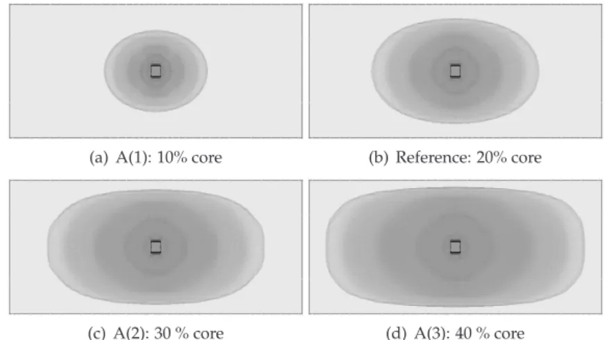
Figure 4 illustrates the change in the solution when the ratio skin/core ratio varies from 90/10 to 60/40. As more core material is injected in the cavity the core penetrates deeper inside the skin. Core penetration changes mostly in the length of the plate as the filling during core injection occurs mostly in this direction.
(a) A(1): 10% core (b) Reference: 20% core
(c) A(2): 30 % core (d) A(3): 40 % core
Figure 4. Numerical solutions for different ratios skin/core polymers
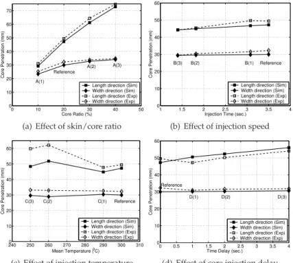
Experimental and numerical core penetration in length and width directions are compared in Figure 5. The effect of changing the skin/core ratio, the injection speed, the injection tem-perature and the core injection delay is investigated. As expected, Figure 5(a) indicates that a deeper core penetration is observed for a higher ratio core/skin materials. The effect of the injection speed is shown in Figure 5(b). By increasing the injection speed the temperature
of the polymer increases because of the shear heating and also because of the smaller cool-ing time. The net effect is that a faster fillcool-ing (i.e. higher temperature) determines a higher core thickness and therefore a shorter core penetration length. A similar effect is observed when the skin/core temperature is varied (Figure 5(c)). The mean injection temperature is computed by using 80% of the skin value and 20% of the core value. A lower temperature determines a thinner core (thicker skin) and hence a deeper core penetration. Note however that changes in skin and core temperature have opposite effects. A lower core temperature determines a higher viscosity core. Therefore, the core is thicker and the penetration length is shorter. Meanwhile, lower skin temperature determines a thicker skin and therefore deeper core penetration. Changing the core injection delay (Figure 5(d)) has a similar effect on the solution. Increasing the delay is equivalent to a lower skin temperature and hence deeper core penetration. 0 10 20 30 40 50 0 10 20 30 40 50 60 70 Reference A(1) A(2) A(3) Core Ratio (%) Core Penetration (mm)
Length direction (Sim) Width direction (Sim) Length direction (Exp) Width direction (Exp)
(a) Effect of skin/core ratio
1 1.5 2 2.5 3 3.5 4 0 10 20 30 40 50 60 Reference B(3) B(2) B(1)
Injection Time (sec.)
Core Penetration (mm)
Length direction (Sim) Width direction (Sim) Length direction (Exp) Width direction (Exp)
(b) Effect of injection speed
240 250 260 270 280 290 300 310 0 10 20 30 40 50 60 Reference C(3) C(2) C(1) Mean Temperature (0C) Core Penetration (mm)
Length direction (Sim) Width direction (Sim) Length direction (Exp) Width direction (Exp)
(c) Effect of injection temperature
0 0.5 1 1.5 2 2.5 3 3.5 4 0 10 20 30 40 50 60 Reference D(1) D(2) D(3)
Time Delay (sec.)
Core Penetration (mm)
Length direction (Sim) Width direction (Sim) Length direction (Exp) Width direction (Exp)
(d) Effect of core injection delay
Figure 5. Comparison of numerical and experimental core penetration
This results indicate a good agreement between experiment and simulation except for cases C(2) and C(3) which present core instability in the experiment. Both numerical simulation and experiment indicate that core penetration increases at longer filling times (Figure 5(b)), at higher core temperature (reference case compared with C(1) and C(2) compared with C(3)), at smaller skin temperature (reference case compared with C(2) and C(1) compared with C(3)), and at larger core injection delay (Figure 5(d)).
4.3 Gas-assisted injection of a thin plate with a flow channel
We consider here the gas-assisted injection of a rectangular plate with a flow channel on the longitudinal axis. This problem was the object of an experimental and numerical study by Gao et al. (1997). The moulded plate is 100mm wide, 384mm long and 2.5mm thick. The channel present along the centerline of the part is 325mm long, 6mm wide and 9mm deep. Material properties correspond to a high density polyethylene (HDPE). The viscosity depen-dence upon the shear rate and temperature is described by the modified Carreau-WLF model (Ilinca & H´etu, 2003):
η= η0At (1+λAt˙γ)n (19) ln(At) = 8.81(Tre f−Ts) 101.6+Tre f−Ts − 8.81(T−Ts) 101.6+T−Ts (20)
Material properties and viscosity model constants are given in Table 5. Density, ρ(kg/m3) 850.0
Specific heat, cp(J/kg/K) 4000.0
Thermal conductivity, k(W/m/K) 0.35 Zero shear rate viscosity, η0(Pa·s) 501.97
Relaxation time, λ(s) 0.00422
Power law index, n 0.698
Reference temperature, Tre f(0C) 232.3
Standard temperature, Ts(0C) -66.0
No flow temperature,(0C) 133.0
Table 5. Material properties for HDPE
Computations were done in order to quantify the solution dependence on various parameters as melt temperature, mould temperature, gas pressure, polymer/gas volume ratio, and gas injection delay. Numerical simulations for the same conditions but using a Cross-WLF vis-cosity model are given in (Ilinca & H´etu, 2002). The computational parameters, namely melt temperature, mould temperature, gas pressure, and gas volume, are summarized in Table 6. For each case, three series of computations were performed: (a) gas injected with no delay, (b) with one-second delay, and (c) with four seconds delay, respectively. For the given poly-mer injection speed, complete filling of the part would take 1 second. The cavity/mould heat transfer coefficient was taken hc=4000W/(m2·0C). The results for the gas injection time and
the length of the gas core are also listed in Table 6.
Case A is considered as a reference on which the other cases are compared. This way, the effect of different parameters on the solution behaviour is quantified. Figure 6 shows the solution at the end of the gas injection for case A. The plot was made in transparency in order to make visible the gas region inside. Gas corresponds to the darkest region and mainly follows the central channel. When gas injection is delayed, the cooling of the plate is such that the gas does not penetrate laterally in the thin plate region. Therefore, gas penetration in the flow leader is more profound. The length of the gas core is 42% longer when gas injection is delayed by four seconds than with no delay. The gas injection time is also affected. When part temperature decreases, the viscosity increases, causing a slower polymer flow. For a gas delay time of four seconds, the gas injection time increases by a factor of almost three compared to the case without delay time. For case B, the melt temperature is increased to 2700C. The polymer
Case Tmelt
(0C) T(mould0C) (MPapgas) Gas vol.% delayGas inj.(s) timeGas inj.(s) lengthGas core(mm)
A 240 35 17.25 8 A(1): 0 A(2): 1 A(3): 4 0.48 0.68 1.22 223.6 255.7 316.8 B 270 35 17.25 8 B(1): 0 B(2): 1 B(3): 4 0.36 0.51 0.92 220.4 252.2 315.0 C 240 75 17.25 8 C(1): 0 C(2): 1 C(3): 4 0.43 0.57 0.86 207.3 233.2 268.0 D 240 35 34.5 8 D(1): 0 D(2): 1 D(3): 4 0.17 0.25 0.45 217.7 251.5 311.5 E 240 35 17.25 10 E(1): 0 E(2): 1 E(3): 4 0.51 0.69 1.13 279.2 316.5 363.2∗ Table 6. Operating conditions and simulation results (∗indicates gas fingering)
being at higher temperature becomes less viscous. Therefore, the gas penetrates more in the thin regions of the plate. Results listed in Table 6 indicate that melt temperature influences less the length of the gas core but has larger impact on the gas penetration time. Meanwhile, when increasing the mould temperature (case C) the time injection delay exhibits little changes, while the length of the gas core varies more significantly. The explanation of this behaviour is that gas injection time is determined by the core polymer viscosity, which depends on the melt temperature. The length of the gas core depends on the skin polymer thickness, which is influenced mostly by the mould temperature. Case D is completed in order to evaluate the influence of the gas pressure. The gas pressure is increased to 34.5MPa, twice the pressure for the reference case. The gas pressure determines little changes on the length of the gas channel for the case with one-second delay. Remark that the gas injection takes more time at lower gas pressure. We expect that for a gas pressure below a critical value, the gas injection becomes so long that the cooling of the polymer causes an incomplete filling as reported in (Ilinca & H´etu, 2002). For case E, the volume of gas injected is increased from 8% to 10%. As expected, the length of the gas core increases by almost 25% (see case A(1) compared with E(1), and A(2) compared with E(2)). The gas injection time exhibit little changes. For case E(3), the gas occupies the entire length of the channel when only 98.2% of the part is filled. At this point, the gas penetrates into the thin plate near the end of the central channel producing gas fingering.
(a) Gas injected with no delay - A(1)
(b) Gas injected with one second delay - A(2)
(c) Gas injected with four seconds delay - A(3)
Figure 6. Gas penetration for case A
Figure 7 illustrates the shape of the gas bubble at different positions along the flow leader. The solution on the top is for case A(1), followed by the solutions for cases A(2) and A(3). When the gas is injected with no delay it penetrates slightly in the thin plate. Increasing the gas injection delay results in lower temperatures and hence, higher viscosities. Therefore, the gas enters mostly through the flow leader and penetration into the thin section is eliminated.
x=50 x=100 x=150 x=200 x=250 x=300
A(1)
A(2)
A(3)
Figure 7. Gas penetration
4.4 Powder segregation in piston driven flow
In powder injection moulding the material is a feedstock composed of a metal or ceramic pow-der and a polymeric binpow-der. To model segregation in powpow-der injection moulding in addition to
the momentum-continuity and energy equations we solve for a transport equation describing the behaviour of the solid fraction (Phillips et al., 1992; Ilinca & H´etu, 2008a;b). This test case consists of displacing a fixed volume of suspension down a pipe by means of a piston. The material exhibits a similar behaviour in injection moulding where the suspension pushed by a piston forms a free surface (Ilinca & H´etu, 2008b). The uniformity of the suspension down-stream of the piston will then affect the distribution of particles inside the moulded part. An experimental study of this problem was performed by Subia et al. (Subia et al., 1998). The piston radius is 2.54cm and the pipe was filled with material on a length of 30cm. In the initial state the suspension is homogeneous and contains 50% of spherical particles having 3178µm in diameter. The piston moves from left to right at a speed of 0.0625cm/s, while the pipe was held stationary as shown in Figure 8.
Figure 8. Piston driven flow: Problem definition
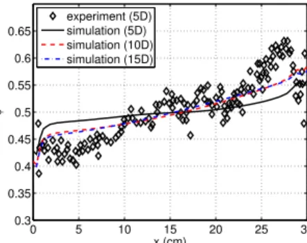
A first computation was carried out on a fixed mesh by considering that the pipe moved from right to the left and the pistons were maintained fixed. This way a reference solution was obtained using an Eulerian approach. The mesh for this simulation has 52,569 nodes and is formed by 257,280 tetrahedral elements. Particle segregation for different positions of the pis-ton is shown in Figure 9. The solid fraction decreases in front of the pispis-ton and is higher in the second half of the domain along the pipe axis. This is in agreement with experimental observation (Subia et al., 1998). The mean solid fraction on sections normal to the pipe axis was computed and plotted along the pipe axis in Figure 10. The results are compared with experimental data collected after the piston was displaced with 5 piston diameters. The nu-merical solution recovers correctly the segregation behaviour, but slightly underestimates the change in the solid fraction. However, the agreement with previously published numerical results (Fang et al., 2002) is very good. Simulation indicates that the segregation in front of a moving piston evolves quite rapidly and that an almost developed flow is attained after a 10D piston displacement.
(a) After 5D (b) After 10D
(c) After 15D
0 5 10 15 20 25 30 0.3 0.35 0.4 0.45 0.5 0.55 0.6 0.65 x (cm) φ experiment (5D) simulation (5D) simulation (10D) simulation (15D)
Figure 10. Mean solid fraction along the tube axis using an Eulerian approach (experimental data from (Subia et al., 1998))
This problem describes well the behaviour of the material in front of the plunger during in-jection moulding. However, simulation of the piston movement in material processing would not be possible in an Eulerian frame of reference, since the model includes both the moving piston and stationary parts as the mould cavity. Therefore the more general Arbitrary La-grangian Eulerian (ALE) formulation is used as described in (Ilinca & H´etu, 2008b). The ALE simulation was carried out on a mesh with 104,489 nodes and 499,200 tetrahedral elements. There were 16 elements in radial direction, 48 elements along the piston circumference and 160 elements along the pipe axis. Results using the ALE formulation for the piston driven flow with a free surface are shown in Figures 11 and 12. Figure 11 illustrates the solid fraction distribution in a cross-section along the pipe axis. It shows also the change in the computa-tional domain (gray rectangles) and the form of the free surface on the right hand end of the filled region. The results are very close to those given by the Eulerian approach (Figures 9 and 10). Small differences are observed at the right end of the computational domain, where a non-planar free surface is present in the ALE solution and a flat no-slip surface is present in the Eulerian case. The agreement between the two sets of computations indicates that the ALE approach performs well and can be used for injection moulding applications.
(a) Initial solution (b) After 5D
(c) After 10D (d) After 15D
Figure 11. Computational domain and distribution of solid fraction for various piston dis-placements (ALE formulation)
The particle migration towards the center of the flow through a tube and the buildup of higher solid particle concentration in the vicinity of the free surface is well
doc-0 5 10 15 20 25 30 0.3 0.35 0.4 0.45 0.5 0.55 0.6 0.65 x (cm) φ experiment (5D) simulation (5D) simulation (10D) simulation (15D)
Figure 12. Mean solid fraction along the tube axis using an ALE approach (experimental data from (Subia et al., 1998))
umented by experimental observation (Karnis & Mason, 1967; Seshadri & Sutera, 1967; Ramachandran & Leighton, 2007). Tang et al. (2000) associated the observed instability of the fluid/air interface interface under specific conditions to the particle accretion in the meniscus region. In the present piston driven flow the particle concentration is significantly higher in the right handside of the tube. To illustrate this phenomenon we divided the flow domain shown in Figure 8 into two equal size sub-domains: one for x<L/2 and the other for x>L/2
(x=L/2 denotes the middle of the fluid region). One can observe that the region near the center of the pipe has higher flow rate and also higher particle concentration. Thus, even if the net flow exchange between the left and right sub-domains is zero, there is a non-zero par-ticle flux across the surface between the two sub-domains at x=L/2 as shown in Figure 13(a). The mean volumetric particle concentration in the left and right sub-domains is shown in Fig-ure 13(b). A positive particle flux indicates that more particles are transported from the left towards the right sub-domain than in the opposite direction. Therefore the mean volumetric particle concentration increases in the right side. This hapens until t=1000s, from which point the left/right particle migration reverses and the net particle flux is from the right towards the left side. 0 200 400 600 800 1000 1200 −1 −0.5 0 0.5 1 1.5 2x 10 −3 time(s) (u ⋅ φ )m
Particle flow rate at x=L/2
(a) Net particle flux across x=L/2
0 200 400 600 800 1000 1200 0.4 0.45 0.5 0.55 time(s) φm
Volume average concentration (global) Volume average concentration (x<L/2) Volume average concentration (x>L/2)
(b) Mean volumetric particle concentration
4.5 Segregation during mould filling
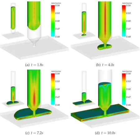
In this application the ALE formulation is used to predict powder segregation during the in-jection moulding of a rectangular plate (Ilinca & H´etu, 2008a). The plate is 8cm by 6cm and has 4mm in thickness. The filling piston has a radius of 1cm and his displacement is 13.2cm. Filling of the plate is made through a circular gate with a radius of 2mm. The suspension con-tains particles of 100µm in diameter and the initial solid fraction is uniform at 50%. Complete filling of the plate takes 10.0s. The filling pattern and the solid fraction distribution is shown in Figure 14 after 1.8s, 4.0s, 7.2s and respectively 10.0s.
(a) t=1.8s (b) t=4.0s
(c) t=7.2s (d) t=10.0s
Figure 14. Distribution of solid fraction for the injection of a plate.
The figure shows a cut along the symmetry plane parallel to the longest side of the plate in order to see the solid fraction distribution inside the part. The images show both the complete domain, where the displacement of the piston during the filling is clearly seen, and details of the flow inside the plate. Segregation of solid particles is apparent inside the pipe as pre-viously observed for the piston driven flow case. This causes the material to enter the gate with a non-uniform solid fraction. Additional segregation is observed inside the gate where shear rates are highest. The moulded part has higher solid fraction in the mid-plane and on the boundaries of the plate (far from the gate) and lower solid fraction on the upper and lower surfaces.
−1 −0.5 0 0.5 1 0.3 0.35 0.4 0.45 0.5 0.55 0.6 r/Rg φ Gate inlet Gate mid−length Gate end
(a) Concentration inside the gate
0 0.2 0.4 0.6 0.8 1 0.4 0.45 0.5 0.55 y/H φ z=1cm z=2cm z=3cm
(b) Concentration across the thickness of the plate
Figure 15. Distribution of solid fraction for the injection of a plate.
The particle concentration at the end of the filling time for various locations inside the gate and along the plate is shown in Figure 15. Figure 15(a) shows the solution at gate inlet and outlet, as well as midway between the two locations. The gate length is 5mm. Note that particle concentration increases near the gate axis, where velocities are higher. At the exit from the gate the particle concentration decreases significantly near the walls. Particle distribution across the thickness of the plate at 1, 2, and respectively 3cm from the gate (in the center plane parallel to the longest side) are shown in Figure 15(b). In all sections the concentration is higher in the center and lower at the walls.
5. Conclusion
A three-dimensional finite element algorithm for the solution of injection moulding is pre-sented. Numerical solutions are validated against experimental data for the filling-packing of a rectangular plate and then the methodology is applied to co-injection, gas-assisted injection and powder injection moulding. The algorithm is very robust and provide accurate solutions. It is able to recover three-dimensional phenomena as the thickness distribution of skin and core polymers in co-injection and the gas penetration for gas-assisted injection. For powder injection moulding the segregation of solid particles is solved using a diffusive flux model. For the piston driven flow the ALE formulation is shown to provide similar results as an Eulerian approach on a fixed mesh, thus indicating that the procedure performs well. Application to the mould filling of a rectangular plate shows the ability to use this method to the solution of powder injection moulding.
6. References
Baaijens, F.P.T. & Douven, L.F.A. (1991). Calculation of flow-induced residual stresses in injec-tion moulded products. Applied Scientific Research, Vol. 48, pp. 141-157.
Chen. B.S. & Liu, W.H. (1994). Numerical simulation of the post-filling stage in injection mold-ing with a two-phase model, Polymer Engineermold-ing and Science, Vol. 34, pp. 835–847.
Chen, S.C. & Hsu, K.F. (1995). Numerical Simulation and Experimental Verification of Melt Front Advancements in Coinjection Molding Process. Numerical Heat Transfer, Part A, Vol. 28, p.503.
Chen, S.C.; Cheng, N.T. & Hsu, K.S. (1995). Simulations of gas penetration in thin plates de-signed with a semicircular gas channel during gas-assisted injection moulding, Int. J. Mech. Sci.. Vol. 38, pp. 335–348.
Chiang, H.H.; Hieber, C.A. & Wang, K.K. (1991). A unified simulation of the filling and post-filling stages in injection molding. Part I: Formulation. Polymer Engineering and Sci-ence, Vol. 31, pp. 116–124.
Chiang, H.H.; Hieber, C.A. & Wang, K.K. (1991). A unified simulation of the filling and post-filling stages in injection molding. Part II: Experimental verification. Polymer Engi-neering and Science, Vol. 31, pp. 125–139.
Fang, Z.; Mammoli, A.A.; Brady, J.F.; Ingber, M.S.; Mondy, L.A. & Graham, A.L. (2002). Flow-aligned tensor models for suspension flows, Int. J. of Multiphase Flow, Vol. 28, pp. 137– 166.
Franca, L.P. & Dutra do Carmo, E.G. (1989). The Galerkin Gradient Least-Squares Method. Computer Methods in Applied Mechanics and Engineering, Vol. 74, p.41.
Franca, L.P. & Frey, S.L. (1992) Stabilized finite element methods: II. The incompressible Navier-Stokes equations. Computer Methods in Applied Mechanics and Engineering, Vol. 99, p.209.
Gao, D.; Nguyen, K.; Garcia-Rejon, A.; Salloum, G. (1997). Numerical modelling of the mould filling stage in gas-assisted injection moulding, Int. Polym. Proc., Vol. 12, pp. 267–277. Han, K.-H. & Im, Y.-T. (1997). Compressible flow analysis of filling and post-filling in injection
molding with phase-change effect, Composite Structures, Vol. 38, pp. 179–190. H´etu, J.-F., Gao, D.M., Garcia-Rejon, A. & Salloum, G. (1998). 3D finite element method for the
simulation of the filling stage in injection molding. Polymer Engineering and Science, Vol. 38, pp. 223–236.
Hieber, C.A. & Shen, S.F. (1980). A finite-element/finite-difference simulation of the injection-molding filling process. J. Non-Newtonian Fluid Mechanics, Vol. 7, pp. 1–32.
Ilinca, F., H´etu, J.-F. & Pelletier, D. (2000). On Stabilized Finite Element Formulations for Incompressible Advective-Diffusive Transport and Fluid Flow Problems. Computer Methods in Applied Mechanics and Engineering, Vol. 188, pp. 235–255.
Ilinca, F. & H´etu, J.F. (2001). Three-dimensional filling and post-filling simulation of polymer injection molding. International Polymer Processing, Vol. 16, p.291.
Ilinca, F. & H´etu, J.-F. (2002). Three-Dimensional Finite Element Solution of Gas-Assisted In-jection Moulding, Int. J. Num. Methods Engng., Vol. 53, pp. 2003–2017.
Ilinca, F., H´etu, J.-F., Derdouri, A. & Stevenson, J. (2002). Metal Injection Molding: 3D Model-ing of Nonisothermal FilModel-ing. Polymer EngineerModel-ing and Science, Vol. 42, pp. 760–770. Ilinca, F. & H´etu, J.F. (2002). Three-dimensional numerical modeling of co-injection molding.
International Polymer Processing, Vol. 17, pp. 265–270.
Ilinca, F. & H´etu, J.-F. (2003). Three-dimensional simulation of multi-material injection mold-ing: Application to gas-assisted and co-injection molding. Polymer Engineering and Science, Vol. 43, pp. 1415–1427.
Ilinca, F.; H´etu, J.-F. & Derdouri, A. (2006). Numerical investigation of the flow front behaviour in the co-injection moulding process. International Journal for Numerical Methods in Fluids, Vol. 50, pp. 1445–1460.
Ilinca, F. & H´etu, J.F. (2008). Three-dimensional numerical simulation of segregation in powder injection molding. International Polymer Processing, Vol. 23, pp. 208–215.
Ilinca, F. & H´etu, J.-F. (2008). Three-dimensional free surface flow simulation of segregat-ing dense suspensions. International Journal for Numerical Methods in Fluids, Vol. 58, pp. 451–472.
Janeschitz-Kriegl, H. (1983). Polymer melt rheology and flow birefrengence, Springer-Verlag, pp. 424–448.
Kamal, M.R., Kuo, Y. & Doan, P.H. (1975). The injection molding behavior of thermoplastics in thin rectangular cavities. Polymer Engineering and Science, Vol. 15, pp. 863–868. Karnis, A. & and Mason, S.G. (1967). The flow of suspensions through tubes: VI.Meniscus
Effects, J. Colloid and Interface Sc., Vol. 23, pp. 120–133.
Kim, S.-W. & Turng. L.-S. (2004). Developments of three-dimensional computer-aided engi-neering simulation for injection moulding. Modeling and Simulation in Materials Sci-ence and Engineering, Vol. 12, pp. 151–173.
Phillips, R.J., Armstrong, R.C., Brown, R.A., Graham, A.L. & Abott, J.R., (1992). A constitu-tive equation for concentrated suspensions that accounts for shear-induced particle migration, Physics of Fluids, A, Vol. 4, pp. 30–40.
Polynkin, A., Pittman, J.F.T. & Sienz, J. (2005). Gas assisted injection molding of a handle: Three-dimensional simulation and experimental verification. Polymer Engineering and Science, Vol. 45, pp. 1049–1058.
Ramachandran, A. & Leighton Jr., D.T. (2007). The effect of gravity on the meniscus accumu-lation phenomenon in a tube, J. Rheol., Vol. 51, pp. 1073–1098.
Schlatter, G.; Davidoff, A.; Agassant, J.F. & Vincent, M. (1999). An Unsteady Multifluid Model: Application to Sandwich Injection Molding Process. Polymer Engineering and Science, Vol. 39, p.78.
Seshadri, V. & Sutera, S.P. (1967). Concentration changes of suspensions of rigid spheres flow-ing through tubes, J. Colloid and Interface Sc., Vol. 27, pp. 101–110.
Subia, S.R.; Ingber, M.S.; Mondy, L.A.; Altobelli, S.A. & Graham, A.L. (1998). Modelling of concentrated suspensions using a continuum constitutive equations, Journal of Fluid Mechanics, Vol. 373, pp. 193–219.
Tang, H.; Grivas, W.; Homentcovschi, D.; Geer, J. & Singler, T. (2000). Stability considerations associated with the meniscoid particle band at advancing interfaces in Hele-Shaw suspension flows, Physical Review Letters, Vol. 85, pp. 2112–2115.
Wimberger-Friedl, R. & Janeschitz-Kriegl, H. (1988). Residual birefringence in injection molded compact discs. First international conference on electrical, optical and acoustic properties of polymers, 22/1–22/10, Canterbury, UK, 1988.
Wu, S. (1991). Surface and interfacial tensions of polymers, oligomers, plasticizers and organic pigments. Polymer Handbook, Ed. J.Brandup, EH Immergut EA Grulke, pp. 521–541.