Graphical user interface development for ocean models

(1)

Publisher’s version / Version de l'éditeur:

Vous avez des questions? Nous pouvons vous aider. Pour communiquer directement avec un auteur, consultez la

première page de la revue dans laquelle son article a été publié afin de trouver ses coordonnées. Si vous n’arrivez pas à les repérer, communiquez avec nous à PublicationsArchive-ArchivesPublications@nrc-cnrc.gc.ca.

Questions? Contact the NRC Publications Archive team at

PublicationsArchive-ArchivesPublications@nrc-cnrc.gc.ca. If you wish to email the authors directly, please see the first page of the publication for their contact information.

https://publications-cnrc.canada.ca/fra/droits

L’accès à ce site Web et l’utilisation de son contenu sont assujettis aux conditions présentées dans le site LISEZ CES CONDITIONS ATTENTIVEMENT AVANT D’UTILISER CE SITE WEB.

Student Report (National Research Council of Canada. Institute for Ocean Technology); no. SR-2006-04, 2006

READ THESE TERMS AND CONDITIONS CAREFULLY BEFORE USING THIS WEBSITE.

https://nrc-publications.canada.ca/eng/copyright

NRC Publications Archive Record / Notice des Archives des publications du CNRC :

https://nrc-publications.canada.ca/eng/view/object/?id=36e360a7-9946-49d8-961c-d4ae7eb34066 https://publications-cnrc.canada.ca/fra/voir/objet/?id=36e360a7-9946-49d8-961c-d4ae7eb34066

NRC Publications Archive

Archives des publications du CNRC

For the publisher’s version, please access the DOI link below./ Pour consulter la version de l’éditeur, utilisez le lien DOI ci-dessous.

https://doi.org/10.4224/8895453

Access and use of this website and the material on it are subject to the Terms and Conditions set forth at

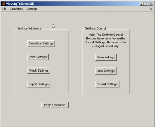
Graphical user interface development for ocean models

Noel, A.

(2)

DOCUMENTATION PAGE

REPORT NUMBER

SR-2006-04

NRC REPORT NUMBER DATE

April 19, 2006

REPORT SECURITY CLASSIFICATION

Unclassified

DISTRIBUTION

Unlimited

TITLE

GRAPHICAL USER INTERFACE DEVELOPMENT FOR OCEAN MODELS

AUTHOR(S)

Adam J. G. Noel

CORPORATE AUTHOR(S)/PERFORMING AGENCY(S)

PUBLICATION

Institute for Ocean Technology

SPONSORING AGENCY(S)

Institute for Ocean Technology

IOT PROJECT NUMBER

PJ2019

NRC FILE NUMBER KEY WORDS

Graphical user interface, industry company profile, software, manoeuvring PAGES 17 + app. FIGS. 0 TABLES 0 SUMMARY

An overview of the field of ocean research is presented, including a summary of organizations that are active in the Canadian Atlantic region. The National Research Council’s Institute for Ocean Technology (NRC-IOT) is described with respect to its capabilities to conduct research and its primary focus areas. Finally, the role of the author throughout the Winter 2006 work term is discussed, outlining the development of a graphical user interface (GUI) for ocean software models.

ADDRESS National Research Council

Institute for Ocean Technology Arctic Avenue, P. O. Box 12093 St. John's, NL A1B 3T5

(3)

National Research Council Conseil national de recherches Canada Canada

Institute for Ocean Institut des technologies Technology océaniques

GRAPHICAL USER INTERFACE DEVELOPMENT FOR OCEAN MODELS

SR-2006-04

Adam J. G. Noel

(4)

i

ACKNOWLEDGEMENTS

Gavin Earle, Ping Xiao, Jiancheng Liu, and Dr. Wayne Raman-Nair provided in-house software models. Their assistance in integrating their work with the author’s is greatly appreciated.

Wayne Pearson, Greg Janes, Jim Millan, and Bruce Quinton provided advice on various aspects of the Matlab environment, and a thank-you goes to them as well.

Finally, the author also thanks Dr. Michael Lau for continuous support and mentoring throughout the Winter 2006 work term.

(5)

ii

ABSTRACT

An overview of the field of ocean research is presented, including a summary of

organizations that are active in the Canadian Atlantic region. The National Research Council’s Institute for Ocean Technology (NRC-IOT) is described with respect to its capabilities to conduct research and its primary focus areas. Finally, the role of the author throughout the Winter 2006 work term is discussed, outlining the development of a graphical user interface (GUI) for ocean software models.

(6)

iii TABLE OF CONTENTS Acknowledgements... i Abstract ...ii Appendices...iii 1.0 Introduction... 1

2.0 Profile of Ocean Research ... 2

2.1 Origins and History... 2

2.2 Presence of the Field Today... 3

2.3 Continuing Evolution... 5 3.0 IOT Profile ... 6 3.1 Background ... 6 3.2 Facilities ... 6 3.3 Organizational Structure ... 7 3.4 Client Base ... 8 3.5 Future Development... 9 4.0 Student’s Role... 11 4.1 Primary Roles... 11 4.2 Other Duties ... 12

4.3 The Work Environment ... 12

4.4 Job Challenge and Educational Enhancement ... 13

4.5 GUI Development ... 14

4.5.1 Moving Triangle Demonstration... 14

4.5.2 Moving Triangle Demonstration in Three Dimensions ... 15

4.5.3 Ocean-Structure Interactions Simulator... 15

5.0 References... 17

APPENDICES

Appendix A: GUI Figures

(7)

Graphical User Interface Development for Ocean Models

1

1.0 INTRODUCTION

This report is the author’s industry company profile (ICP), completed as required for Memorial University of Newfoundland’s Faculty of Engineering and Applied Science. The ICP is a requirement for work term 2 and will be graded by Co-operative Education. Secondly, this report satisfies the requirement of a technical report for the National Research Council of Canada’s Institute for Ocean Technology (NRC-IOT), where the author completed the Winter 2006 work term.

An overview of the field of ocean research is presented, including a summary of

organizations that are active in the Canadian Atlantic region. IOT is described with respect to its capabilities to conduct research and its primary focus areas. Finally, the role of the author for the work term is discussed. This component outlines the development of a graphical user interface (GUI) for ocean software models.

A number of other reports were completed in conjunction with this report that focus on the creation and use of the GUIs. The “User’s Manual for MTD3D” (Noel, 2006) and “User’s Manual for OSIS (Ocean-Structure Interactions Simulator) v0.5 – Version 1” (Noel and Lau, 2006) are general use references for two versions of the GUI. The development and

programming details of OSIS is discussed in much greater detail in “GUI Programmer Manual for OSIS (Ocean-Structure Interactions Simulator) – Version 1” (Noel and Lau, 2006). Please refer to these documents for additional information.

(8)

2

2.0 PROFILE OF OCEAN RESEARCH

2.1 Origins and History

Human beings have been using the oceans of the world for different purposes for thousands of years. Sailing vessels throughout history were designed for transportation, warfare, and the gathering of resources.

Primitive humans began ocean travel by vessel, likely using simple rafts. By 6000 BC, hallowed logs were being used for fishing off the coasts of northern Europe. War craft have existed on the Nile since 9000 BC (Woodman, 1997). From these early times, vessels have undergone significant evolutions.

The fishery was the predominant resource for many centuries, however the use of natural gases for transportation and heating, combined with rising oil prices, has led to the importance of the offshore oil and gas sector. Onshore oil wells have been present in North America since the nineteenth century (McKenzie-Brown et al., 1993), however it was not until 1947 that offshore production began by American companies in the Gulf of Mexico (Pratt et al., 1997). The rising cost of oil has steadily driven the industry out to deeper and harsher waters in environments that are more hostile, such as those in northern climates.

Much of the field of ocean research today is thus somehow related to the offshore oil and gas industry, which has a very strong presence in the Atlantic region. Offshore wells have been drilled in this region for over forty years, however it is only within the last fifteen years that the commercial extraction of crude oil has begun in Atlantic Canada (Locke, 1999). Ocean research has investigated many aspects of this process, including the dynamics and design of oil

(9)

3

2.2 Presence of the Field Today

A number of organizations today are involved with ocean research. Due to geographical considerations, there is a strong presence in the Canadian Atlantic region, particularly in Newfoundland. A significant proportion of the research and development performed is in relation to operations in harsh environments, such as extreme climates, deep waters, and the presence of ice. Studies continue to be made, not only in relation to offshore oil and gas, but also with general cargo transport, fishing and aquaculture, competitive racing, and surveillance.

The Newfoundland Ocean Industries Association (NOIA) was formed in 1977, with a broad mandate to be a collective body of companies with interests in ocean industries. Today the NOIA has about five hundred member companies in Eastern Canada, focussed on the oil and gas

industry. The Association members have been involved with all facets of the industry, including development, production, construction, transport, processing, and research and development. The NOIA itself is a non-profit organization providing lobbying and networking opportunities to the industry (Newfoundland Ocean Industries Association, 2006).

Petroleum Research Atlantic Canada (PRAC) aims to foster research and development in the petroleum industry by supporting inter-disciplinary work. Beginning operations in 2002, the PRAC is a public-private partnership providing funding via grants and contract research.

Completed projects cover the entire spectrum of fields in the industry, from numerical modelling and safety tests to geological studies and socio-economic benefits (Petroleum Research Atlantic Canada, 2006). Its members include oil and gas corporations such as Petro-Canada and

ExxonMobil, provincial and federal government departments, and Atlantic Canada academic institutions such as Memorial University of Newfoundland (MUN) and Dalhousie University. It should be noted that PRAC is a member body of the NOIA.

(10)

4

A local corporation based in St. John’s that is a key partner in ocean research is C-CORE. Formed in 1975, C-CORE has facilities on the MUN campus and they have a long history of working with the offshore oil and gas industry. As a corporation, their work is conducted via funded projects and contracts for research and development and the applications of new

technologies. C-CORE has expanded its interests to include other fields such as mining and pulp and paper. While initially working almost exclusively with large corporations, downsizes in the 1980s prompted a shift to partnering with small and medium size enterprises, a trend that continues to this day (C-CORE, 2006). C-CORE is also a member body of the NOIA.

It would be more than reasonable to assume that any industry involving research will have extensive connections to the academic world. While the aforementioned organizations have strong ties to academia, there are others that are even more integrated with post-secondary institutions. The Centre for Marine Simulation (CMS) is an operational unit of the School of Maritime Studies at the Marine Institute. Its advanced technology was created for the training of navigators and other mariners for harsh environment, yet has evolved to play a role in

prototyping, development of work procedures, and testing of new equipment. For example, CMS has been used for simulating the towing of the Hibernia gravity-based structure and for Coast Guard training programs (Centre for Marine Simulation, 2006). Secondly, the Ocean

Engineering Research Centre (OERC) is an integrated part of MUN’s Faculty of Engineering and Applied Science Ocean and Naval Architectural program. The OERC has its own towing tank for conducting research efforts, and its facilities are available to students as well as faculty and contract clients (Faculty of Engineering and Applied Science, 2006).

Other corporations have fewer ties to the academic world. One such corporation is

(11)

5

the province’s primary flight carrier to conducting surveillance of Canada’s oceans for the federal government. Extensive research is undertaken for the development of their surveillance craft for the east and west offshore regions of the country (Scott, 2006). Another corporation, Marport Ltd., is creating sophisticated sensors for trawlers and attempting to introduce wireless broadband for offshore environments (Riggs, 2006). These companies are connected via

OceansAdvance, an ocean technology cluster development forum. OceansAdvance seeks ocean-related industry growth as a whole by improving communications between different companies, academic institutes, and government (O’Reilly, 2006).

2.3 Continuing Evolution

It suffices to say that the field of ocean research in the Atlantic region is one that is

continuously evolving. The development of new technologies is creating many opportunities for the field. As a whole, the ocean/marine technology sector is the fastest growing in the province, with growth of 15-20% annually from 1998 to 2003 (O’Reilly, 2006).

As the technologies driving marine simulations and design advance, the importance of teamwork grows. The field will expand with collaborations of groups and individuals of different technical backgrounds. Organizations such as the NOIA and OceansAdvance will foster

partnerships so that projects can be completed in as effective a manner as possible. Within

companies, it will become more important to have individuals from various fields of engineering, arts, economics, and the sciences.

The prominence of the offshore oil and gas industry is expected to continue for at least the next twenty years; society’s need for these resources will fuel research projects in this area. This includes the development of oil and gas projects in northern environments.

(12)

6

3.0 IOT PROFILE

3.1 Background

The Institute for Marine Dynamics (IMD) was opened in 1985 by the National Research Council of Canada (NRC). The Institute was created with the goal of supporting ocean

technology industries across the country by combining experience with extensive facilities. As a government facility, the Institute has provided a broad range of services and products to public, private, and sporting ocean industries. The Institute was renamed the Institute for Ocean

Technology (IOT) in 2004 to better reflect its achievements and goals.

3.2 Facilities

The facilities located and maintained at IOT are among the most extensive in the world for ocean research. Each component offers unique services and opportunities.

The three major facilities are the Offshore Engineering Basin, the Towing Tank, and the Ice Tank. The Basin can produce waves, current, and wind, re-creating the harsh ocean environment for testing oil platforms and other models. Ship models can be up to 4.5 metres in length, while platform structures can be up to 6 metres in diameter. The Towing Tank is 200 metres in length and has its own wave-maker. It can support ship models up to 12 metres in length or platforms up to 4 metres in diameter. The Ice Tank, 90 metres in length, can use ice sheets of length up to 76 m, the longest in the world, while also doubling as a second tow tank.

Many other resources complement the major facilities. There is a cavitation tunnel for performing tests on propellers and conducting other force and pressure tests. Two cold rooms, one large and one small, can obtain temperatures as low as –40 degrees Celsius and create ice for the ice tank while being able to perform their own tests for crystal structure and other model ice

(13)

7

properties. Various pieces of equipment are available for test measurements, from capacitance probes for waves and dynamometers for propeller shafts, to more advanced mechanisms. The Yacht Dynamometer was designed specifically for measuring lift and drag on models for the America’s Cup competition. The Marine Dynamic Test Facility can monitor underwater vehicles moving with six degrees of freedom. The Planar Motion Mechanism (PMM) is used for

manoeuvrability studies, particularly those of models in ice conditions.

IOT also has the capability of fabricating the models used at its facilities, with specialized equipment for working with small-scale construction. The computerized five-axis milling machine can make wooden and high density foam models up to 12 metres in length.

3.3 Organizational Structure

As noted, IOT is one of the Institutes of the National Research Council of Canada (NRC). NRC is a federal government agency, so IOT receives its funding directly from the federal government.

The head of the Institute is the Director General, a position currently held by Dr. Mary Williams. The rest of the Institute is divided into seven major categories: research, facilities, quality and planning, human resources, communications, finance, and business development, each with their own respective director. The majority of the employees work in the research and facilities divisions, since the focus of IOT is as a research facility. The facilities division can be further divided into the ice tank, electronics, computer systems, software engineering, open water test facilities, design and fabrication, and engineering support and maintenance.

Much of the research conducted is project based, with each project having a supervisor and other members. Members can be directly involved with multiple projects at once, depending on the time required and the individual expertise they bring. Projects may or may not be directly

(14)

8

applicable to industry, however most can be placed into one of the five focus research areas that IOT has identified.

The first research area is that of ships and structures in ice, with the goal to predict ship and structure performance in ice conditions using a combination of numerical and physical models. A more general area is that of performance evaluation in the ocean environment, which investigates performance at sea but not necessarily in ice. The area of underwater vehicle systems is

developing the means for exploration and manipulation of sub-sea environments. This area is similar to that of applied hydrodynamics, which predicts structure dynamics for sub-sea resource discovery. The marine safety area tests lifesaving systems and safe operation of smaller vessels. All of these focus areas cover the broad scope of supporting ocean technology industries. Additionally, unique ideas can be allocated short-term efforts to determine the feasibility of further study.

3.4 Client Base

As a research facility, IOT maintains a unique client base with connections to both academia and industry. It has formed partnerships with a number of organizations, both directly and

indirectly.

The facilities over the years have been used for testing models of various ferries, oil platforms, ice-breakers, racing yachts, life craft, ships, and submersibles. Clients for these tests include crown corporations such as Marine Atlantic, large partnerships such as the Hibernia development project, and competitors in the America’s Cup races. These services have generally been arranged via contract. The internal project groups for research, who can in turn offer their results to companies in the industry at large and have their work presented to the academic community, use a significant portion of the facilities.

(15)

9

Currently, most of the external contracting is conducted via Oceanic, which was created as a collaboration of IOT and Memorial University of Newfoundland. Formed in 1998, Oceanic offers commercial and public enterprises access to all of IOT’s testing facilities, and their clients have included designers of commercial ships, fixed and floating offshore platforms, government ships, passenger vessels, and sub-sea systems.

IOT helps start-up companies with their ventures via OTEC, the Ocean Technology Enterprise Centre. Various programs within OTEC, such as the Young Entrepreneurs Program and the Ocean Technology Co-Location Program, offer funding and/or facilities to new

companies in the field. Current co-locating companies include Madrock Marine Solutions, a developer of marine safety products, LewHill Testing Technologies, a developer of temperature and pressure calibration systems, NavSim Technologies, a designer of electronic navigation systems, and Shearwater Geophysical, who conduct seismic consulting. Current participants in the Young Entrepreneurs Program include Virtual Marine Technology and WES Power

Technologies.

3.5 Future Development

IOT will continue to perform as a local, national, and worldwide leader in ocean technology research. It will adapt to the evolution of industry needs as required, and foster the formation of other organizations within the St. John’s ocean engineering technology cluster.

Since most of the facilities within the Institute are now over twenty years old, a significant effort is in place for infrastructure replacement. High maintenance costs, decreased reliability, and the use of many components beyond their expected operational life are driving the need to replace equipment. A five-year plan formed in 2004 has been dedicating hundreds of thousands

(16)

10

of dollars annually to this effort. The infrastructure replacement is expected to assist in the Institute’s goal to offer state-of-the-art facilities.

IOT will remain supportive of OTEC, which will continue to promote growth and development of companies in the field. This will be key in ensuring that the field of ocean research will maintain growth in the province. As noted, ocean technology is the fastest growing sector in Newfoundland and Labrador, so it is expected that there will be a growing market to benefit from ocean research.

(17)

11

4.0 STUDENT’S ROLE 4.1 Primary Roles

One of IOT’s primary research areas is that of ships and structures in ice conditions, with the goal to make predictions from models to determine the reaction and performance of ships and structures in ice. Software development project PJ2019 is part of this research initiative and includes the development of a model for a moored cone in ice, eventually expanding to other model cases. The software model requires an effective graphical user interface (GUI), whose design and implementation was the primary focus of this author’s experience.

The GUI faced a number of requirements for its design. It was necessary to create an interface that would be accessible to users who would not be expected to fully understand the models upon which the software was based. The interface needed to be sufficient for use without having to enter or modify any programming code, contrary to many models currently available. The interface itself could not be limited to a single model, but rather act as a platform for different models that could be integrated as the software evolved. Finally, there had to be sufficient documentation included so that other programmers could easily pick up and expand the code.

For the duration of the work term, it was expected that the GUI would be developed and made available as proof of concept to showcase the capabilities that an intuitive and integrated interface could have when applied to pre-existing and newly developed models. An attempt would be made to implement a variety of ideas. Matlab was chosen as the development language because of its GUI-creating tools, its high-level language format, and its presence as a language for model design.

(18)

12

In addition, time was also dedicated for the editing of various research reports that were in different stages of development, from initial drafts to final compiled copies. The format to be followed was that specified in the “IOT Publications Manual” (LeBlanc et al., 2004), which provided guidelines for font, heading styles, figures, references, and appendices. Many of the reports required re-formatting to adhere to the guidelines.

4.2 Other Duties

A number of other tasks and activities were completed by the author. Meeting times and locations were arranged and booked, and minutes were created and sent to attendees for all project group meetings. A research video collection was in the process of being upgraded to DVD; the video inventory was updated, re-organized, and the videos were placed into the order specified by the inventory. The collection was comprised mostly of model tests, including those captured during the tests of the Kulluk scale model as part of PJ2019, as well as other tests throughout the last twenty years. About two hundred discs made up the inventory.

4.3 The Work Environment

The author’s work term was conducted at the National Research Council’s Institute for Ocean Technology in an office environment. The GUI design and implementation was performed independently, however there was considerable interaction with other individuals, including all of those involved with the software development project PJ2019. The project supervisor, Dr. Michael Lau, was in continued contact throughout the semester via email and regular meetings. The other project members, Gavin Earle and Ping Xiao, were also in regular contact. They were involved with providing feedback on aspects of the GUI, especially regarding models they had developed or modified for integration.

(19)

13

The GUI was created completely in Matlab Version 7 (Release 14, Service Pack 2), in part using its GUI Development Environment (GUIDE). An Intel Pentium 4, Hyper-Threading 3.0 GHz processor was used with 512 MB of RAM and running Windows XP Professional.

4.4 Job Challenge and Educational Enhancement

The work conducted required numerous skills to be completed in an effective manner, the most apparent being able to learn independently as necessary. The author had no previous experience with Matlab, however he had created a preliminary GUI within two weeks of

exposure. Working in Matlab was a continuous process of learning, especially when adding new features to the platform and de-bugging the code, while also providing an outlet for creativity when designing the interface and organizing the platform. A portion of related coding was performed in Fortran, with which the author also had no previous experience. Having completed two courses in programming with C++ was certainly beneficial to learning Matlab and Fortran, but it was also necessary to reference official documentation, educational texts, and online help services. It was also useful to speak with other individuals at the institute who worked with the Matlab and Fortran environments. The ability to independently learn computing languages will be an invaluable asset, not only from a programming perspective but also for learning in general.

The report editing required strong grammatical knowledge, an eye for identifying

discrepancies, and a desire to ensure that a given paper was as consistent as possible. The author gained exposure to technical writing in a research format while also learning about the field of structure-in-ice interactions. These abilities extended to the compiling of the reports for the GUI platform, including the user manuals and programming documentation, in addition to the

(20)

14

It is expected that the work term will have a substantial influence on the author’s long-term goals. The team-focussed project environment will lend itself to any other professional

experiences, particularly those requiring communication and organizational abilities. The programming aspect will be beneficial to any future need to acquire more programming skills. Finally, the documentation experience will go a long way to develop the writing abilities needed as a professional engineer, academically or otherwise.

4.5 GUI Development

The process of GUI creation for PJ 2019 and related projects was, as noted, the primary focus of the author’s work. This process included interface design, implementation of exporting capabilities, and integration with pre-existing models. The GUI evolved a number of times to adapt to the requirements. Refer to Appendix A: GUI Figures for a series of figures highlighting the changes made to the GUI. All of the details of the development history are provided in “GUI Programmer Manual for OSIS (Ocean-Structure Interactions Simulator) – Version 1” (Noel and Lau, 2006).

4.5.1 Moving Triangle Demonstration

The first iteration of the GUI was to create a simple interface for a user to specify simulation parameters, view the results as they were generated, and conduct analysis with the results. The program was named Moving Triangle Demonstration, and was created within a few weeks of being introduced to Matlab. The simulation plotted a triangle moving on a

two-dimensional plot. The plot could be exported as a figure file, and its data could be exported to a simple Excel spreadsheet or text file. A previous progress report on this iteration is described in Appendix C of “User’s Manual for MTD3D” (Noel and Lau, 2006).

(21)

15

4.5.2 Moving Triangle Demonstration in Three Dimensions

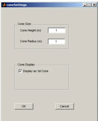
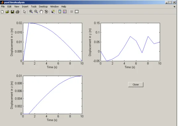
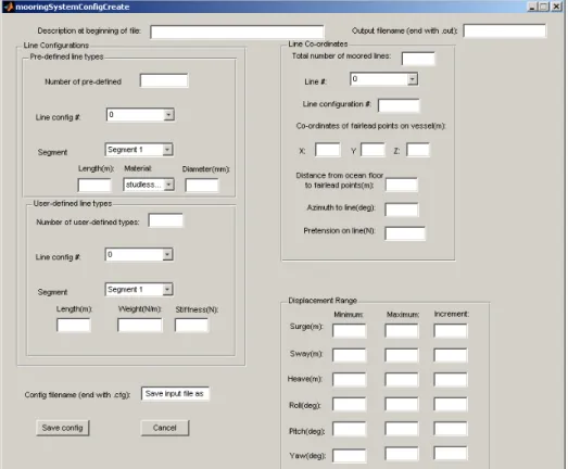
The next logical step was to expand the simulation to the third dimension and modify the interface to display it. Aptly named Moving Triangle Demonstration in Three Dimensions (MTD3D), the program plotted a cone object moving on a three-dimensional plot.

Gradually, over the period of a month and a half, many other features were introduced to MTD3D. AVI video generation, settings files, and customized figure editing were among the capabilities introduced. The controls for the settings became organized into different windows based on category. Readouts displayed the current co-ordinates of the cone while its position was re-calculated. The simulation performing the calculations changed from arbitrary trigonometric formulas to a preliminary Simulink model designed by Gavin Earle. A separate interface from within MTD3D was created to write the input file required by the “mooring_system” Fortran program. The user manual for MTD3D is “User’s Manual for MTD3D” (Noel and Lau, 2006).

4.5.3 Ocean-Structure Interactions Simulator

MTD3D was found to have inherent limitations that prevented it from fulfilling the GUI requirements, although it was very useful for internally showcasing what an interface could do. There was no way to easily implement multiple models, i.e. create a platform, without re-designing the program. The nature of models to be included did not lend well to displaying results as they were calculated; the Simulink model, for example, needed to run in full before results became available.

The GUI was re-built to address these needs, in some cases recycling much of the code. It was named the Ocean-Structure Interactions Simulator (OSIS) to be more inclusive of its

capabilities. Its implementation occupied much of the final month and a half of the author’s term. OSIS separates simulations from analysis and uses custom text files for settings, simulation

(22)

16

output, and video configurations. The text files are created such that they can be read and understood if opened external of Matlab. A user can specify the model to be used in a specific simulation so that a relevant configuration window appears. The analysis allows plotting of any output data created by the simulation. AVI videos can be previewed and created to plot a specified object with given settings.

OSIS has already been used as a platform for ocean software models. Donald E. Nevel’s Fortran “Cone” (Nevel, 1992) program was compiled by the author for use with Matlab and then completely integrated with OSIS. Dr. Wayne Raman-Nair’s model for a steel riser in water (Raman-Nair and Baddour, 2005), created in Matlab, has had parameters accessible to the OSIS interface for input and output analysis. As part of PJ 2019 and PJ 2114, a combination of models created by Ping Xiao and Jiancheng Liu to calculate time-domain forces and displacements were introduced to OSIS for manipulation.

All of the code components of OSIS have been extensively documented in “GUI

Programmer Manual for OSIS (Ocean-Structure Interactions Simulator) – Version 1” (Noel and Lau, 2006). This report also includes development history and the process of adding new models and object types. General use of OSIS is described in “User’s Manual for OSIS (Ocean-Structure Interactions Simulator) v0.5 – Version 1” (Noel and Lau, 2006).

OSIS will be expanded even more as PJ 2019 continues. It already includes a significant number of features without a user needing to modify any code by providing continuous

interaction with an interface. Appendix B: Matlab Programming and GUI Fundamentals was created as a reference for any programmer new to Matlab or GUI design, and should be a helpful supplement to the official Matlab documentation.

(23)

17

5.0 REFERENCES

C-CORE, 2006. “C-Core’s History.” Accessed 30 Mar. 2006. URL: http://www.c-core.ca/about/history.php

Centre for Marine Simulation, 2006. “About Us: Capability Statement.” Accessed Mar. 31, 2006. URL: http://www.mi.mun.ca/cms/cms_capability_statement.htm

Faculty of Engineering and Applied Science, 2006. “Ocean Engineering Research Centre (OERC).” Memorial University of Newfoundland. Accessed 31 Mar. 2006. URL: http://www.engr.mun.ca/research/centres/OERC/

LeBlanc, T., Green, E., and R.E. Baddour, 2004. “IOT Publications Procedures Manual.” NRC/IOT Report LM-2004-32, Institute for Ocean Technology, National Research Council of Canada, St. John’s, NL.

Locke, W., and Community Resource Services, 1999. Harnessing the Potential – Atlantic Canada’s Oil and Gas Industry. Strategic Concepts, Inc.

Mckenzie-Brown, P., Jaremko, G., and D. Finch, 1993. The Great Oil Age: The Petroleum Industry in Canada. Calgary: Detselig Enterprises Ltd., pp. 14-15.

Nevel, D.E., 1992. “Ice forces on cones from floes”, Proceedings of IAHR ’92, 11th International Symposium on Ice Problems, Banff, Alta., Vol. 3, pp. 1391–1404.

Newfoundland Ocean Industries Association, 2006. “About NOIA.” Accessed 10 Apr. 2006. URL: http://www.noianet.com/about/

Noel, A., and Lau, M., 2006. “GUI Programmer Manual for OSIS (Ocean-Structure Interactions Simulator) – Version 1”, NRC/IOT Report LM-2006-02 (Protected), Institute for Ocean Technology, National Research Council of Canada, St. John’s, NL.

Noel, A., and Lau, M., 2006. “User’s Manual for MTD3D”, NRC/IOT Report SR-2006-09, Institute for Ocean Technology, National Research Council of Canada, St. John’s, NL. Noel, A., and Lau, M., 2006. “User’s Manual for OSIS (Ocean-Structure Interactions Simulator)

v0.5 – Version 1”, NRC/IOT Report LM-2006-01 (Protected), Institute for Ocean Technology, National Research Council of Canada, St. John’s, NL.

O’Reilly, L., 2006. “OceansAdvance Forum – An Opportunity to Exchange Ideas.” Institute for Ocean Technology. St. John’s, NL, 6 Apr. 2006.

Petroleum Research Atlantic Canada, 2006. “What is PRAC?” Accessed 30 Mar. 2006. URL: http://www.pr-ac.ca/prac_4245.html

(24)

18

Pratt, J.A., Priest, T., and C.J. Castaneda, 1997. Offshore Pioneers: Brown & Root and the History of Offshore Oil and Gas. Houston: Gulf Publishing Company, p. xii.

Raman-Nair, W., and Baddour, R.E., 2003. “Three-Dimensional Dynamics of a Flexible Marine Riser Undergoing Large Elastic Deformations”, Multibody System Dynamics, Vol. 10, pp. 393-423.

Riggs, N., 2006. “OceansAdvance Forum – Marport Ltd.” Institute for Ocean Technology. St. John’s, NL, 6 Apr. 2006.

Scott, D., 2006. “OceansAdvance Forum – Newfoundland Aerospace.” Institute for Ocean Technology. St. John’s, NL, 6 Apr. 2006.

Woodman, R., 1997. The History of the Ship: The comprehensive story of seafaring from the earliest times to the present day. London: Conway Maritime Press, p. 12.

(25)

Appendix A

(26)

A-1

The following appendix serves as a general timeline of the graphical user interfaces (GUIs) created in the development of MTD, MTD3D, and finally OSIS. The first five figures, which show the windows of MTD, were captured from Matlab’s Graphical User Interface Development Environment (GUIDE) and then converted to ‘.png’ pictures. The remaining figures were

captured as the respective program executed, so they are more representative of what the window actually looked like. Please note that some of the final MTD3D figures were captured after the original OSIS figures were created.

Figure A-1: MovingTriDemo window (January 16, 2006)

(27)

A-2

Figure A-3: DataExport window (January 16, 2006)

Figure A-4: confirmStop window (January 16, 2006)

(28)

A-3

Figure A-6: MovingTriDemo3D opening window (January 31, 2006)

(29)

A-4

Figure A-8: MTD3D Cone Settings window (January 31, 2006)

(30)

A-5

Figure A-10: MTD3D Export Settings window (January 31, 2006)

(31)

A-6

Figure A-12: MTD3D Cone Settings window (February 9, 2006)

(32)

A-7

Figure A-14: MTD3D Post-Simulation Processing window (February 9, 2006)

(33)

A-8

Figure A-16: MTD3D Plotter window (February 13, 2006)

(34)

A-9

Figure A-18: MTD3D Mooring Settings window (February 13, 2006)

(35)

A-10

Figure A-20: MovingTriDemo3D opening window (March 10, 2006)

(36)

A-11

Figure A-22: MTD3D Post-Simulation Processing window (March 10, 2006)

(37)

A-12

Figure A-24: OSIS Demonstration Configuration window (March 2, 2006)

(38)

A-13

Figure A-26: OSIS Analysis window (March 2, 2006)

(39)

A-14

Figure A-28: OSIS Video Type window (March 2, 2006)

(40)

A-15

Figure A-30: OSIS Cone Video Configuration window (March 2, 2006)

(41)

A-16

Figure A-32: OSIS Video Generating window (March 2, 2006)

(42)

A-17

Figure A-34: OSIS Riser Model Configuration window (March 29, 2006)

(43)

A-18

Figure A-36: OSIS Simulation Progress window (March 29, 2006)

Figure A-37: OSIS Analysis Loading window (March 29, 2006)

(44)

A-19

Figure A-39: OSIS Video Builder window (March 29, 2006)

(45)

A-20

Figure A-41: OSIS Cone Video Configuration window (March 29, 2006)

(46)

A-21

Figure A-43: OSIS Video Preview window (March 29, 2006)

(47)

A-22

(48)

Appendix B

(49)

B-i

TABLE OF CONTENTS

B.1.0 Introduction... B-1 B.2.0 The Matlab Programming Language ... B-2 B.2.1 Introductory Notes ... B-2 B.2.2 Creating Variables ... B-2 B.2.3 Reading Variables ... B-4 B.2.4 Control Statements... B-5 B.2.5 M-Files and Functions ... B-6 B.2.6 Handles, Getting, and Setting ... B-7 B.3.0 GUIs in Matlab ... B-8 B.3.1 GUI Objects ... B-8 B.3.1.1 Edit boxes... B-9 B.3.1.2 Popup menus... B-10 B.3.1.3 Sliders ... B-10 B.3.1.4 Checkboxes ... B-11 B.3.1.5 Static text and panels ... B-11 B.3.1.6 Radio buttons via button groups ... B-11 B.3.1.7 Push and toggle buttons ... B-12 B.3.1.8 Axes ... B-12 B.3.2 Other GUIDE Tools ... B-13 B.3.2.1 Align objects ... B-13 B.3.2.2 Grid and rulers ... B-13 B.3.2.3 Menu editor... B-14 B.3.3 Passing Data Within a GUI... B-14 B.3.3.1 The handles structure ... B-14 B.3.3.2 Callbacks accessing data... B-15 B.3.3.3 Other functions accessing data... B-16 B.3.4 Programming a GUI’s Primary Callbacks ... B-17 B.3.4.1 Initial function... B-17 B.3.4.2 Opening function ... B-17 B.3.4.3 Output function ... B-19 B.4.0 Visualizing Data with Plots and Videos ... B-21 B.4.1 Specifying Axes ... B-21 B.4.1.1 The current axes ... B-21 B.4.1.2 Using “axes” ... B-22 B.4.2 The Patch Function ... B-22 B.4.3 Proper Object Rendering... B-23 B.4.4 Building AVI Video Files... B-24 B.4.4.1 Creating the AVI object ... B-24 B.4.4.2 Capturing a frame ... B-24 B.4.4.3 The final AVI object ... B-25 B.4.5 Creating Image Files ... B-25 B.5.0 Reading and Writing Text Files ... B-27 B.5.1 Finding a File to Use... B-27 B.5.2 Creating and Using the File Handle... B-28

(50)

B-ii

B.5.3 Writing to a File ... B-28 B.5.4 Reading a Created File... B-30 B.6.0 Creating and Using Fortran MEX-files... B-33 B.6.1 Fortran to Matlab Overview... B-33 B.6.2 Modifying Source Code... B-34 B.6.3 Fortran Code Notes ... B-35 B.6.4 Compiling Into a MEX-File... B-36 B.7.0 Miscellaneous Topics... B-37 B.7.1 Debugging... B-37 B.7.2 Spreadsheets... B-38 B.7.3 Multi-Instancing... B-38 B.7.4 Using Single or Double Numbers ... B-38

(51)

Appendix B: Matlab Programming and GUI Fundamentals

B-1

MATLAB PROGRAMMING AND GUI FUNDAMENTALS

B.1.0 INTRODUCTION

The Ocean-Structure Interactions Simulator (OSIS) interface was designed completely in Matlab, a programming language developed by The MathWorks. Matlab version 7 (Release 14) is used, and this version or later is required to properly modify and use OSIS.

Matlab is a high-level programming language, unlike low-level languages such as C++ or Java. It is short for “Matrix Laboratory”, whereby all variables are stored in some form of matrix. Many functions are already included in this language, and there are many aspects that are automated and thus do not need to be considered by the programmer.

This document serves as an introduction of how to code in Matlab, focusing on capabilities that were and will continue to be integral to the development of OSIS. This document is not meant to be a complete reference guide; Matlab comes with extensive documentation, also available on-line via www.themathworks.com. It is strongly recommended to go through the introductory components of the help files as well as consult other Matlab references when necessary. Section B.2.0 outlines the basics of Matlab and how it works as a programming language. An overview of graphical user interfaces (GUIs) and how they are coded is given in Section B.3.0. Section B.4.0 describes plotting and exporting plot information from Matlab, and Section B.5.0 provides guidelines for reading from and writing to text files. The process of compiling Fortran code to be used by Matlab is discussed in Section B.6.0. Finally, miscellaneous topics are briefly noted in Section B.7.0.

(52)

B-2

B.2.0 THE MATLAB PROGRAMMING LANGUAGE

B.2.1 Introductory Notes

Matlab has a working directory that it uses, while running, to access scripts, saved data, and other files. When Matlab is opened change the working directory to a folder that can be written to.

Semi-colons are not necessary at the end of every line of code, but they prevent the result from being displayed in the command window. They reduce a lot of clutter when running programs, or could be omitted in specific locations to look for errors.

The percent symbol, ‘%’, is used for comment lines. Typing ‘%{’ on a single line begins a comment section, and typing ‘%}’ on a single line closes the comment section.

If a command is too long to reasonably write on one line, use ‘…’ at the end of the line and continue with the command on the following line.

B.2.2 Creating Variables

All data in Matlab is stored in some form of matrix that can be read from or written to. There is in fact only one true data type: the Matlab array. Any continuous collection of alphanumeric characters can be a variable name, unless they are a reserved name (ex: ‘if’, ‘for’, ‘return’, ‘plot’, etc.). Creating a single variable is very straightforward; type

x = 4;

in the command prompt and the variable ‘x’ is created storing a value of 4. The semi-colon at the end prevents the result from being immediately read back to the user. To create a 2x2 matrix of data, simply type

x = [1, 2; 3, 4];

The matrix ‘x’ has a first row of [1,2] and a second row of [3,4]. When entering a matrix, semi-colons separate rows. The commas separate values but are not necessary. It is sufficient to leave blank spaces in between the values of a row.

To append to matrices, include the variable name as an input into the matrix, then add the desired values. In the case of the previous ‘x’, type

(53)

B-3

to add the row vector [5,6] as the third row in ‘x’. Note that whatever is appended must have the correct number of values to match what is already in the ‘x’ matrix.

Strings (i.e. words or sentences) are built into the Matlab language, and can be created as easily as variables. Type

y = ‘good morning’;

to create a string with the words “good morning.” Enclose a string with single quotation marks. One powerful option is to combine strings and numbers under a single variable name in matrix form. This kind of matrix is referred to as a cell array. One cannot normally include strings as entries in a regular matrix unless they are all of identical length, but cell arrays make this

possible. In a sense, cell arrays are individual matrices that are stored together like matrices. For example, type

z = {[1] ‘hello’ [45]; ‘good’ [3] ‘morning’};

to create a 2x3 matrix ‘x’ with three strings and three numeric values. All of the values are considered to be arrays. Notice that each entry resembles the form used if it were created

externally. One can easily change [1] to [1 2; 3 4], nesting a matrix inside a cell of the cell array. Multi-line strings can be made using matrices, cell arrays and the same appending method for numbers. For example, if the ‘greeting’ variable contains the word ‘good’, and ‘morning’ is to be added as a second line, type

greeting = [greeting; {‘morning’}];

and one word will be used on each line. Numbers can be added as well, either as strings (ex: ‘2’) or as actual numbers since both types can be combined when using cell arrays, although only actual numbers can be used for calculations without performing a conversion.

An alternative method for storing multiple forms of data together is via structures. Structures are similar to cell arrays, but instead of placing data together in a numerical fashion (like in a matrix) they are stored with field names. Type

food.value1 = 2;

food.friday = ‘hello’; food.monitor = [3; 5; 6];

to create the structure ‘food’ with three fields. What is stored in these fields is independent of the data in other fields, just like with cell arrays.

Additionally, structures can be nested in cell arrays. This technique is very powerful when cell arrays are required for passing data but the programmer does not want to keep track of where each item is located.

(54)

B-4

B.2.3 Reading Variables

Surprisingly, reading data in Matlab can sometimes be more complex than creating it, especially when dealing with nested structures and cell arrays. To view a variable or matrix as soon as it is created, omit the semi-colon at the end of the line. To view a variable or matrix after it has been created, type the name of the variable itself. If the variable is a nested structure or cell array, it is likely not all of the exact data will appear on-screen unless explicitly referenced.

Indexing is required to access a particular element in a matrix, structure, or cell array. An element can itself be a matrix, structure, or cell array, so further indexing may be required to extract a desired value. Indexing can also be used to write to particular elements of a matrix, structure, or cell array, giving immediate access to portion of created data.

Consider the matrix x = [5, 6; 7, 8]. To read the 7, you can type x(2,1)

or x(3)

since 7 is both the first value in the second row as well as the third value overall. Reading multiple rows or columns at once requires the use of the colon, ‘:’. To read the 7 and 8 together, type

x(2,1:2) or

x(2,:)

and the matrix [7 8] will be available. The colon can be used by itself to denote an entire dimension, in this case the second row, or in between two numbers, in this case indexing all elements from the first to the second in the second row. This concept easily extends to three or more dimensions.

For a structure, simply typing the structure name followed by a period and then the field name will display the data in the respective field. In the case of x.monitor = [3; 5; 6], typing

x.monitor

will give the entire field, while x.monitor(2:3)

(55)

B-5 will give a column vector [5;6].

Cell arrays are similarly indexed using curly brackets. When data is nested extra brackets are required. First, the case of a matrix in a cell will be considered.

Consider the cell array x = {[4] [34.7] [19 25]; ‘telephone’ [13; 1] [6 8; 4 11]}. What if a user wanted to write over the 8? In order to do this, curly brackets must be used to reference the cell, and then round brackets must be used to reference the matrix. So, type

x{2, 3}(1,2) or

x{6}(2)

to access the desired element. Note that column/row indexing is used more commonly than total element indexing.

For the case of a structure nested in a cell array, it will be simplest for now to consider a single cell containing a structure with single-argument fields. First, the structure will be defined: x.red = false;

x.blue = 2;

x.green = ‘hello’;

The ‘x’ structure contains three fields, which will now be placed into cell array ‘y’: y{1} = x;

y{1}.green

The string ‘hello’ will appear on-screen. Elements in structures in cell arrays are indexed first by the cell array using curly brackets and then using the field name.

B.2.4 Control Statements

Matlab contains most expected control statements, including ‘if’, ‘else’, ‘for’, ‘while’, and ‘switch’. All of these are used at some point within the code of OSIS. Unlike in other languages, no curly brackets are needed to contain these statements; rather, the keyword ‘end’ signifies when the control ceases.

Only the ‘switch’ will be demonstrated here, as it is perhaps the least common of the given control types. Consider a variable named ‘doNow’ that could contain one of a few different strings. The ‘switch’ control checks the string against the given cases to determine what commands to follow. The possible cases and results are given:

(56)

B-6 switch doNow

case ‘continue’

% Do nothing here. The percent symbol is for comments case ‘pause’

pause % The program waits for a button to be pressed case ‘calculate’

x = x + 3; % Three is added to the value of x case ‘quit’

close % Running code is closed end

B.2.5 M-Files and Functions

None of the actual code used to run OSIS is entered into Matlab’s command window. Rather, routines have been developed on external files that Matlab can read and execute. These files are called m-files, and have a ‘.m’ extension. Matlab has an m-file editor which opens when it loads an m-file or when a user clicks to begin a new m-file. Running the code contained in an m-file is as straightforward as pressing F5 from within the editor, or typing the name of the file (without the extension) in the Matlab command window. Ensure a given file is in the Matlab working directory for it to open. If the file is not in the directory but F5 is pressed while editing, a prompt will appear to change the directory.

The m-file editor makes it easy to view and edit m-files. Comment sections are coloured in green and keywords are coloured in blue. Strings are coloured purple, but are coloured red if a

quotation mark is missing.

Usually, an m-file contains a function or collection of functions that are executed when called by other functions. For example, typing

function answer = sample(x, y)

at the top of an m-file creates a function named ‘sample’ that requires two inputs, ‘x’ and ‘y’, and outputs a variable called ‘answer’. These arguments can be matrices, structures, cell arrays, or simple variables, so long as they are used consistently, i.e. don’t pass ‘sample’ an ‘x’ that is a string if it is used as a numerical matrix. The ‘answer’ output must be used somewhere in the function or an error will occur. If a function is created later in the file it is considered a sub-function and can only be called by sub-functions within the same file. There is no need to worry about what to type in order to end a function; defining another function automatically terminates the code for the previous function.

For very large m-files it is important to be able to access particular sub-functions as quickly as possible. There is a “Show Functions” button in the editor toolbar, with a picture of a blue f, to go to any sub-function contained in the current m-file.

(57)

B-7

An m-file without a function at the top is considered a script, since there are no arguments to pass in or out. Scripts are called using the filename without the ‘.m’ extension. Since Matlab interface code creates m-files with leading functions by default, scripts are not used.

B.2.6 Handles, Getting, and Setting

Any object created in Matlab will have a series of properties available for reading from or writing to. By far the most important property is the handle, which can be considered as the proper individual name of the object. No two objects existing at the same time will have the same handle. Hence, the handle is used to reference a specific object when its properties are being accessed.

The handle types most relevant to OSIS are those for figures, axes, graphical user interface (GUI) objects, menus, and toolbars. The handles for many of these objects are stored in a particular format that is discussed in greater detail in Section B.3.0. In general, the handle of an object can be stored at the moment it is created. For example, typing

h = plot(x,y);

will create a figure plotting x vs. y (assuming these are data with values that the programmer has created) and will also store the handle of the figure to the variable ‘h’. Now, using the “get” and “set” commands, we can change or retrieve information about the figure. The formats for using get and set are the same, except set requires additional arguments for property values. Typing width = get(h, ‘LineWidth’);

set(h, ‘Title’, ‘First Test’, ‘Color’, ‘blue’)

will return the line width of the plot to store in the variable ‘width’, create a title for the figure, and will colour the data plot blue. There is no limit on the number of property-value pairs that can be included in a call to the “set” function; in this case two pairs were used. Note that the “get” function requires a semi-colon to suppress displaying the result in the command window, while the “set” function does not. To view a complete listing of all properties available for an object, type

get(h)

and the list will appear in the command window. The help files also contain listings of all properties available for particular objects. Similarly, type

set(h)

and a list of user-settable properties will appear without the read-only ones. This works even though “set” does not normally output results in the command window.

(58)

B-8

B.3.0 GUIS IN MATLAB

Matlab is a versatile development environment for creating Graphical User Interfaces (GUIs). A GUI is a set of windows and controls that a user can see and interact with, avoiding the need to enter memorized commands in a command window. With one of the objectives of OSIS being to market it for commercial use, GUIs are important to make the models working in the background accessible to the user without the user needing to know exactly how they work.

The Graphical User Interface Development Environment (GUIDE) uses the advantages of GUIs to build GUIs. While it is possible to create a GUI via lines of code in functions, GUIDE is Matlab’s interface for GUI design. The layout of the GUI, consisting of panels, buttons, displays, and other objects, can be visually placed and edited. Much of the code for running the GUI is automatically generated by GUIDE, so the programmer can focus their time on how the controls are set up and how they interact. This is preferable to using trial and error to determine an appropriate pixel offset for a collection of buttons to be lined up properly, for example.

When a user adds objects to a window in GUIDE, Matlab generates a ‘.fig’ file which saves the layout and properties of the window. The code for how the GUI is used is saved to an ‘.m’ file that the user edits to give commands to the functions of the controls. For example, if pushing a particular button is supposed to run another m-file, the call to that file must be included in the button’s “Callback” function. More details on “Callback” functions are to follow.

To open GUIDE, type ‘guide’ in the Matlab command window or press the GUIDE button in the Matlab toolbar. GUIDE has a few template GUIs, but they are not recommended for use because they will not compile into external executables. This constrains a GUI’s marketability. Instead, open a blank template when starting a new GUI.

B.3.1 GUI Objects

GUIDE has many pre-defined objects for use that are familiar to computer users. Those used in OSIS, and thus those that will be described here, are edit boxes, popup menus, sliders, push buttons, radio buttons, check boxes, static text, panels, button groups, and axes. To place any of these into a GUI, click its respective button in the object toolbar and drag the object onto an available region of the GUI. These objects can be copied, pasted, and resized as expected. They also share a number of properties that are necessary to consider. The properties window for an object is opened from the right-click menu of the object, clicking on “Property Inspector”. The Matlab help files list all of the properties for each control, including descriptions and defaults. Note that these properties can be manipulated via the set and get commands, described in Section B.2.6.

The most commonly used properties for GUI objects are ‘String’ and ‘Tag’. The ‘String’ entry is what a user will see when they view the object, such as the label for a push button or the

description of a checkbox. If more text is needed for a control than what the single-line String can provide, static text can be added where needed. The ‘Tag’ entry is what will be used to

(59)

B-9

distinguish a particular object from another. There will always be a default name provided for a tag, such as ‘pushbutton1’, but it is strongly recommended to use tag names that describe the object more specifically, such as ‘ok_button’. Tags must be one continuous collection of characters, so underscores are often used to distinguish multiple words.

The ‘TooltipString’ property is another that should not be overlooked when developing a GUI for others to use. Any string entered will appear if a user holds the mouse cursor over the respective control. This is useful for providing extra information that may not be obvious from the control label (if there is one) or nearby static text.

Without any code added by the programmer, a GUI object would not normally serve a practical purpose. The functions written for GUI objects are called “Callbacks”, and are called when the control is changed (ex: button is pressed, box is checked, slider is moved, etc.). To see a list of callbacks available for a particular object, right-click on the object and select “View Callbacks”. Any button that is a control will have a callback entitled “Callback”, along with a “DeleteFcn”, “CreateFcn”, etc. All of the callback types, if the programmer modifies them, are defined in the m-file for the GUI, keeping them in a single file for quick access. Matlab creates default names for the functions, and are always TAG_CALLBACKTYPE. So if the OK button had a callback function to be called when it is pressed, it would be named ok_button_Callback if the tag for the button was the one named in the previous paragraph. The button’s function called when it is created would be named ok_button_CreateFcn.

Primarily, only the explicit “Callback” function is used when programming GUIs, so the

following sections describe the code typical for Callbacks of the different objects. For the rest of this section, “callback” denotes the actual “Callback” function, and not the category of available functions.

Note that in general, ‘hObject’ is the variable used to store the handle of the object whose callback is being accessed. Handles are introduced in Section B.2.6.

B.3.1.1 Edit boxes

Edit boxes can be used to display data or allow changes to be made in a program. The callback is called when a user presses enter while in the edit box or when a user changes the focus of the cursor away from the edit box. By default the entered values are considered as a string, but a quick conversion can read the value as a number. Typing

value = get(hObject, ‘String’); or

value = str2double(get(hObject, ‘String’));

in the callback will retrieve what is entered in the edit box as a string or a double number, respectively. The function “str2num” is available as an alternative to “str2double”.

(60)

B-10

B.3.1.2 Popup menus

The listing seen in a popup menu is created as a single, multi-line string. This string can be created in the Property Inspector by clicking on the button next to the ‘String’ property. If any changes to the popup menu options need to be made from elsewhere in the GUI, a string can be created and stored via

set(h, ‘String’, newString)

where ‘h’ is the handle of the popup menu and ‘newString’ is the string to be entered. See Section B.2.2 to read about creating multi-line strings.

With regards to the callback, a check must be made to see which option has been selected from the popup menu. Even though a string is used to define what is written on each line, the value changed when the menu is used is the number of the line that was selected. Lines are numbered from 1 onwards. Therefore, depending on the context in which the popup menu is used, a check can be made to decide what course of action to take. Type

value = get(hObject, ‘Value’); switch value

case 1

% Do this if the first entry is chosen case 2

% Do this if the second entry is chosen case 3

% Do this if the third entry is chosen end

and a comparison will be made based on which of the three popup menu entries were selected. In some cases a ‘switch’ comparison may not be necessary since ‘value’ will be an integer that can be used directly in making some other function call or setting another variable.

B.3.1.3 Sliders

Sliders allow for a setting to be changed while letting the user know how close they are to the minimum or maximum acceptable values. They can be used in conjunction with edit boxes so that both change a variable and using one will update the display on the other. For now the slider by itself will be considered. From the “Property Inspector” the programmer can adjust the

minimum and maximum possible values (‘Min’ and ‘Max’). The ‘SliderStep’ property is a two-value vector to specify the percent change when clicking on the arrow button or clicking on the trough. In the callback, all that is needed is to retrieve the value. Type

(61)

B-11 to store the slider value to the ‘x’ variable.

When using a slider in conjunction with an edit box, the callback for the slider will need to include a set function call using the edit box handle to change the edit box’s ‘String’ property, and the callback for the edit box will need to include a set function call using the slider handles to change the slider’s ‘Value’ property. Note that using a numeric value for a string will

automatically be converted into string format.

B.3.1.4 Checkboxes

Check boxes have two possible states: checked and unchecked. The callback for a checkbox should compare the ‘Value’ property to the ‘Max’ value. The following example shows this: if (get(hObject, ‘Value’) == get(hObject, ‘Max’))

% Box is checked so run this code else

% Box is unchecked so run this code end

Typically, the callback for a checkbox would take a Boolean variable and make it ‘true’ or ‘false’ (without the quotation marks). Note the extra brackets around the “get” functions, which are needed for the logical ‘==’ (is equal?) statement to be used in context with the ‘if’.

B.3.1.5 Static text and panels

These objects usually do not need to be coded at all, since they would not normally change during the course of a running program. The tags for these objects can hence be left as their defaults. Static text is useful for giving permanent instructions, such as the setting to be entered in an edit box. Panels can visually combine similar controls, such as the buttons to change different categories of settings or the displays of various simulation variables. The string property of both objects defines what a user will see.

B.3.1.6 Radio buttons via button groups

Button groups appear identical to panels, except that as GUI objects they control any toggle buttons or radio buttons that are placed onto them. They are especially useful for radio buttons. Any radio button or toggle button placed on a button panel will never have its own callback called; instead, the “SelectionChangeFcn” of the actual panel must be coded. This type of callback is called when a selection is made via a radio or toggle button on the respective button panel. The ‘SelectedObject’ property stores the handle of the selected button, so the tag can be checked to know which of the buttons was selected.