Asymptotic and computational problems in single-link clustering

ASYMPTOTIC AND COMPUTATIONAL PROBLEMS IN SINGLE-LINK CLUSTERING

by

Evangelos Tabakis

Ptychion, University of Athens, 1987 Submitted to the Department of Mathematics

in Partial Fulfillment of the Requirements for the Degree of Doctor of Philosophy

at the

Massachusetts Institute of Technology July 1992

@Massachusetts Institute of Technology, 1992. All rights reserved.

Signature of Author Department of Mafiiematics July 31, 1992 Certified by Richard M. Dudley Professor of Mathematics Thesis Supervisor Accepted by Alar Toomre Chairman Committee on Applied Mathematics Accepted by

Sigurdur Helgason

A.R V Chairman

ARCHIVES Departmental Graduate Committee

MASSACHUSETTS INSTITrIE

OF TECHNOLOGY 1

'OCT 0

2

1992

ASYMPTOTIC AND COMPUTATIONAL PROBLEMS IN SINGLE-LINK CLUSTERING

by

Evangelos Tabakis

Submitted to the Department of Mathematics on July 31, 1992, in partial fulfillment of the requirements for the degree of

Doctor of Philosophy in Mathematics

The main theme of this thesis is the study of the asymptotic and computa-tional aspects of clustering analysis for samples of iid observations in an effort to improve upon the older methods. We are concerned with hierarchical clustering methods and we focus on the single link method. First, a detailed general frame-work is developed to deal with hierarchical structure in either the sample or the population case. In this general setting, we establish the equivalence of hierarchies and ultrametric distances, define single-link distances and derive the connection to minimal spanning trees.

The next step is to study the behavior of single-link distances between iid observations drawn from probability distributions whose support is compact and has a finite number of connected components. For such distributions, we prove the consistency of single-link distances and in the case of one dimensional distributions we obtain an asymptotically normal distribution for the average single link distance using facts about spacings. In the case of multivariate distributions and under some conditions, we obtain the rate of convergence for the maximum single-link distance (which is equal to the length of the longest edge of the minimal spanning tree) and give upper and lower bounds.

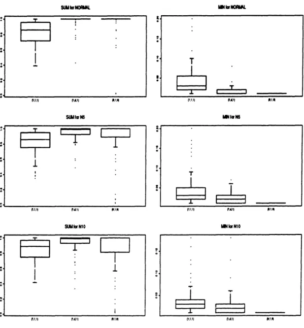
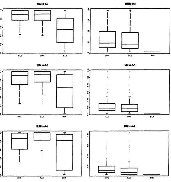
To deal with the chaining problem in real data, we combine kernel density estimation with the computation of minimal spanning trees to study the effect of density truncation on single-link partitions. New statistics are proposed to help decide on the best truncation level, leading to an improved version of the single-link method. Simulation studies show how these statistics perform with un:modal and bimodal densities. Finally, these tools are applied to two cluster,... xam-ples: One involves grouping several foods according to the nutrients they contain. The other is a market segmentation study, concerning an Atlanta manufacturer of prefabricated homes.

Thesis supervisor: Richard M. Dudley. Title : Professor of Mathematics.

ASYMPTOTIC AND 'COMPUTATIONAL PROBLEMS IN SINGLE-LINK CLUSTERING

by

ToUr' aCirb roizvvy v iC 6 7rp66Owv A6yo dKrairL ,

ro !ar 'iv / v a i iroAAcd acbrcv I?/Kdrpov,

Ktai mrD1 l• k•'tpa ci0),

dAA& rT& irore dpLO/6v kdrepov lp7rpooOcv CitrirmaL Trof) 6irELp ai'rwv 'EKarac 770ovLivaL;

This is exactly what the previous discussion requires from us: How is it possible for each of them

to be one and many at the same time

and how is it they do not immediately become Infinity but instead they first acquire a finite number

before each of them becomes Infinity? Plato, Philebus 19A.

Acknowledgements

New ideas rarely come out of nowhere and this work is no exception. The inspiration can often be traced back to the enlightening lectures I was fortu-nate to attend both at MIT and at Harvard University. Other contributions came in the form of informal discussions with a number of distinguished pro-fessors, friends and colleagues. For one or both of these reasons I feel I must mention, in particular, the names of: Dimitris Bertsimas, Kjell Doksum, Michael Economakis, Wayne Goddard, John Hartigan, Greta Ljung, Pana-giotis Lorentziadis, Walter Olbricht, Adolfo Quiroz, Helmut Rieder, David Schmoys, Hal Stern, Achilles Venetoulias and Jeff Wooldridge.

Special thanks are due to Peter Huber, Gordon Kaufman and Mark Matthews for reading this thesis and making several suggestions which re-sulted in substantial improvements. I must also thank Drazen Prelec for helping me find the data set used in chapter 7 and teaching me about mar-keting research. And, of course, I owe a lot to the continuous and patient guidance of my thesis supervisor, Richard Dudley. It would be impossible to mention the many ways in which he has contributed to this thesis but it suffices to say that, without him, I would have never brought this work to an end. I hope I haven't caused him too much aggravation during these years and I will always consider it an honor to be counted among his students.

The Department of Mathematics and the Sloan School of Management have provided financial support for my graduate studies at MIT. Richard Dudley, Gordon Kaufman and Phyllis Ruby were instrumental in securing it. Above all, however, I wish to thank my family for their support and love: my father for our lengthy discussions which influenced my way of thinking; my mother for taking care of every problem that occurred; my sister for keeping me in touch with reality over the years. These are the people that made this possible and to whom this work is dedicated.

Contents

1 Introduction

1.1 The clustering problem

1.2 Partitional methods .

1.3 Hierarchical methods .

1.4 Minimal spanning trees

2 Describing Hierarchies

2.1 A-hierarchies...

2.2 A-ultra-pseudometrics

2.3 Single-link hierarchies .

2.4 Single-link algorithms .

3.1 Distances as kernels of U-statistics 3.2 Clustered measures . . . . 3.3 Consistency of single-link distances

4 Asymptotics on the real line 4.1 Spacings ...

4.2 A central limit theorem . . . . 4.3 Measuring hierarchical structure .

5 Using the edges of the MST

5.1 Statistics related to the MST . . . 5.2 Upper bounds . . . . 5.3 Lower bounds . . . . 11 11 12 13 15 20 20 22 29 33 38 38 40 42 49 49 54 57 62 62 63 65 111 111

..

Iiir

6 Clustering under the Density Model 6.1 Chaining and breakdown points . . 6.2 Density clustered measures . . . . .

6.3

Estimating

7.1 Improving on single-link clustering 7.2 Food Data...

7.3 Market Segmentation Data . . . . .

. . . . . 72 . . . . . 74 . . . . 76 . . . . 83 96 . . . . . 96 . . . . 97 . . . . .100

List of Tables

6.1 Intervals for SUM, and MINn: Unimodal distributions. .... 85 6.2 Intervals for SUM, and MIN,: Uniform distributions. ... 85 6.3 Intervals for SUM, and MIN,: Bimodal distributions. ... 86 7.1 Nutrients in Meat, Fish and Fowl ... . . . . 98

List of Figures

1.1 The MST for a uniform on the unit square... 17

1.2 The MST for a mixture of two uniforms with disjoint support. 18 1.3 The MST for a contaminated mixture of two uniforms. .... 19

2.1 Single-link distances and the MST. ... 36

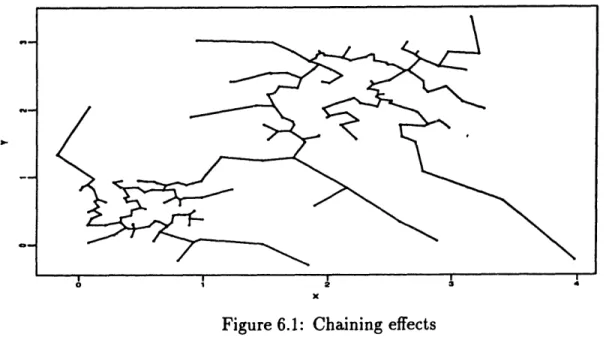
6.1 Chaining effects ... 73

6.2 An example of worst case performance ... 82

6.3 2-dimensional unimodal distributions ... 89

6.4 3-dimensional unimodal distributions ... 90

6.5 4-dimensional unimodal distributions ... 91

6.6 Uniform distributions on the unit cube ... 92

6.7 2-dimensional bimodal distributions ... 93

6.8 3-dimensional bimodal distributions ... 94

6.9 4-dimensional bimodal distributions ... .95

7.1 Chernoff faces for the food nutrient data ... 105

7.2 Choosing the best truncation level using T,•''1 (f, 6). ... 106

7.3 Single-link dendrogram for the food data... 107

7.4 The first two principal components for the Fabhus data. ... 108

7.5 The process T,",''(fn, 6) for the Fabhus data... 109

7.6 Single-link dendrogram for the 133 observations of the Fabhus data. .. . . . .. . . . . 110

7.7 The truncated Fabhus data projected on the same plane as before . . . .. 111

Chapter 1

Introduction

1.1

The clustering problem

The main problem of cluster analysis is summarized in [MKB79], page 360: Let xl,...,x, be measurements of p variables on each of n objects which are believed to be heterogeneous. Then the aim of cluster anal-ysis is to group these objects into g homogeneous classes where g is

also unknown (but usually assumed to be much smaller than n).

There is no shortage of proposed methods to tackle this problem. Detailed listings have been included in books and review papers such as, e.g., [Eve74], [Har75], [Gor81l], [Gor87], [JD88] and [KR90]. Very often, these methods are described by means of an algorithm. As it often happens with other non-parametric multivariate problems (see [Hub91]), the goal that the algorithm is trying to attain is not specified explicitly. This is partly c'ue to the lack of a universally accepted interpretation of the term homogeneous as used in the quote from [MKB79]. Such an intepretation would also amount to a de-scription of the properties of clusters and is, therefore, central to clustering analysis.

There are at least two widely used interpretations in the clustering litera-ture (see e.g. [Boc85] and [Gor87]). One describes homogeneity as uniformity on a compact and connected set G. Tests of this hypothesis can be based on the work of N. Henze ([Hen83]). A different approach has been taken by D. Strauss ([Str75]). The most important drawback is that these tests assume

that the set G is known. Without knowledge of G, we cannot account for the effect of the shape of G on the statistics used. A similar edge effect is recorded in the use of spatial processes in image processing (see e.g. [Rip88], chapter 3).

The other interpretation assumes the existence of a density f (with re-spect to Lebesgue measure) and equates homogeneity with unimodality of f. This leads us to the use of mode-seeking methods in order to specify the location of clusters (see e.g. [JD88], page 118). Note, however, that it is very difficult to find the modes of a density in d-dimensional space. In the one dimensional case, there has been some progress([Sil81], [HH85]). A sug-gestion for an extension of the one-dimensional method of [HH85] to higher dimensions is contained in [Har88].

A certain compromise between the two interpretations can be reached through the suggestion of J. Hartigan ([Har85]) to take clusters to be max-imally connected high-density sets, i.e. the connected components of the region {x E Rd : f(x) > c} for an appropriate c. It seems, therefore, that a search for clusters must use information about:

* where the observations lie and

* how densely they are packed together.

In fact, there have been suggestions ([Gil80]) which assume that a preliminary estimate of the location of each cluster is available (together with an estimate of the probability of the cluster) and proceed to find the observations that belong to that cluster through iterations. This, however, leaves the question of the global search for the location of the clusters open.

In the next two sections we intoduce the two main groups of clustering methods.

1.2

Partitional methods

The ambiguity of the terms homogeneous group or cluster makes it even more difficult to develop statistical inference for clustering. Some progress has been made in the area of partitional methods. These attempt to find a partition of the observations that optimizes a certain criterion. The main idea is to decide on the number of clusters before looking at the observations

and then try to minimize the within-cluster distances of these observations. Such methods (and related algorithms) go back to the work of Friedman and Rubin (see [FRb67]).

The most popular among them is the k-means method where the partition P = (C1, C2,..., Ck) chosen is the one that minimizes:

k n T(P) = Z Z(xj - ±) 2_1C,(Xj) i=1 j=1 where: U 1 lc,(zj)xj

X

i

I c

i l

Since the number of partitions of n observations into k clusters is:

(

(-I k-i(

)in

S(n,k) =k!

(the Stirling numbers of the second kind, see [Sta86], pages 33-34) an ex-haustive search is out of the question. Instead, iterative algorithms have been devised (see, e.g., [JD88], page 96 and [KR90], page 102).

Consistency of the k-means method is treated in [Har78], [Pol81] and, in a more general setting, in [CM88]. The asymptotic normality of the centers of the k-means clusters is proved in [Po182]. Another interesting question is the estimation of k. [But86] and [But88] treat this on rhe real line. More recently, [PFvN89] addressed the same problem in the rrliftivariate case.

1.3

Hierarchical methods

These methods use the observations to produce a sequence of n partitions

1, 22•, . ., •n (often refered to as a hierarchy of partitions) with the

proper-ties:

* 7₁ is the partition into n one-element clusters.

* Pi has n - i + 1 clusters of which n - i are the same as n -- i clusters in Pi-1 and the (n - i + 1)st cluster is formed by joining the remaining two clusters of Pi-1into one (i = 2, 3,..., n).

A class of such methods is based on defining a distance dc between

clus-ters. Then a general algorithm that produces the sequence (Pi, i

=

1,..., n}

is the following:

* P1 is the partition: {{zx}, {x2},..., ,n}}.

* Given P_-1, Pi is formed by finding the two clusters C, and C2 for

which: dc(Cl, C2) = min{dc(A, B), A,B E Pi-I} and join them into one cluster.

Popular choices for dc are:

dc(A, B) = min{d(x, y), x E A, y E B} and

dc(A,B) = max{d(x,y), x E A, y E B}

resulting into the single link and complete link methods respectfully (see, e.g., [KR90], page 47).

Hierarchical methods have certain advantages that make them popular. Some of them are:

* They describe the clustering structure of the data set without the need to prespecify the number of clusters we must look for. Choosing the number of clusters can be then based on inspection of the hierarchy of partitions. Note, however, that inspecting the partitions is not a trivial task for large data sets in high dimensions.

* The algorithm we just described needs O(n3_{) steps to form the} hierar-chy of partitions' compared to partitional methods that need iterarive algorithms to produce a single partition. Even worse, the work done to compute a partition into, say, three clusters cannot be used in cal-culating a partition into four or two clusters when using a partitional method.

* Identifying clusters is often a subjective decision. What some people may see as one cluster, some others might consider as two or more. It is

'Using the concept of reciprocal neighbors it is possible to form the hierarchy in O(n2) steps (see [LMW84], pages 128-129).

often a question of how fine a partition we want to find, that determines the answer. This feature of the clustering problem is best captured by hierarchical methods.

The hierarchical structure involved in these methods explains why there is so little work done on the asymptotics of hierarchical methods. The problem of consistency of single-link has been addressed in [Har81].

1.4

Minimal spanning trees in clustering

Tree methods are often used in nonparametric multivariate statistics (see e.g. [BFOS84] for classification and regression and [FRf79, FRf81] for the two-sample problem). In this thesis, we will make ample use of the minimal spanning tree (MST) on n points. This is simply any tree with vertices these n points that attains the smallest possible total length. Complete definitions of all the graph-theoretic terms involved will be given in Chapter 2. In general, an MST can be computed (by a variety of algorithms) in O(n2) time

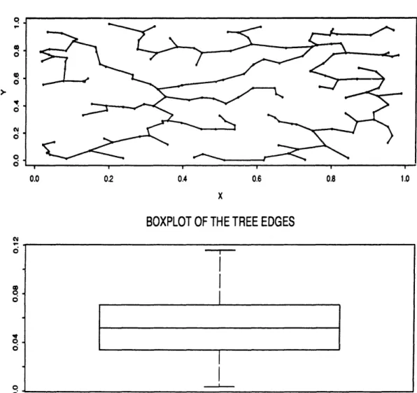
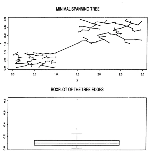
(see [Hu82] pages 28-29, [PS82] pages 271-279 or [NW88] pages 60-61). The close connection of the MST to clustering was pointed out in [GR69] and since then it is practically impossible to talk about single-link clustering without also talking about the MST. In Chapters 2,3,4 and 5, we will build on this connection to establish several asymptotic results about single-link. The connection is shown in the next examples. In Figure 1.1, we draw the MST for 160 observations drawn from the uniform distribution on the unit square and a boxplot for the edge lengths of this tree. As expected in this case, no edge stands out as significantly larger than the others. Compare that with Figure 1.2, where the MST and the corresponding boxplot is shown for a sample drawn from a mixture of two uniform distributions on disjoint squares. This time, the edge that connects the two squares is significantly longer than all others, indicating the existence of cluster structure. Removing this longest edge reveals the two clusters.

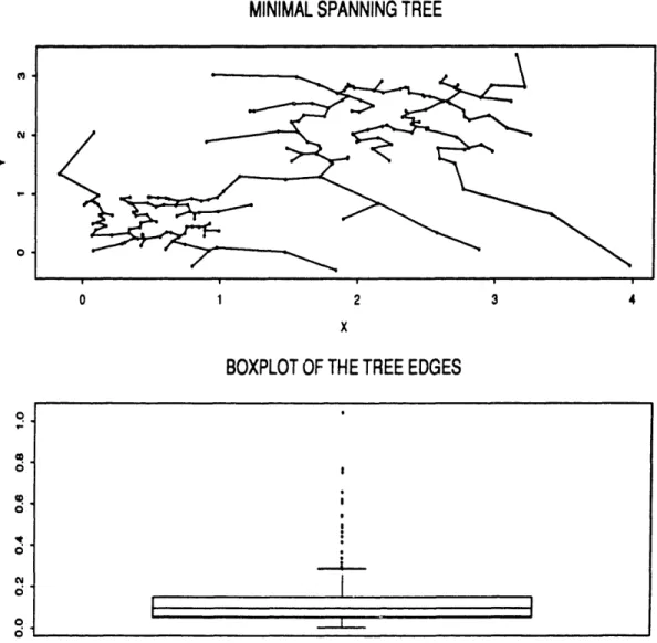
It may seem at this point that the use of the MST is all we need to solve the clustering problem described in Section 1.1. The next example shows that this is not the case at all. In Figure 1.3 we have the MST and boxplot for the same observations as in Figure 1.2, this time adding another 40 observations from a bivariate normal centered between the two squares.

Although the clustering structure is still clear to the human eye, the boxplot gives a very confusing picture. The additional observations form chains of observations through which the MST joins the two clusters without having to use a long edge. So, there is no significantly longest edge in this MST. In fact the longest edge is not connecting the two clusters but is rather caused by an outlier. This problem (appearing very often in real data) is called chaining. It seems, therefore, that some adjustments have to be made in order to be able to detect the cluster structure and discover the clusters in cases such as in Figure 1.3. This problem will be the object of Chapters 6 and 7.

MINIMAL SPANNING TREE

0.0 02 0.4 0.6 0.8 1.0

BOXPLOT

OF

THE

TREE EDGES

Figure 1.1: The MST for a uniform on the unit square.

IT

I

MINIMAL SPANNING TREE

BOXPLOT OF THE TREE EDGES

Figure 1.2: The MST for a mixture of two uniforms with disjoint support.

-MINIMAL SPANNING TREE

BOXPLOT

OF THE TREE EDGES

Figure 1.3: The MST for a contaminated mixture of two uniforms.

Figure 1.3: The MST for a contaminated mixture of two uniforms.

19

(W).

0*·

I

Chapter 2

Describing Hierarchies

2.1

A-hierarchies

Let A be a family of subsets of Rd

Definition 2.1.1 A partition P of a set S C Rd is a finite family Al, A2,..., A)} of non-empty subsets of Rd such that S = A1 U A2 U ... U A, and Ain Aj =

0

for i f j, 1 < i,j <r.

Definition 2.1.2 A partition P, of S is finer than a partition P2 of S (PA PndBB,...,B) i

VA E P2,3 r E N and BI, B2,

...

,

Br E Pi

such that:

A = BUB

U...UBr.

Definition 2.1.3 An A-clustering of a set S E Rd _{is a partition:}

C = {CI,C

,...,Cr}

Ci EA

c~nC

Definition 2.1.4 An A-hierarchy of a set S C Rd is a triple (7W, {Pik=0o, h) (or simply W" when there is no danger of confusion) where:

I. =PoUP U ... UPk where

* Pi is a partition of S, for 0 < i < k, * Po is an A-clustering of S,

* Pk =

{S}

and

* Pi-, < pifor 1 <i <k. 2. h : W- R+ such that:

* VA, B E : A C B = h(A) <h(B), * h(A) = 0 + A E G, VA E -.

Remark 2.1.1 VA E -, 3r E N and C1, C2,... , Cr E C such that: A = CUC2 U... U C,.

Remark 2.1.2 Let G(7", E) be the graph with vertices the sets of W and edges E, where:

E = {(A,B) : A,B E H-, 3i: A E P, B E P~i+, and A C B}. Then G(H-", E) is a tree with root S and leaves the sets of C.

Remark 2.1.3 VA Z B E 7"H one and only one of the following is true:

1. AnB=0,

2. ACBor 3. B cA.

2.2

A-ultra-pseudometrics

Definition 2.2.1 An ultra-metric (UPM) d on S C Rd is a pseudo-metric on S which, in addition, satisfies the inequality:

d(x, y) < max{d(x, z), d(z, y)},

Vx,y,

z E S.

Definition 2.2.2 An A-ultra-pseudometric (A-UPM) d on S C Rd is a UPM for which the family of sets:

{d-'(x,.)({O}), x E S} forms an A-clustering of S.

Lemma 2.2.1 Let d be an A-UPM on S C Rd and let:

C = {d-'(x,.)({0}), x E S}.

Then, VC1, C2 E C (C1 $ C2) and Vx, y1 E C, and x2, y2 E C2:

d(xl,

)

=

d(yl,

)

=

d(C

1

,C2) > 0

d(x

,y)

,

=

d(x

,

Y

)=

0.

Proof: Since xl,y1 E C1 = d-1(x,.)({0}) for some x E Ci: d(xi,x) = d(yl,x) = 0 = d(xl, yl) < d(xl, x) + d(x, yl) = 0 = d(xzl, yl) = 0. Similarly: d(x2, y2) = 0. Then: d(xi,x₂) < d(xl, y1) + d(y1,x2)

< d(xl, y,) _{+ d(y, y2) + d(y2, x} 2) = d(y₁, Y₂

Similarly: d(y,, y2) < d(x, x2). So:

d(xl,x 2) = d(yl, 2) = inf{d(z,,z2), zi E C1, z2 E C2} = d(C1, C). If d(C1, C2) = 0, then Ve > 0, 3~1 E C1, X2 E C2 : d(x, zz) < e. Suppose2

C1 = d-1(x,.)({0}) and C2 = d-'(y,.)({0}). Then:

d(x, y) < d(x, xi) + d(xi,X 2) + d(X2, y)

=

d(xi,x

) <

e.

d(x, y)

=

0

•

y E d-(z,.)({0}) = C,

C

As it turns out, A-hierarchies and A-UPMs are equivalent in describing hierarchical structure. The following theorem proves this in detail. The main idea used is taken from [Joh67].

Theorem 2.2.1 Let S C Rd, let H be the set of all A-hierarchies of S and U the set of all A-UPMs of S. Then, there is a map m : H U which is

1-1 and onto.

Proof: Let (7•, {Pi} =l, h) E H. Let C := Po. Consider the function: d• : Rd x Rd +

defined as follows: For every pair (x, y) E Rd x Rd let: L1,Y := {A E 7H: {x,y} C A}.

Since S E LE1,, L~, Y 00. Let A.,, = nAELX,,A. Because of Remark 2.1.3,

A,, fE 1H so we can define:

dn(x, y) := h(Ad,,). We must check that dn E U.

* Let x E S. Then 3 C, E C so that x E C,. Since A,,, E I7, we have (using Remark 2.1.1): C, C A3, ,. Also, by the definition of A ,,X:

A ,13 C C, . So:

A ,,, = C, =, dh(x,x) = h(A ,,, ) = h(C,) = 0 (by Definition 2.1.4).'

* du(x, y) = h(Ax,,) = dH (y, x).

* Let x, y, z E S. Then, z E A,z n A3,,. Because of Remark 2.1.3,

Ax,z C AY,, or Ay,' C A4_,1 . Let us assume that Ay,, C A,,z. Then:

h(Ay,z) < h(Ax,z) = du(y, z) 5 du(z, z). Also: {z,y} C A,,z so:

A₃,, C Ax,z = h(A₃,) < h(A_{, 3},z)

= d (x, y) < d&(x, z) = maxI{d,(x, z), du(y, z)}

< dH(X, z) + d,(y, z).

* Let x E S. Then again, let C, E C so that x E Cx.

Vy E C, : Ax,y = C3, = dn(x, y) = h(Cx) = 0.

Vy E S \ C",: C, C A,,Y but C3, : Ax,, = d (x, y) = h(Ax,,) > 0. So: dý'(x,.)({0}) = C, and

{dý'(x,.)0, x E S} = C,

So, du E U.

Conversely: Let d E U. Then:

C = {d-

1

_{(x,.)({}), x E S}}

is an A-clustering of S (Definition 2.2.2). We now define the following par-titions of S:

* Po:= C and VC E C: h(C):= O.

* Suppose Pi is defined and is equal to {A1, A2,..., A,,}. Let: s= minm d(At,AA).

Let

J :=

{j

Since at least two sets in Pi were joined into one in i+e, we have ri+l < ri. Finally, VB E Pi+1 \ Pi, let h(B) := si.

Since ri+l < ri, we will eventually reach a Pk with card(Pk) = 1. At this point the construction terminates and we let I- := Po U P, U ... U Pk.

We first need to show that Pi, 0 < i < k are partitions of S. If k = 0, this is obvious. Assume k > 0. In fact, we can show, by induction, that:

Pi = {A, A2,...,A,} is a partition and

diam(Az) < si, 1 < 1 < ri

* For i = 0, Po = _{C is a partition and, because of Lemma 2.2.1,}

diam(C) = 0, VC E C and so = mini<t<j<ro d(Ai, Aj) > 0. * Suppose Pi is a partition with diam(Ai) < si, 1 < I < ri.

Let B1, 1 < 1 < ri, be defined as above. Suppose 311, 12 such that

Bi, # Bi, and B f _{n Bt, # 0. That would mean 3Aj, 1 <}

_j:

d(Al, Aj) 5 si, d(A 1, Ai) < si

but

d(Ai, A12) > si. Let c < d(At,, A,2) - si. Then:

3xz, E Al,

xj

3x,

E

d(xt1, xX2) > d(Ait, A,₂) > si +

c/2.

By the induction hypothesis: d(xj, yj) < si. Then, applying the ultra-metric inequality:

d(xZ,,x1₂) < max{d(xz,,xj), d(xj, _x,2)} 5 _{max{d(xl,,xj), d(xj, yj), d(yj, x,2)}}

< max{si +

E/2,

+

contradicting d(xz,, ,12) > si + E/2. So,

V11, 12 :

Bl

B

B

nl

B12

$

0.

In addition: A, C Bt for 1 < I < ri so:

S = UtAt CUBI C S :- UtBB = S. So: i+1 = {Bt, 1 < 1 < r} is a partition.

Now, clearly, si+1 = minl<t<j<,r.+ d(B1, Bj) > si. As we just proved:

Vjl,j 2 E J1, (1 < 1 < ri) : d(Aj,,Aj2) < si.

By the induction hypothesis: diam(At) < si. So: diam(Bi) = diam(UEJE Aj)

= max{max diam(Aj), max d(

A,

yEJ1 310h, h J2EJ '

•

This completes the induction.

Using the fact that si+1 > si, it becomes obvious that the properties of the h function in Definition 2.1.4 also hold. So (H", {}fPi}o 0, h), as defined, is an A-hierarchy.

It remains to be proved that when the map m is applied to the A-hierarchy (7-1, {P7}o=₀, h) we just obtained, we get the original d back, i. e.

dw := m(-H(, {Pf,}o, h) = d.

We will prove that:

VX, y S: d (x, y) = d(x, y).

By definition: du(x, y) = h(Ax,,), where A.,, is the smallest set in 7H that contains both x and y. Let P; be the finest partition that contains Az,,.

We proceed by induction on i: * For i = 0, A,y E Po = C = {d-'(x,.)({0}), x E S}. Because A.,, E C: h(Ax,,) = 0 = dK(x, y) = 0. Because A,,, E {d-'(x,.)({0}), x E S}:

d(x, y)

=

0.

* Suppose d (x, y) = d(x, y) for all x, y E S such that: Ax,vI Po U T U ... U p'.

We will prove the same for A.,, E "Pi+ \1 i. Let Pi = {Af , A2,..., Ar,}. Then, for some 1, 1 < 1 < ri : A:,, = UjEJAj. Suppose:

x E Aj, y

E

By the definition of A.,, as the smallest set in N7 containing both x and

y:

Aj, n Aj, = 0. By the definition of si:

si:= min d(At, Aj)

1l<k<<r,

and that of Jr:

Jr :=

{j:

d(At, A,) 5

we have d(Aj,,Aj,) = si. Since Ax,s E •+I \ Pi, h(A',,) = si. Let

z E A•,. Then:

A,,, C Aj, C Ax,y

= h(Ax,z) 5 h(Aj,) 5 h(AX,I). Also A-,z C As, implies that:

Ax,z E Po U PI U... U P

and so, by the induction hypothesis dwt(x, z) = d(x, z). So: d(x,z) = dt(x, z) = h(A.,z)

< h(A,y) = si = d(As,, Aj,) inf d(u, w) d(, y)

uEA,,, eA, •, d(z, y)

But then d(x, y) = d(z, y). Otherwise, if, e.g.,

then the ultrametric inequality:

d(x,y) 5 max{d(z, y), d(x, z)}

would be violated. Similarly, for w E A,,:

AW,N C A , C = h(Aw,, ₎ < h(Ajy,)

and Aw,, C Aj, implies that:

A,, E Po U P, U.

Then, by the induction hypothesis: d(w, y) = du(w, y) = h(A,j,

< h(Ay,)

.. U PT.

< h(A1,V) = si

inf d(u, v) d(z,y)

UEAz ,vEAj. < d(z, w).

Then, again: d(z, y) = d(z, w). So:

d(x, y) = d(z,y) = d(z, w), Vz E Aj,, w E Xj,

. d(zx, y) = h(Ax,y) = si = d(Aj., Aj,)

= inf d(z, w) = d(x, y).

zEAJ,, wEAJ,

This concludes the proof of du = d and the proof of the theorem.

2.3

Single-link hierarchies

In what follows, we choose and fix a metric p on Rd that metrizes the usual topology. Definition 2.3.3 and Theorems 2.3.1 and 2.3.2 below are based on ideas in [LMW84], pages 143-144.

Definition 2.3.1 Let P be a partition of S C Rd. For A, B E 7, we define a path from A to B on P to be a finite sequence:

(A = Co, C1,..., Ck E B)

of sets Ci E P, 1 < i < k.

Definition 2.3.2 The size of a path (A = Co, C, ..., Ck = B) from A to B on P is defined to be:

max p(Ci-,, C,). l<i<k

Definition 2.3.3 Let C be an A-clustering of S C Rd. On S x S we define the function:

d'L : Sx S R+

as follows: For x, y E S let x E C, E C, y E C, E C. Then:

d'L(x,y) := min{s : 3 path

fromC,

Theorem 2.3.1 For any S C Rd and any A-clustering C of S, dcL is an A-UPM.

Proof:

1. For any C E C, the path (C, C) has size 0. So: Vx E S: dcL(, x) = 0.

2. To any path (Cx, = Co, C,...,Ck - Cy), there corresponds a path

(Cy 1 Ck, Ck-1, ..* , - C) of the same size. So: dSL(x,y) = dCL(y,x).

3. Let x, y, z E S. Let us fix, for the moment, a path (C,,..., C,) of size sl and a path (C.,..., C,) of size 82. Then, the path:

(C., ... , C,, ... , CY)

has size max{s

,,s

}. So dcgL(X,y) < max{s,s8

}. Taking the minimum

over all paths from C, to C, and all paths from C, to C, we get:

dcL(z,y) _ max{dcL(x,z), dL(z,y)},

the ultrametric inequality.

4. Finally:

Vy E C, : dCn(x, y) 5 p(C,C,,)

=

0

so C, C dcL.'(x,.)( {0}). If, however, y E S \ C,, then all paths from C, to C, include a first step from C, to some C E C, C

$

C0

dc-'

1

_(x,.)({0})

₌

_C,

_{x {d~L-'(z,.)({0}), x E S} = C,}

Definition 2.3.4 The A-hierarchy (H7, {P,}i=o, h) = m-l(dcn) correspond-ing to dcL through the map m of Theorem 2.2.1 is called the scorrespond-ingle-link hierarchy with respect to C.

The choice of dc (among other UPM that can be based on the same A-clustering C) might seem arbitrary. The following theorem gives a reason. Theorem 2.3.2 Let S C Rd and C an A-clustering of S. Let D(C) be the set of all A-UPM d such that:

*

{d-'(x,.)((0}),

X

E S} = C.

Then:

Vd E D(C), V, E S : d(x, y) 5 dSCL(x,y) < p(x,y).

Proof:

* An obvious path from C, to C, is just (Ci, C,) with size p(C,, C,) <

p(x, y). Taking the minimum over all paths from C, to C,:

dcL(x, y) < p(x, y).

* Let r = card(C). Fix x, y E S. Let x E C E C and y E CE C. A path from C, to C, of the form (C,,..., C,,..., Cp,..., C ,) cannot have size less than the same path without the inner cycle (C,,..., C,). So it is safe to assume that the optimal path from C, to C, has, at most, r vertices. Let

(C,

-

Co, CI, Ct,..i, Ck

ECy)

be such a path. Choose c > 0.

For 0 < i < k - 1, choose yi E Ci and xi+, E Ci+, so that:

p(Xi+,, y;)

<

p(C, Ci+i) +

E.

For any d E D(C) the ultrametric inequality implies that:

d(x,y) < max{d(x, k), d(xk, y)}

< max{d(x, yk-1), d(yk-1, Xk), d(xk, y)}

< max{d(z, yo), d(yo, 2x), d(xl, yl),..., d(xk,y)}

= max d(yi-l,xi)

I<i<k

because distances within the clusters Co,..., Ck are 0 (Lemma 2.2.1). Then, by assumption:

d(x,y) 5 _1<i<kmax p(yi-.1,zi)

< max p(Ci-1, Ci) + rc < max p(C-i<k ,Ci) + r

Letting e

'

d(x, y) < max p(Ci-

, Ci)

=

size(Co, CI,..., Ck).

Since this is true for any path from C, to C, with < r vertices, it is also true for the optimal path. So d(x,y) 5 dCL(x, y).

This completes the proof. o

2.4

Single-link algorithms

The definition and treatment of single-link hierarchies and distances in the previous section is somewhat different from the traditional approach found in the literature. In that traditional treatment, a finite set S = {x1,x2,... , x,}

of observations is specified (possibly the values Xi(w), X2(w),..., X,(w) of

iid random variables) and distances dSL(xi, xj) are defined only on the finite set S. Notice, however, that this can now be considered a special case of single-link distances.

Definition 2.4.1 Let A, be the class of singletons zx}, z E Rd. Let S = {x1,x 2,.. .,,n} be a finite subset of Rd. Then Cs = {{xz}, 1 < i < n} is an

.A,-clustering of S.

We define the (classical) single-link distance on S x S as:

dSL(xi, (x) = dsCL (x, xj)_, 1 < i,j 5 n.

Remark 2.4.1 As the following example shows, dSL(x, y) does not depend only on X and y but on the whole set S:

On the real line, let p be the usual metric. Then:

d' 5)(0, 5)

=

p(O, 5)

=

5

but

Finding efficient algorithms to compute single-link distances (and thus

form single-link hierarchies as in Theorem 2.2.1) is going to be our next

priority. A very popular method (providing an algorithm that computes

the matrix {dSL(xi, x)} ,= in just O(n

_{) steps is based on the minimal}

spanning tree. As in the previous section, we will present this concept in the

more general setting of dsL distances on S x S, with respect to a certain

clustering C of S.

Remark 2.4.2 Because of Lemma 2.2.1, computing dCL on S x S is reduced

to computing the matrix:

{dcL(C,,

C,)

We will now need the following elementary terminology from graph the-ory.

Definition 2.4.2 Given a finite graph G = (V, E) with vertices in V and edges in E:

1. a tree T = (VT, ET) is a subgraph of G (i.e. VT C V and ET C E) which is connected and contains no cycles,

2. a spanning tree is a tree for which VT = V,

3. a weight function on G is a function w : E 4 R+ ,

4. the weight of a tree T is w(T) = ZeEET w(e), and 5. a minimal spanning tree is any tree To for which:

w(To) = min{w(T), T is a spanning tree of G}.

Remark 2.4.3 In general, there can be several minimal spanning trees as in the following example:

and Let:

E, = {{1,2}, {3, 1},

E2 = {{1,2}, {2, 3}},

Es = {{2,3}, {3, 1})}.

Then T1 = (V, E1), Tz = (V, E2) and Ts = (V, E3) are all

trees of G.

Remark 2.4.4 If T is a spanning tree of G = (V, E), then there exists a unique path from v to u along edges of T any edge more than once.

Proposition 2.4.1 Let C be an A-clustering of S C Rd.

plete graph G with vertices in V = C. define:

minimal spanning

for every v, u E V, that does not use

Consider the

com-,w: E R+: e = {Ci, C}

l

p(C,, Cj),

for Ci, Cj E C. Let T be a minimal spanning tree of G. Let p7z(Ci, Cj) be the unique path from Ci to Cj along edges of T that does not use any edge more than once. Define:

dT(C,, Cj)

=

size(pr(Ci, Cj).

Then:

dT(C;, Cj) = dCL(Ci, Ci).

Proof: Clearly dT(Ci, Cj) Ž> dcL(Ci, Cj) (see Definition 2.3.3). Suppose dT(Ci, Cj) > dcL(Ci, C,) _{for some Ci, Ci E C. Then, there is a path from Ci}

to Cj whose size is less than size(pT(Ci, Cj)). Let:

size(pT(Ci, Cj)) = p(Ck, C),1 Ck, C1i C.

Let:

be the path with size <

p(Ck, CI).

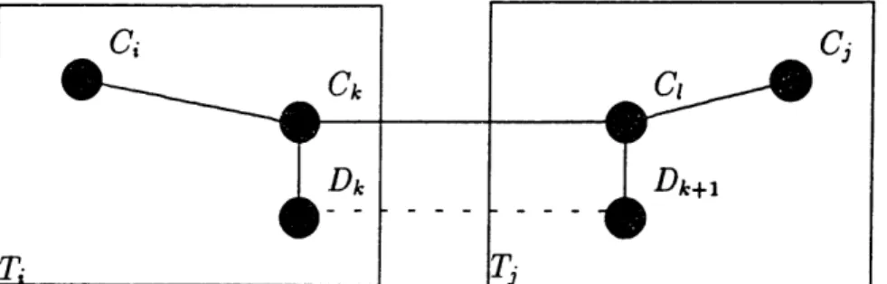
Removing the edge (Ck, CI) from the tree T, divides T into 2 trees T, = (Vi, E,) and T, = (Vj, E,) with V n Vf = 0 and Ei n Ej = 0, such that C, E Vi and Cj E V, (see Figure 2.1). However, the path

(Ci =Do, D1, ... , D, = Cj)

connects C; to Cj, so 3Dk, with Dk E Ti, Dk+1 E Tj and p(Dk,Dk+I) <

p(Ck,CI). So, substituting the edge (Ck, C) with (Dk,Dk+l) gives a new spanning tree T' with w(T') < w(T), a contradiction. So dT(Ci, Cj) =

dL (C,, C,).

o

The last proposition implies that the computation of the matrix:

{dcs(C,, Cj)}, 1 < i,j < n

reduces to the computation of:

{dT(C,,Cj)}, 1

5

for some minimal spanning tree T. The next step now is to provide an efficient algorithm for computing minimal spanning trees. Several such algorithms exist, proposed by Florek et al., Kruskal and Prim. Details are provided in [LMW84]. Here we will give a version of Prim's algorithm as found in [Hu82].

ALGORITHM: Let C = {C1,C2, -.. , Ck} be an A-clustering of S. Let

rij = p(Ci, Cj), 1 < i,j < k.

Step 0: Let V:= {C}), E:= 0. Let tj := rlj, 2 < j < k.

Step 1: If V = {Ci,,C,₂,..., Ci}, 1 < < k, let t,÷, = min{tj, Cj V}. Find h, 1 < h < 1 such that ii,=, = ri,,i,l,.

Include Ci,+, in V and (C,, C,I,+) in E.

Step 2: If Il+l = k, let T = (V, E) and stop.

Otherwise, VCj , V, t, := min{tj, rji,,, }. Continue with step 1.

The fact that the resulting graph T is a minimal spanning tree is a conse-quence of the following two lemmas proved in [Hu82] (page 28).

Lemma 2.4.1 If p(Ci, Cj,) = minj;ip(Cj, Cj) then there exists a minimal spanning tree containing the edge (Ci, Cj,).

Lemma 2.4.2 If T = (V, E) is a tree, known to be part of a minimal span-ning tree, and:

B3C E V, C2 E C\ V: p(C, C2)= min p(C, D)

CEV, DEC\V

then there exists a minimal spanning tree including the edge (C1, C2) and having T as a subtree.

Remark 2.4.5 Both step 1 and step 2 of the algorithm described require O(k2_{) operations, so this is an O(k}2_{)-complexity algorithm. (More details on}

that can be found in [Hu82], as above).

We now have the necessary tools to treat single-link hierarchies defined on a set S, not necessarily finite. In the next chapter, we will use these tools to explore the asymptotic behavior of single-link hierarchies, based on an iid sample.

Chapter 3

Consistency

3.1

Distances as kernels of U-statistics

Up to now, we have treated clustering -as a data analytic problem, we have

not introduced probability measures and we have not made any

distribu-tional assumptions concerning the observed data. In this chapter, we will

be introducing a model, appropriate for the study of hierarchical clustering

methods, so that we can study consistency of the method described in the

previous chapter. To achieve this goal we will make use of the equivalence

of hierarchies and ultrametrics that we have proved (Theorem 2.2.1).

Be-cause of this result, we can rely exclusively on the study of ultrametrics for

a complete description of the behavior of the corresponding hierarchies.

Suppose that d is a distance on Rd. Let P be a Borel probability measure

on Rd and let:

X1, X2,..., X, iid - P.

We will soon need to study statistics of the form:

Z2F Fd(Xj,,X3 ).

i=1 j=1

Fortunately, such statistics are special cases of U-statistics (of order 2) with

kernel d and their asymptotic properties are well understood.

Definition 3.1.1 Let P be a Borel probability measure on Rd and let:

be a measurable, symmetric real function. Let Xt, X2,..., X, iid ^ P and

define:

1

n

Un := Un(XI, X2, X ... ,Xn)

_(n

n

₂

₎

₌

_jfi

₊

X).

We call U, the U-statistic (of order 2) with kernel h.

U-statistics have been studied by Hoeffding (see [Hoe48]) and Halmos (see [Hal46]). They generalize the sample mean and in fact, Halmos has proved that when Ep(h') < oo then U,n is the unbiased estimator of Ep(h) with smallest variance. However, here we are more interested in the asymptotic properties of U,. A detailed list of asymptotic results on U-statistics is included in [Ser80], chapter 5. A law of large numbers for U, is provided by the following:

Theorem 3.1.1 Let P, h, U, be defined as in Definition 3.1.1. Then, if

Ep(hl) < oo we have :

Un(Xi,

X2,

X,)

EP(h)

almost surely.

Proof: The result was established by Hoeffding but an easier proof based on the reversed martingale structure of U, is given by Berk in [Ber66]. 0

In addition, we have the following central limit theorem for U-statistics: Theorem 3.1.2 Let P, h, U, be defined as in Definition 3.1.1 and define:

h Rd -4 R : x h(xz,y)P(dy)

and V(h1) := Varp(hi(X1)). Then, if Ep(h') < o0: '(V'(U, - Ep(h))) ') N(O, 4V(h1)).

Proof:

The original proof was given by Hoeffding in [Hoe48]. In this form,

the theorem is proved in [Dud89j, pages 337-339.

Remark 3.1.1 Notice that a distance d is a symmetric function which is

equal to 0 on the diagonal. Therefore, the difference between:

in2

i=l j=1

and:

₁

_{n n}

XE ) (3.2)

is just the difference between the scaling factors:

1

1

- and

n;

_{n(n - 1)}

Because of this, we will have no difficulty applying the asymptotic results for

(3.2) (such as Theorem 3.1.1 and Theorem 3.1.2) to (3.1).

Remark 3.1.2 There is also no difficulty in extending Theorem 3.1.1 and

is the k x k covariance matrix:

V(h,) := Covp(hu,(X,),..., hlk(X1)).

3.2

Clustered measures

Let us begin our study of the asymptotics of single-link distances by

ex-amining consistency. In this and the following chapters, p will denote the

euclidean distance on Rd unless otherwise noted.

Definition 3.2.1 A Borel probability measure P on Rd will be called

A-clustered if there exists an A-clustering of supp(P). If A is the class of compact and connected sets, then P will be simply called clustered.

Remark 3.2.1 For a general class of sets A and an A-clustered measure P, there might exist more than one A-clustering of supp(P). For an example, consider A = { finite subsets of Rd} and take P to be any probability measure with 1 < card(supp(P)) < oo.

The next proposition shows that such ambiguity is avoided in the case of clustered measures:

Proposition 3.2.1 Let P be a clustered measure in Rd. If C is a clustering of supp(P), then:

C = {C, E supp(P)}

where C , is the unique connected component of supp(P) containing z. Proof: Let C = {A₁,A2,..., A,}. Take x E Ai for some i : 1 < i < r. Since Ai is connected:

Ai CCz.

By Definition 2.1.3: Ak n Am = Ak n Am = 0 for 1 < k < m < r. So, there

exist open sets Uk, U,,,:

Ak C Uk, AmC

Um,

Ukn Um =.

Then:

C- C supp(P) = Ax U A2 U... U A, C U1U U2 U... U U,.

Since C_ is connected, there is a unique j, 1 <

j

$

C, C Ui n supp(P) = Ai. Therefore, C, = Ai. We conclude that:

C = {C,, x E supp(P)}.

Remark 3.2.2 Proposition 3.2.1 shows, in particular, that supp(P) has a finite number of connected components.

We can now give the following definition:

Definition 3.2.2 Let P be a clustered measure. Then, C(P) will denote the unique clustering of supp(P).

3.3

Consistency of single-link distances

Let P be a clustered measure in Rd and let X1, X2,..., X, iid - P. If P" denotes the empirical measure:

1n

P,(w)

:= -

x,(Y)

then Pn is a clustered measure with:

C(Pn) = S, := {{Xi}, 1 < i < n for all w.

Therefore, given X 1,X 2,... Xn iid - P, we can define two different single-link distances. One is ( P) that is defined on supp(P) x supp(P) with respect to the clustering C(P) (Definition 2.3.3). The other is d( P")

defined on S, x S, with respect to the clustering C(P,) (Definition 2.3.3 but also Definition 2.4.1). Therefore, both distances are defined on S, x Sn, although only dC( P) is observable.

What follows is the main result of this chapter. It shows that, as n goes to co, dC(q P") converges (uniformly on the sample) to dC P).

Theorem 3.3.1 Let P be a clustered measure in Rd and let: X1,X 2,..., Xn lid - P.

If Pn denotes the empirical measure, then, for n E N and 1 < i,j 5 n, we define: _{An(X, Xj) = d(Pn)(Xi, Xj) - dC( P)(Xi, Xj).}

Then:

* An(Xi,Xj);> 0 a.s. for 1 < i,j < n and * limn-oo max_<i,<in An(Xi, Xj) = 0 a.s..

Proof: Let C(P) = {C1, C2,..., C,}. If r = 1 then let 6 := oo, otherwise: 6:= min _{p(Cj, C).}

Because of the definition of a clustering (Definition 2.1.3) and the fact that p metrizes the usual topology: 6 > 0. Choose and fix e such that 0 < e < 6. Since supp(P) = Ur=xCi is compact, there exists a finite number (say k(e)) of open balls with radius e/4 covering supp(P). Let B be such a cover. Consider now the following lemma:

Lemma 3.3.1 Let P,C,A,,e,B and k(e) be defined as above. If, for some n, all k(e) balls in B contain at least one observation each, then:

max A,(Xi, Xj) < e.

<_i,j<n

Proof: (of Lemma 3.3.1) First note that:

dsC( P)(Xi, Xj) dsC( P)(Xi, Xj), 1 < i,j < n.

Indeed, if Xi E Ci, Xj E Cj, then to every path from Xi to X, on C(P,), there corresponds a path from Ci to C, on C(P) having edges smaller or equal to the corresponding edges of the path on C(P,). So:

A,(X,, xj) > o.

On the other hand:

dSC ()(Xi, Xj) = min{s : 3 path from Ci to Cj with size s}.

Let:

(Ci _{Do, DI, ... , Dk E Cj)}

be one of the paths that achieve the above minimum. We can now construct a path from Xi to Xj on C(P,) with size < dC ( P)(Xi, Xi) + e, using the assumption of the lenima.

To do that, we begin by choosing observations:

Xi 7 X X''o, Xii, l I,, .X., XI, : X such that:

* Xi, X!j E Di, 0 <_1 < k and

* p(Xi,_,,Xi, ₎ _ p(DI-II,DI) + e.

We can do this as follows:

For 1 such that 1 < 1 < k, 3a'-1 E DI-1, at E DI such that p(a'l-,a,) = p(DI-1, Di) (because the sets D1 and Dt1_ are compact). Then 3BBL 1, Bt E B such that a'_1 E B-_1 and at E B1. Finally, using the assumption of the lemma:

3XB'1 e B'_1 and X;, E Bt. Then:

p(X,_,, X,) _ p(X',_,,

al-

) + p(a_-

,

at) +

p(at,

X,,)

< C/2 + p(Di-1, DI) + e/2

5 c + dr P(Xi,xj).

We must now complete the path from Xi to X, by inserting paths from Xi, to Xf, of size < e for 0 < 1 < k. Notice that, thanks to our initial choice of f, no ball B E B intersects more than one of the clusters C1, C2,..., C,.

Concentrating now on the cluster Dr under consideration, we define:

* B1 to be the subcover of 8 covering Dr,

* S1 to be the set of observations contained in Dr (these include, in

par-ticular Xi, and Xi,),

* Sx to be the set of observations from St reachable from X with paths of size < e for X E St,

* Ex to be the set of balls from B1 containing observations from Sx and

* Ex := UBEexB (an open set). Note that:

*

Si

= UxEs,Sx,

* B1 = UxEsEx (since all balls contain observations) and

Also, for X, Y E SI, either: or

Sx n Sy =

Ex

n Ey =

Ex n Ey = 0.

VX, Y E St : Ex = Ey = Sx = Sy.

In particular, Sx,1 = SxI and so there exists a path from X;, to Xf, of size < e. These path segments (for 0 < 1

<

size s with: s < max{,, + dsC(P)(X, X) } = + ds P)(Xi,Xj) So:

.j(P")(-x<,,Xj) < +

dj

(

Xxx)

i, <

Smax A, (Xi, X) <

C

proving the lemma.

Now, to complete the proof of Theorem 3.3.1 note that we can always assume that all k(e) balls of the cover have positive probability. If some of them have probability 0, we can discard them and still be able to cover supp(P) with the rest. Let p := minBES P(B) > 0.

Now, using Lemma 3.3.1:

Pr(max 6s(X;, X,) > e) < Pr(3 B E B containing no observations) < Pr(B is empty) BEB < [1 - P(B)I" BEB

<

k)(-

p)".

since p > 0. So, by the Borel-Cantelli lemma:

Pr(lim sup A') = 0 =j max A,(Xi, X) -- a.s.

as n -+ co.

The last theorem provides us with the means to study statistics based on single link distances:

Definition 3.3.1 Let P be a clustered measure in Rd and let:

C(P)

:=

{C1,

C2,

C

,

C,}.

Since the length of the longest edge of any minimal spanning tree on C(P)

must be equal to max1<i,<,n dC( P)(Ci, C) (see Proposition 24.1), we can

define:

* M(P) := the length of the longest edge of any minimal spanning tree of C(P) and

Remark 3.3.1 M(P) is the largest single-link distance on C(P) while D(P)

is the average single-link distance on C(P).

Theorem 3.3.2 Let P be a clustered measure on Rd and let

X1,X2,... ,Xn lid , P.

If Pn is the empirical measure then, as n --+ oo:

M(P,) D(Pn)

--- M(P) a.s. and

-- + D(P) a.s.

Proof:

The result for M(P) is obtained by direct application of

as n -+ 00.

M(P,) - M(P) < max A(X, X) ---- 0 a.s. "3

The case of D(P) needs some more work. Since 0 < dC( ) < p on supp(P) (Theorem 2.3.2) and supp(P) is compact:

D(P) =

y)P(dx)P(dy) < oo.

Then, the U-statistic with kernel dP): 2 U := (

n(n - 1) -ZdsCLI(X i<j

,Xi)

U,, - D(P) a.s. (3.3)

Then:

ID(P,)

-

D(P)I

• I'EdsClP"n)(X,,Xj)

+

I

EdLc

1,3

+ IU. - D(P

<

max

IdC

Xj)-d

(Xi, X)l

-<i,j<n

1 1

+

2

n(n -1)I

+

jU. - D(P)I

< _{-- <ij<n}max An(Xi, Xj)O

0 20 Oa.s.

E

dsCj

PI(Xi,

Xj)

+ -

Un| +

jUn

- D(P)

P'(Xi iXj) - Un I

Chapter 4

Asymptotics on the real line

4.1

Spacings

The fact that the statistic D(P,) introduced in Chapter 3 exhibited simi-larities to a U-statistic, encourages us to attempt a more detailed study of the asymptotic behavior of D(PB). More specifically, one would hope that D(P,) behaves similarly to:

SCds(

P)(X,

y)Pn(dz)Pn(dy)

which cannot be observed (since P is not known) but which is a U-statistic. Notice that, to prove consistency for D(P,), we used the fact that:

lim max A,(Xi, Xj) = O a.s.

(Theorem 3.3.1). To prove asymptotic normality, we will need something stronger, namely:

max A,(Xi, Xj) = o,(1/ ).

As it will turn out, this is only true when d = 1.

Clustering on the real line has been studied in the literature: [Har78] has studied the asymptotics of k-means clustering on the real line and more recently [But86] and [But88] have dealt with optimal clustering on the real line. Hartigan has also proved set-consistency for the single-link method on the line ([Har81]) and showed that set-consistency fails in higher dimensions.