Bounds on Multithreaded Computations
by Work Stealing
by
Warut Suksompong
MASSACHUSETTS INSTIaUTE OFTECHNOLOGYJUL 15 2014
LIBRARIES
Submitted to the Department of Electrical Engineering and Computer Science in partial fulfillment of the requirements for the degree of
Master of Engineering in Electrical Engineering and Computer Science at the Massachusetts Institute of Technology
June 2014
@2014 Massachusetts Institute of Technology. All rights reserved.
Signature
redacted
Author ...-...
Department of Electrical Engineering and Computer Science
May 23, 2014
Certified by ...
Signature redacted
Charles E. Leiserson, Professor of Computer Science and Engineering Thesis Supervisor
Bounds on Multithreaded Computations by Work Stealing
by
Warut Suksompong
Submitted to the Department of Electrical Engineering and Computer Science on May 23, 2014, in partial fulfillment of the requirements
for the degree of
Master of Engineering in Electrical Engineering and Computer Science
Abstract
Blumofe and Leiserson [6] gave the first provably good work-stealing work scheduler for mul-tithreaded computations with dependencies. Their scheduler executes a fully strict (i.e., well-structured) computation on P processors in expected time T1/P + O(To), where T denotes the minimum serial execution time of the multithreaded computation, and T. denotes the minimum execution time with an infinite number of processors.
This thesis extends the existing literature in two directions. Firstly, we analyze the number of successful steals in multithreaded computations. The existing literature has dealt with the number of steal attempts without distinguishing between successful and unsuccessful steals. While that approach leads to a fruitful probabilistic analysis, it does not yield an interesting result for a worst-case analysis. We obtain tight upper bounds on the number of successful steals when the computation can be modeled by a computation tree. In particular, if the computation starts with a complete k-ary tree of height h, the maximum number of successful steals is E' 1(k - 1) (h).
Secondly, we investigate a variant of the stealing algorithm that we call the localized
work-stealing algorithm. The intuition behind this variant is that because of locality, processors can
benefit from working on their own work. Consequently, when a processor is free, it makes a steal attempt to get back its own work. We call this type of steal a steal-back. We show that under the "even distribution of free agents assumption", the expected running time of the algorithm is
T1/P + O(TOO
lg
P). In addition, we obtain another running-time bound based on ratios betweenthe sizes of serial tasks in the computation. If M denotes the maximum ratio between the largest and the smallest serial tasks of a processor after removing a total of O(P) serial tasks across all processors from consideration, then the expected running time of the algorithm is T1
/P+O(TM).
Acknowledgements
First and foremost, I would like to thank my thesis supervisor, Prof. Charles E. Leiserson. Charles is a constant source of great advice, and his guidance has been instrumental in shaping this thesis. It has truly been a pleasure working with him.
I would also like to thank Tao B. Schardl. Tao provided helpful comments for most of the work in this thesis, and his positive attitude to things has been a source of inspiration for me. I never found it boring to work on research problems with Tao.
In addition, I would like to thank MIT for offering a variety of resources and serving as a world in which I can learn best.
Thanks also to my friends, near and far, for helping me with countless things throughout my life.
Contents
1 Introduction 9
2 Definitions and Notations 13
3 Worst-Case Bound on Successful Steals 17
3.1 Setting . . . . 18
3.2 Binary Tree and One Starting Processor ... 20
3.3 Rooted Tree and One Starting Processor ... 25
3.4 Rooted Tree and Many Processors . . . . 30
3.5 Properties of Potential Function . . . . 36
4 Localized Work Stealing 45 4.1 Setting . . . 46
4.2 Delay-Sequence Argument . . . . 48
4.3 Amortization Analysis . . . . 52
4.4 Variants . . . . 56
Chapter 1
Introduction
Scheduling multithreaded computations is a complicated task, with a number of heuristics that the scheduling algorithm should follow. Firstly, it should keep enough threads active at any given time so that processor resources are not unnecessarily wasted. At the same time, it should maintain the number of active threads at a given time within reasonable limits so as to fit memory requirements. In addition, the algorithm should attempt to maintain related threads on the same processor so that communication across processors is kept to a minimum. Of course, these heuristics can be hard to satisfy simultaneously.
The two main scheduling paradigms that are commonly used for scheduling multithreaded computations are work sharing and work stealing. The two paradigms differ in how the threads are distributed. In work sharing, the scheduler migrates new threads to other processors so that underutilized processors have more work to do. In work stealing, on the other hand, underutilized processors attempt to "steal" threads from other processors. Intuitively, the migration of threads occurs more often in work sharing than in work stealing, since no thread migration occurs in work stealing when all processors have work to do, whereas a work-sharing scheduler always migrates threads regardless of the current utilization of the processors.
authors point out the heuristic benefits of the work-stealing paradigm with regard to space and communication.
Since then, many variants of the work-stealing strategy has been implemented. Finkel and Manber [13] outlined a general-purpose package that allows a wide range of applications to be implemented on a multicomputer. Their underlying distributed algorithm divides the problem into subproblems and dynamically allocates them to machines. Vandevoorde and Roberts [22] described a paradigm in which much of the work related to task division can be postponed until a new worker actually undertakes the subtask and avoided altogether if the original worker ends up executing the subtask serially. Mohr et al. [19] focused on combining parallel tasks dynamically at runtime to ensure that the implementation can exploit the granularity efficiently. Feldmann et al. [12] and Kuszmaul [18] applied the work-stealing strategy to a chess program, and Halbherr et al. [15] presented a multithreaded parallel programming package based on threads in explicit continuation-passing style. Several other researchers [2, 3, 4, 5, 7, 9, 11, 17, 20, 23] have found applications of the work-stealing paradigm or analyzed the paradigm in new ways.
An important contribution to the literature of work stealing was made by Blumofe and Leiser-son [6], who gave the first provably good work-stealing scheduler for multithreaded computations with dependencies. Their scheduler executes a fully strict (i.e., well-structured) multithreaded com-putations on P processors within an expected time of T1/P + O(T.), where T is the minimum
serial execution time of the multithreaded computation (the work of the computation) and T, is the minimum execution time with an infinite number of processors (the span of the computation.) Furthermore, the scheduler has provably good bounds on total space and total communication in any execution.
This thesis extends the existing literature in two directions. Firstly, we analyze the number of successful steals in multithreaded computations. The existing literature has dealt with the number of steal attempts without distinguishing between successful and unsuccessful steals. While that approach leads to a fruitful probabilistic analysis, it does not yield an interesting result for a worst-case analysis. We obtain tight upper bounds on the number of successful steals when the computation can be modeled by a computation tree. In particular, if the computation starts with
a complete k-ary tree of height h, the maximum number of successful steals is Z 1(k - 1)i(h).
Secondly, we investigate a variant of the stealing algorithm that we call the localized
work-stealing algorithm. The intuition behind this variant is that because of locality, processors can
benefit from working on their own work. Consequently, when a processor is free, it makes a steal attempt to get back its own work. We call this type of steal a steal-back. We show that under the "even distribution of free agents assumption", the expected running time of the algorithm is
T1
/P
+ O(T.Olg
P). In addition, we obtain another running-time bound based on ratios betweenthe sizes of serial tasks in the computation. If M denotes the maximum ratio between the largest and the smallest serial tasks of a processor after removing a total of
O(P)
serial tasks across all processors from consideration, then the expected running time of the algorithm is T1/P+0(TOM).The remainder of this thesis is organized as follows. Chapter 2 introduces some definitions and notations that we will use later in the thesis. Chapter 3 explores upper bounds on the number of successful steals in multithreaded computations. Chapter 4 provides an analysis of the localized
Chapter 2
Definitions and Notations
This chapter introduces some definitions and notations that we will use later in the thesis.
Binomial Coefficients
For positive integers n and k, the binomial coefficient (n) is defined as = if n > k
k k k! (n - k)!
and
(n)
= 0 if n < k. A usual interpretation is that(n)
gives the number of ways to choose kobjects from n distinct objects. This interpretation is consistent when n < k, since there is indeed
no way to choose k object from n distinct objects in that case. The binomial coefficients satisfy Pascal's identity [10]
(n) = (n-1) +
(
)
(2.1)k k k - 1
for all integers n, k > 1. One can verify the identity directly using the definition.
Figure 2.1: The complete binary tree CBT(4) of height 4
Figure 2.2: The almost complete ternary tree A CT(2, 3, 3) of height 3 and root branching factor 2
CBT(4) is shown in Figure 2.1.
For k > 2, h > 0, and 1 < b < k - 1, let ACT(b, k, h) denote the almost complete (or complete) k-ary tree with b- kh leaves, where the root has b children, and every other node has 0 or k children. For instance, the tree ACT(2, 3,2) is shown in Figure 2.2. By definition, we have CBT(h) =
ACT(1, 2, h). Also, the tree ACT(b, k, h) is complete exactly when b = 1.
For any tree T, let ITI denote the size of the tree T, i.e., the number of nodes in T.
Computation Trees
Consider a setting with P processors. Each processor owns some pieces of work, which we call
serial tasks. Each serial task takes a positive integer amount of time to complete, which we define
as the size of the serial task. We model the work of each processor as a binary tree whose leaves are the serial tasks of that processor. We then connect the P roots as a binary tree of height
lg
P,We define T as the minimum serial execution time of the multithreaded computation (the work of the computation), and To as the minimum execution time with an infinite number of processors (the span of the computation.) In addition, we define T.' as the height of the tree not including the part connecting the P processors of height
lg
P at the top or the serial task at the bottom. InChapter 3
Worst-Case Bound on Successful
Steals
The existing literature on work stealing has dealt extensively with the number of steal attempts, but so far it has not distinguished between successful and unsuccessful steals. While that approach leads to a fruitful probabilistic analysis, it does not yield an interesting result for a worst-case analysis. In this chapter, we establish tight upper bounds on the number of successful steals when the computation can be modeled by a computation tree. In particular, if the computation starts with a complete k-ary tree of height h, the maximum number of successful steals is j=1 (k - i)().
The chapter is organized as follows. Section 3.1 introduces the setting that we consider through-out the chapter. Section 3.2 analyzes the case where at the beginning all the work is owned by one processor, and the computation tree is a binary tree. Section 3.3 generalizes Section 3.2 to the case where the computation tree is an arbitrary rooted tree. Section 3.4 generalizes Section 3.3 one step further and analyzes the case where at the beginning all processors could possibly own work. Finally, Section 3.5 elaborates on a few properties of the potential functions that we define to help with our analysis.
3.1
Setting
This section introduces the setting that we will consider throughout the chapter.
Consider a setting with P processors. Each processor owns some pieces of work, which we define as serial tasks. Each serial task takes a positive integer amount of time to complete, which we define as the size of the serial task. We model the work of each processor as a tree whose leaves are the serial tasks of that processor.
We are concerned with the worst-case number of successful steals that can occur throughout the execution of all serial tasks, as a function of the structure of the trees of the P processors. That is, given the structure of the trees of the processors, suppose that an adversary is allowed to choose the sizes of the serial tasks in the trees. Moreover, whenever a processor finishes its current work, the adversary is allowed to choose which other processor this processor should steal from.
In this setting, it is not an interesting question to ask about the worst-case number of steals overall, whether successful or not. Indeed, the adversary can choose to make almost all steals unsuccessful, and thus the worst-case number of steals is governed by the maximum amount of work among the P processors. But as we are concerned only with successful steals here, the adversary cannot benefit from making steals unsuccessful.
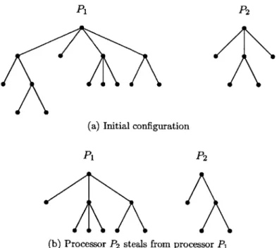
Before we begin our analysis of the number of successful steals, we consider an example of an execution of work stealing in Figure 3.1. There are two processors in this example, P and P2, and the initial structure of the trees corresponding to the two processors are shown in Figure
3.1(a). Three successful steals are performed, yielding the tree structures in 3.1(b), (c), and (d) respectively. In this example, the maximum number of successful steals that can be performed in the execution is also 3. Observe that we have not chosen the sizes of the serial tasks in the example. Nevertheless, we will show in the next section that for any sequence of steals, such that the one in Figure 3.1, the adversary can choose the sizes of the serial tasks so that the execution of work stealing follows the given sequence of steals.
P1 P2
(a) Initial configuration
P1 P2
(b) Processor P2 steals from processor P1
P1 P2
(c) Processor P, steals from processor P2
P1 P2
0 0
(d) Processor P steals from processor P2
3.2
Binary Tree and One Starting Processor
In this section, we establish the upper bound on the number of successful steals in the case where at the beginning, all the work is owned by one processor, and the computation tree is a binary tree. We first prove a lemma showing that we only need to be concerned with the structure of the trees, and not the size of the serial tasks. Then, we define a potential function to help with establishing the upper bound, and we derive a recurrence relation for the potential function. The recurrence directly yields an algorithm that computes the upper bound in time O(ITIn). Finally, we show that the maximum number of steals that can occur if our configuration starts with the tree CBT(h) is
i=1 (
Recurrence
Recall that in our setting, the adversary is allowed to choose the sizes of the serial tasks in the trees. Intuitively, the adversary wants to make sure that when a steal occurs, the trees not involved in the steal are working on serial tasks that are large enough so that they cannot finish the tasks yet. We formalize this intuition in the following lemma.
Lemma 1. Fix the structure of the binary trees belonging to the P processors. Given a sequence
of steals performed on the trees, the adversary can choose the sizes of the serial tasks in such a way that when the execution proceeds, the steals that occur coincide with the given sequence of steals. Proof. First, the adversary chooses every serial task to be of size 1. Consider the steals in the given
sequence, one by one, and imagine an ongoing execution. Suppose that the next steal dictates that processor Pi steal from processor P. The adversary waits until Pi finishes its remaining serial tasks, and meanwhile increases the sizes of the serial tasks belonging to all trees except Pi, if necessary, to ensure that those trees do not finish before Pi. Then the adversary dictates that Pi steal (successfully) from P. In this way, the adversary can implement the given sequence of
steals. 5
Lemma 1 tells us that in order to establish the upper bound on the number of successful steals, it suffices to consider only the structure of the given trees and determine a maximum sequence of
steals.
Suppose that we are given a configuration in which all processors but one start with an empty tree (or one serial task-it makes no difference to possibilities of sequences of steals), while the exceptional processor starts with a tree T. How might a sequence of steals proceed? The first steal is fixed-it must split the tree T into its left and right subtrees, T and T,. From there, one way to proceed is, in some sense, to be greedy. We obtain as many steals out of T as we can, while keeping Tr intact. As such, we have P -1 processors that we can use to perform steals on T, since the last processor must maintain Tr. Then, after we are done with T, we can perform steals on Tr using all of our P processors. This motivates the following definition.
Definition 2. Let n > 0 be an integer and T a binary tree. The nth potential of T is defined as
the maximum number of steals that can be obtained from a configuration of n + 1 processors, one of which has the tree T and the remaining n of which have empty trees. The nth potential of T is denoted by 4P(T, n).
If we only have one processor to work with, we cannot perform any steals, hence 4(T, 0) = 0
for any tree T. Moreover, the empty tree EMPT and the trivial tree with a single node TRIVT cannot generate any steals, hence D(EMPT, n) = 4D(TRIVT, n) = 0 for all n > 0.
In addition, the discussion leading up to the definition shows that if a binary tree T has left subtree T and right subtree Tr, then for any n > 1, we have
4D (T, n) 1 1+ 4(T, n - 1) + <Db(Tr, n).
By symmetry, we also have
In the next theorem, we show that this inequality is in fact always an equality.
Theorem 3. Let T be a binary tree with more than 1 node, and let T and T be its left and right subtrees. Then for any n > 1, we have
<b(T, n) = 1 + max{<b(T, n - 1) + <b(T, n), <b(T, n - 1) + <b(T, n)}.
Proof. Since we have already shown that the left-hand side is no less than the right-hand side, it
only remains to show the reverse inequality.
Suppose that we are given any sequence of steals performed on T using n processors. As we have noted before, the first steal is fixed-it must split the tree T into its two subtrees, T and
Tr. Each of the subsequent steals is performed either on a subtree of T or a subtree of T (not
necessarily the left or right subtrees of T or T.) Assume for now that the last steal is performed on a subtree of T. That means that at any particular point in the stealing sequence, subtrees of
T occupy at most n - 1 processors. (Subtrees of T may have occupied all n processors at different
points in the stealing sequence, but that does not matter.) We can canonicalize the sequence of steals in such a way that the steals on subtrees of T are performed first using n - 1 processors,
and then the steals on subtrees of Tr are performed using n processors. Therefore, in this case the total number of steals is at most 1 + <b(T, n - 1) + <b(T, n).
Similarly, if the last steal is performed on a subtree of T, then the total number of steals is at most 1 + <(Tr, n - 1) + 4(Ti, n). Combining the two cases, we have
<D (T, n) <; 1 + max{<4D(T, n - 1) + 4D (Tr, n), 4Db(Tr, n - 1) + <b (T, n)},
which gives us the desired equality.
Algorithm
When combined with the base cases previously discussed, Theorem 3 gives us a recurrence that we can use to compute <b(T, n) for any binary tree T and any value of n. But how fast can we compute
the potential? The next corollary addresses that question. Recall from Chapter 2 that ITI denotes the size of the tree T.
Corollary 4. There exists an algorithm that computes the potential 4(T, n) in time O(ITIn).
Proof. The algorithm uses dynamic programming to compute 4(T, n). For each subtree T' of T
and each value 0 < i < n, it computes 4(T', i) using the recurrence given in Theorem 3. There
are O(lTIn) subproblems to solve, and each subproblem takes 0(1) time to compute. Hence the running time is O(ITIn).
Complete Binary Trees
An interesting special case is when the initial tree T is a complete binary tree, i.e., a full binary tree in which all leaves have the same depth and every parent has two children. Recall from Chapter 2 that CBT(h) denotes the complete binary tree with height h. The next corollary establishes the potential of CBT(h). Recall also from Chapter 2 that
()
0 if a < b.Corollary 5. We have
4(CBT(h),n)=
()
+()
+... + ()Proof. The case h = 0 holds, since
b(CBT(O), n) = = 0.
i=1
The case n = 0 holds similarly. Now suppose h, n > 0. Since the two subtrees of CBT(h) are
Using Pascal's identity (Equation 2.1), we have =1+ 4(CBT(h -1), n- 1) + ((CBT(h -1), n) fh 1) "~n -1 ) n -= h 0 1) + ( 1) i h 1 i=n= (h - 1) +h-1) n= -(h=1 as desired. 5
For fixed n, 4(Tbin,perf,hn) grows as O(hn). Indeed, one can obtain the (loose) bound
Z
(h) <
h
n
for h, n > 2, for example using the simple bound
(h) h(h - 1) ... (h-i ) h(h
-and then computing a geometric sum.
We have established the upper bound on the number of successful steals in the case where at the beginning, all the work is owned by one processor, and the computation tree is a binary tree. In fact, this configuration is used in usual implementations of the work-stealing algorithm, and as such the analysis presented in this section suffices. Nevertheless, in the next sections we will generalize to configurations where the work can be spread out at the beginning and take the form of arbitrary rooted trees as well.
3.3
Rooted Tree and One Starting Processor
In this section, we consider a generalization of Section 3.2 to the configuration in which the starting tree is an arbitrary rooted tree. The key observation is that we can transform an arbitrary rooted tree into a "left-child right-sibling" binary tree that is equivalent with respect to steals. With this transformation, an algorithm that computes the upper bound in time
O(ITIn)
follows. Finally, we show that the maximum number of steals that can occur if our configuration starts with the treeACT(b, k, h)
isEn 1(k
- I)i(h) + (b -1) E
_~ (k - 1)i(h).We assume that nodes in our tree can have any number of children other than 1. The reason is that if a node has one child, it is not clear how a steal should proceed. We still maintain the assumption that at the beginning all work is owned by one processor. So far, we have not specified whether when processor P steals from processor P1 it should steal the left subtree or the right subtree. In fact, it must steal the subtree that P is not working on. Up to now, this distinction has not mattered in our analysis, because the processors are symmetric: when one tree breaks into its two subtree, it does not matter which processor has which subtree. In this section, however, we will use the convention that a processor works on serial tasks in its right subtree, and when another processor steals from it, that processor steals the left subtree.
With this convention, we can define how a steal is performed on arbitrary rooted trees. Suppose that processor P steals from processor Pj, and assume that the root node of P has m children.
If m > 2, then P steals the leftmost subtree, leaving the root node and the other m - 1 subtrees of P intact. On the other hand, if m = 2, then the usual steal on binary trees is applied. That
is, P steals the left subtree, leaving P with the right subtree, while the root node disappears. An example of an execution of work stealing on rooted trees is shown in Figure 3.2. In this example, the root node has four children, and therefore the steal takes away the leftmost subtree and leaves the remaining three subtrees intact. This definition of stealing in rooted trees is not arbitrary. It
P1 P2
(a) Initial configuration
P1 P2
(b) Processor P2 steals from processor P
Figure 3.2: Example of an execution of work stealing on rooted trees
Algorithm
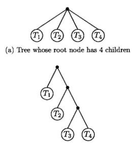
The key to establishing the upper bound in the case of arbitrary rooted trees is the observation that the problem can in fact be reduced to the case of binary trees, which we have already settled in Section 3.2. Indeed, one can check that a node with k children is equivalent (with respect to stealing) to a left-child right-sibling binary tree [10] of height k - 1. For instance, the complete
quarternary tree of height 1 is equivalent to a left-child right-sibling binary tree of height 3, as shown in Figure 3.3.
With this equivalence, one can transform any rooted tree into a binary tree by transforming each node with more than two children into a left-child right-sibling binary tree on its own. The transformation is shown in Figure 3.4. Therefore, we can use the same algorithm as in the case of binary trees to compute the maximum number of successful steals, as the next theorem shows. Recall from Chapter 2 that IT denotes the size of the tree T.
Definition 6. A node in a rooted tree is called a singleton node if it has exactly one child. Theorem 7. Let T be a rooted tree with no singleton nodes. There exists an algorithm that
(a) The complete quarternary tree of height 1
(b) Left-child right-sibling binary tree representation of the tree in (a)
Figure 3.3: Rooted tree and left-child right-sibling binary tree
T1 T2 T3 T4
(a) Tree whose root node has 4 children
T3 T4
computes the potential <D(T, n) in time
O(ITIn).
Proof. We transform T into a binary tree according to the discussion leading up to this theorem,
and apply the algorithm described in Corollary 4. The transformation takes time of order ITI, and the algorithm takes time of order ITIn. 0
Complete k-ary Trees
As in our analysis of binary trees, an interesting special case is the case of a complete k-ary tree, i.e., a full k-ary tree in which all leaves have the same depth and every parent has k children. Moreover, we also determine the answer for almost complete k-ary trees. Recall from Chapter 2 that for k> 2 h > 0, and 1 < b < k - 1, A CT(b, k, h) denotes the almost complete (or complete)
k-ary tree with b -kh leaves.
Theorem 8. Fork> 2,h>O, and 1<b< k-1, we have
<D(A CT(b, k, h), n) = (k - 1)() + (k - 1)2(h) + -+ (k - 1)n(h))
+ (b - 1) (h)+ (k - 1) ()+ --- + (k - 1)n-1
n n-i
Z(k - 1)'(7 + (b - 1) (k - 1)1).
i=1 i=O
written as A CT(k, k, h) for h > 0. Indeed, we have <D(A CT(1, k, h + 1), n) =(k - 1) ( 1 + (k - )2 +1 + - -- + (k - n) =(k - 1) (()+ (h)+ (k - 1) 2 (()+ () + .. . + (k - 1)n +() (k - 1)() + (k - 1)2) -- + (k - 1)n + (k -1)
(
+() + (k -1) + -+ (k -1)n1 h = <(A CT(k, k, h), n),where we used Pascal's identity (Equation 2.1).
We proceed to prove the formula. The case b - kh = 1 holds, since both the left-hand side and the right-hand side are zero. The case n = 0 holds similarly. Consider the tree ACT(b, k, h), where
b -kh > 1 and 2 < b < k. Using the consistency of the formula that we proved above, it is safe to
represent any nontrivial tree in such form. Now, the recurrence in Theorem 3 yields
4(ACT(b, k, h), n) = 1 + max{<I(A CT(b - 1, k, h), n) + 4(A CT(1, k, h), n - 1),
<I(A CT(b - 1, k, h), n - 1) + 4(A CT(1, k, h), n)}.
Letting A =<D(A CT(b - 1,k, h),n)+<b(A CT(1,k, h),n - 1) and B = <D(A CT(b - 1,kh),n
-1) + <D(A CT(1, k, h), n), we have n A = E(k -(i=1 n =((k -i=1 )i W1(h) n-1 + (b - 2) (k i=O n-1 + (b - 1) (k> i=0 ()) n-1 - 1 +(k - 1)i h i=1 -
))-and
(n1n-2 nh
B = (k - 1) i()+ (b - 2) (> - 1) i()+ E(k - h)
=1i=O \/ i=1 = A - (b - 2)(k - 1)n-1 < A. Therefore, we have <D(A CT(b, k, h), n) = 1+ A = (k - 1)' + (b - J)>( - 1) , i=1 i=O as desired. 0
We have established the upper bound on the number of successful steals in the configuration with one processor having an arbitrary rooted tree at the beginning. In the next section, we generalize one step further by allowing any number of processors to own work at the beginning.
3.4
Rooted Tree and Many Processors
In this section, we consider a generalization of Section 3.3 where the work is not limited to one processor at the beginning, but rather can be spread out as well. We derive a formula for computing the potential function of a configuration based on the potential function of the individual trees. This leads to an algorithm that computes the upper bound for the configuration with trees T1, T2,. ..., Tp
in time O(P3 + P(IT1I + IT21+ ... + ITpI)). We then show that for complete k-ary trees, we only need to sort the trees in order to compute the maximum number of steals. Since we can convert any computation tree into a binary tree, it suffices throughout this section to analyze the case in which all trees are binary trees.
Formula
Suppose that in our configuration, the P processors start with trees T1, T2,..., Tp. How might a
sequence of steals proceed? As in our previous analysis of the case with one starting processor, we have an option of being greedy. We pick one tree-say Ti-and obtain as many steals as possible out of it using one processor. After we are done with T1, we pick another tree-say T2-and obtain
as many steals as possible out of it using two processors. We proceed in this way until we pick the last tree-say Tp-and obtain as many steals out of it using all P processors.
We make the following definition.
Definition 9. Let T1, T2,..., T,, be binary trees. Then <b(T1, T2,..., T,) is the maximum number
of steals that we can get from a configuration of n processors that start with the trees T1, T2,... ,T.
Note that we are overloading the potential function operator 4. Unlike the previous defi-nition of <b, this defidefi-nition does not explicitly include the number of processors, because it is simply the number of trees included in the argument of <D. It follows from the definition that
<D(T1, T2,. . .., Tn) = <b(To(1), Ta(2),..., Ta(n)) for all permutations o of 1, 2,..., n. From the discussion leading up to the definition, we have
<b(T1, T2,. .. , Tp) <P(Ta(l), 0) + <b(Ta(2), 1) +... + 4(T,(p), P - 1)
for any permutation a of 1,2,... , P. It immediately follows that
D(T1, T2, .. ,Tp) aESPmax (<b(T,(1), 0) + <b(Ta(2), 1) + ... + '(T,(p), P - 1)),
where Sp denotes the symmetric group of order P, i.e., the set of all permutations of 1,2,... , P. The next theorem shows that this inequality is in fact an equality.
Proof. We have already shown that the left-hand side is no less than the right-hand side, hence it
only remains to show the reverse inequality.
Suppose that we are given any sequence of steals performed on T1, T2,..., Tp using the P
processors. Each steal is performed on a subtree of one of the trees T1, T2, ... , Tp.
Assume without loss of generality that the last steal performed on a subtree of T occurs before the last steal performed on a subtree of T2, which occurs before the last steal performed on a subtree
of T3, and so on. That means that at any particular point in the stealing sequence, subtrees of T
occupy at most i processors, for all 1 < i < P. (Subtrees of T may have occupied a total of more than i processors at different points in the stealing sequence, but that does not matter.) We can canonicalize the sequence of steals in such a way that all steals on subtrees of T are performed first using one processor, then all steals on subtrees of T2 are performed using two processors, and
so on, until all steals on subtrees of Tp are performed using P processors. Therefore, in this case the total number of steals is no more than 4D(T, 0) + D(T2, 1) + ... + <D(Tp, P - 1).
In general, let
a
be the permutation of 1, 2,. .., P such that the last steal performed on a subtreeof T(1) occurs before the last steal performed on a subtree of T(2), which occurs before the last steal performed on a subtree of T(3), and so on. Then we have
4)D(T1, T2,., TP) ! <(D(TM(1), 0) + (D (To(2), 1) + . + <D (TU(P), P - 1).
Therefore,
4D(T1, T2, ... ,Tp) 5 max (<D(T.(1), 0) + 4D(Ta(2), 1) + ... + 4D(To(P), P - 1))
which gives us the desired equality. [
Algorithm
Now that we have a formula to compute < (T1, T2, ... , Tp), we again ask how fast we can compute
Corollary 11. There exists an algorithm that computes the potential 4(T1,T2,...,Tp) in time
O(P3 + P(ITI + IT2
1
+ . .. + ITpI)).Proof. The potentials 4(Ti,j) can be precomputed by dynamic programming in time O(P(ITi + IT2
1+
... +ITpI))
using the algorithm in Corollary 4. It then remains to determine the maximumvalue of 4(To(1), 0) + 4(T,(2), 1) + .. .+ 4D(T(p), P - 1) over all permutations a of 1, 2,... , P. A
brute-force solution that tries all possible permutations a of 1, 2,.. ., n takes time O(P!). However, our maximization problem is an instance of the assignment problem, which can be solved using the classical "Hungarian method". The algorithm by Tomizawa [21] solves the assignment problem in
time O(P3). Hence, the total running time is
O(P
3 + P(ITiI + IT2
1+
... +ITpI)).
Complete Trees
It is interesting to ask whether we can do better than the algorithm in Corollary 11 in certain special cases. Again, we consider the case of complete trees. In this subsection we assume that the
P processors start with almost complete (or complete) k-ary trees (defined in Chapter 2) for the
same value of k. The case where the values of k are different across different processors is harder to deal with, as will be explained in the next section.
Suppose the processors start with the trees A CT(bi, k, h1), A CT(b2, k, h2),. . ., A CT (bp, k, hp),
where 1 < bi, b2, . . ., bp 5 k -1. We may assume without loss of generality that b, -kh, < b2 -kh2 < ... < bp - khp. Intuitively, in order to generate the maximum number of successful steals, one might want to allow larger trees more processors to work with, because larger trees can generate more steals than smaller trees. It turns out that in the case of complete trees, this intuition always works, as is shown in the following theorem.
Theorem 12. Let b1 -kh, < b2 -kh2 < ... < bp -khp. Consider almost complete (or complete) k-ary trees ACT(b1,k,h1),ACT(b 2,k,h2),...,ACT(bp,k,hp). We have
there exist two consecutive positions
j
andj
+1
such that bj -khj > bj+1 kh3+1. We show that wemay exchange the positions of the two trees and increase the total potential in the process. Since we can always perform a finite number of exchanges to obtain the increasing order, and we know that the total potential increases with each exchange, we conclude that the maximum potential is obtained exactly when the trees are ordered in increasing size.
It only remains to show that any exchange of two trees bi - kh3 and bj+1 -khi+1 such that bj -khi > bj+l - khi+1 increases the potential. Denote the new potential after the exchange by N and the old potential before the exchange by 0. We would like to show that N > 0. We have
N
-O =(k- ) + (bj -_1 (k j-1 1)
+ (k - 1) h ) + (bk+1 - 1)Z(k - 1)i h3+)
i=1 i=
j-1 j-2
+ (i=1 EZ(k - 1)1 + (by - 1)
Z(k
i=O - )j-1
- (k - 1) h3+) + (bj+1 - 1) (k - 1) hi+)
i=1 i=
- (k - () + (b - 1)(k - 1)1
G-(k - 1) h)+1 (bj - 1)(k - 1) 1 +
We consider two cases.
bj+1-We have N - 0 = (k - 1)j .hj + (bj - 1)(k - 1)j-l( j1 - (k - 1)i
(h)
- (bj+1 - 1)(k - 1)31(- h)
= (bj - 1)(k - 1)j-1 j1 - (bj+1 - 1)(k - 1)j- ~ = ((bj - 1) - (bj+1 - 1))(k - 1)j- i- h1 = (bj - bj+1)(k - 1)-1 > 0, since bj > bj+j. Case 2: hj > hj+1 -We have N- O= (k - 1) + (bj - 1)(k - 1)j-1 - (k - 1) hj+1) (bj+ - 1)(k - 1)j~1(j+1
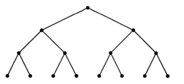
>(k - 1)i j (k - 1)j (hj+1 - (bj+1 - 1)(k - 1)jl hj+l (k - 1)j hi) - (k - 1)j (hj+i) - (k - 1)(k - 1)j_1 hj+1 (k - 1)j -(k - i) ((h+) + j+1 =(k - 1)j j - (k - 1)j h+l + 1) = (k - 1)j hi) _ (h+ + 1) > 0,Figure 3.5: The complete binary tree CBT(3) of height 3
It follows from Theorem 12 and Corollary 11 that in the case of complete k-ary trees, one only needs to sort the trees with respect to their size in order to compute the potential. It follows that the running time of the algorithm is bounded by the running time of sorting, which is
O(P lg
P).We have established the upper bound on the number of successful steals in a configuration with all processors having an arbitrary rooted tree at the beginning by defining a potential function. The next section takes a closer look at some properties of our potential function.
3.5
Properties of Potential Function
In the previous sections, we have shown recurrence formulae for computing the potential function, as well as closed-form formulae for certain special cases, such as complete trees. In this section, we shed more light on properties and computations of the potential function. We provide counterexamples to two conjectures of 'nice" properties of the potential function, and we give alternative ways of computing the potential function.
Tree Ordering
Theorem 12 raises the natural question of whether we can do better than the algorithm in Corollary
11 in general. In particular, one might expect that we can always order the trees according to their
size as in Theorem 12 and compute the potential of the configuration. This is not necessarily true, however, as the following example shows.
Consider the complete binary tree CBT(3) of height 3 (Figure 3.5) and the complete ternary tree ACT(1, 3, 2) of height 2 (Figure 3.6). Suppose that we have a configuration of 5 processors
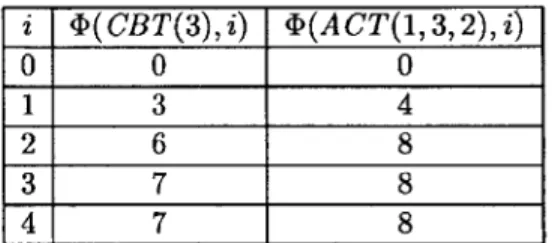
Figure 3.6: The complete ternary tree A CT(1, 3, 2) of height 2 i <D(CBT(3), i) <D(A CT(1, 3, 2), i) 0 0 0 1 3 4 2 6 8 3 7 8 4 7 8
Table 3.1: Potentials of the trees 4(CBT(3),i) and <D(ACT(1,3,2),i)
(P = 5), three of which start with the tree CBT(3), and the remaining two of which start with the
tree ACT(1, 3, 2). Thus the maximum number of successful steals in this configuration is given by the potential <D(CBT(3), CBT(3), CBT(3), ACT(1, 3,2), ACT(1, 3,2)).
To calculate this potential, we first calculate the potentials <D(CBT(3), i) and 4(ACT(1, 3,2), i)
for 0 < i < 4. Since both trees are complete k-ary trees, the formula given in Theorem 8 applies.
The results are shown in Table 3.1.
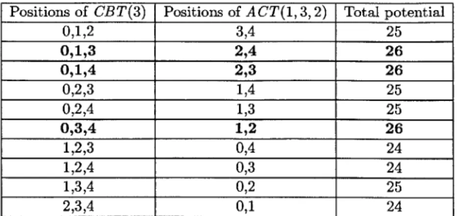
We are now ready to compute <D(CBT(3), CBT(3), CBT(3), ACT(1, 3,2), ACT(1, 3,2)). We do that by considering all possible ordering of the trees. The results are shown in Table 3.2.
The orderings that yield the maximum potential have the trees CBT(3) in positions {0, 1, 3},
{0, 1, 4}, and {0, 3, 4}. None of these orderings provide an order between the trees CBT(3) and A CT(1, 3,2). Indeed, such orderings would require CBT(3) to be in either positions
{0,
1, 2} orpositions
{2,
3, 4}. This example shows that an inherent order between trees does not exist even when the trees are complete k-ary trees, if the trees have different values of k.Positions of CBT(3) Positions of ACT(1, 3,2) Total potential 0,1,2 3,4 25 0,1,3 2,4 26 0,1,4 2,3 26 0,2,3 1,4 25 0,2,4 1,3 25 0,3,4 1,2 26 1,2,3 0,4 24 1,2,4 0,3 24 1,3,4 0,2 25 2,3,4 0,1 24
Table 3.2: Calculation of the potential <b(CBT(3), CBT(3), CBT(3), A CT(1, 3,2), A CT(1,3, 2))
i ID(CBT(3),i) + 4(ACT(1,3,2),i+ 1) <D(ACT(1,3,2),i) + <(CBT(3),i+
1)
0 4 3
1 11 10
2 14 15
3 15 15
Table 3.3: Placement of two trees in consecutive positions
Monotonicity
Another interesting question to ask is the following: Given two trees, T and T2, and two positions,
is it always optimal to place one tree in the "higher" position and the other tree in the "lower" position? If the answer is affirmative, it could lead to a way of simplifying the calculation of the potential in Theorem 12.
Unfortunately, the answer is negative, and it remains negative even when we limit our attention to two consecutive positions. The same two trees CBT(3) and ACT(1, 3,2) once again provide a counterexample.
As shown in Table 3.3, we cannot determine which tree to place in the "higher" position without considering the positions themselves. There exists a position in which it is optimal to place ACT(1, 3,2) in the higher position (i = 0, 1), a position in which it is optimal to place
CBT(3) in the higher position (i = 2), and a position in which both options are equally optimal
A follow-up question is whether this "turning point" at which the optimality changes from one
tree being in the higher position to the other tree being in the higher position happens at most once. In this example, there is only one turning point from i = 1 to i = 2. If this statement is true in general, it could yet lead to a way to simplify the potential computation. We do not know the answer to this question.
Alternative Computation Methods
In this subsection, we provide alternative ways to compute the potential 4D(T, n) that are equivalent
to the method given in Theorem 3.
As an example, consider the binary tree T given in Figure 3.7, and suppose that we wish to compute 4D (T1, 2). In general, when we compute the potential 4 (T, n), the recurrence formula given
in Theorem 3 chooses one of the two branches and decreases the second argument in the potential function to n - 1 for that branch, while maintaining the second argument in the potential function
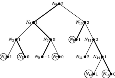
as n for the other branch. In the tree in Figure 3.7, we choose one of the two branches for each non-leaf node, and the chosen branches are bolded. The number next to each node indicates the value of n corresponding to that node.
For example, the bottom-right node N15 has value 0, because the way down from the root node
to it contains two bolded branches. On the other hand, node N1 1 has value 2, because the way
down from the root node to it contains no bolded branches. It is easy to see that the label of any node is no more than n, and it can also be negative (as in the case of node N5 here.)
We make the following definition.
Definition 13. For a binary tree T, let F(T) denote the set of all the ways to choose one of the
two branches for each internal (i.e., non-leaf) node of a binary tree T.
If a tree T contains k internal nodes, then
IP(T)I
= 2k. Indeed, each internal node allows aN4 N10 2
N2 1N6 0 N9 I Nl 2 2
N1 1 N3 0 N5 -1N7 0 N11 2 N14 1
N13 1 N15 0
Figure 3.7: Breakdown of potential calculation in an example binary tree
Theorem 14. Let n > 0. For each fixed -y E F(T), label each node with n subtracted by the number of chosen branches on the path from the root node to it, and let f1(-y) denote the number of internal
nodes with positive label. Then 4D(T, n) = maxyEr(T) fl
(7).
Proof. In the recurrence in Theorem 3, the only place where a potential arises is every time we invoke the recurrence on an internal node, and a potential of exactly 1 arises. Therefore, for fixed
y, a potential of 1 arises exactly when an internal node has a positive label (since we can invoke the
recurrence on it). Since < (T, n) is simply the maximum obtained over all possible ways to choose
branches, we have the desired result. 5
For the binary tree in Figure 3.7 and the particular way of choosing its branches, one can check that six internal node have positive labels. Indeed, the six internal nodes with positive labels are circled in Figure 3.8.
Two equivalent methods of calculating the potential immediately follows from Theorem 14, where we consider a node that results from using the recurrence instead of the node that is used for the recurrence. In one case, we consider the child node that is connected via a chosen branch, while in the other case we consider the child node that is connected via an unchosen branch.
Corollary 15. Let n > 0. For each fixed y E P(T), label each node with n subtracted by the number
N2 1 N6 0 N9 1 N1 2 2
N1 1 N3 0 N5 -1N7 0 Nil 2 N14 1
N13 1 N15 0 Figure 3.8: Potential calculation according to Theorem 14
with positive label such that the node has a parent and the edge joining it with its parent is not chosen. Then 4<(T, n) = maXyEr(T)f2(Y).
Proof. For each internal node with positive label, the child that it connects to via an unchosen edge has the same label, in particular positive. Hence the number of internal nodes with positive label is the same as the number of nodes with positive label such that the node has a parent and the edge joining it with its parent is not chosen. Combined with Theorem 14, this concludes the
proof. 5
The nodes that satisfy the condition in Corollary 15 are circled in Figure 3.9. There are six such nodes, which matches our previous computation.
Corollary 16. Let n > 0. For each fixed -y E P(T), label each node with n subtracted by the number of chosen branches on the path from the root node to it, and let
f3(y)
denote the number of nodes with nonnegative label such that the node has a parent and the edge joining it with its parent is chosen. Then <b(T, n) = maXEr(T)f3(Y).
N4 N16 2
N2 1 N6 0 N9 1 N1 2 2
N1 1 N3 0 N5 -1N7 0 N11 2 N14 1
N13 1 N15 0
Figure 3.9: Potential calculation according to Corollary 15
and the edge joining it with its parent is chosen. Combined with Theorem 14, this concludes the
proof. 0
The nodes that satisfy the condition in Corollary 16 are circled in Figure 3.10. Again, there are six such nodes.
Theorem 14 gives a way of computing the potential based on the number of internal nodes with a certain property of its label. Is there a corresponding way based on the number of leaf nodes? The next theorem shows such a way.
Theorem 17. Let n > 0. For each fixed -y E '(T), label each node with n subtracted by the number of chosen branches on the path from the root node to it, and let f4(-Y) denote the number of leaf nodes with nonnegative label not equal to n. Then <D(T,n) = maxyer(T) fM(y).
Proof. For each node with nonnegative label such that the node has a parent and the edge joining it with its parent is chosen, the node can be associated to a leaf node (which may happen to be itself) as follows: Follow the path with unchosen edges down to a leaf. Since the edges on the path are not chosen, the label of the leaf is the same as the label of the node, in particular nonnegative. It remains to check that the correspondence is in fact bijective. Since every node we consider has a chosen edge joining it to its parent, it cannot be on a path from another node down to a leaf that contains only unchosen edges. Hence the correspondence is injective. In addition, from
N
N2 1 N6 0 9g 1 N12 2
Ni 1 N3 0 N5 -iN 7 0 N11 2 N14 1
N13 I N15 0
Figure 3.10: Potential calculation according to Corollary 16
every leaf node with nonnegative label not equal to n, we can trace back up the tree until we encounter a chosen edge. Since the label is strictly less than n, this chosen edge must exist. Hence the correspondence is also surjective. Combined with Corollary 16, this concludes the proof. 0
The nodes that satisfy the condition in Theorem 17 are circled in Figure 3.11. Once again, there are six such nodes.
While the different methods of calculating the potential function do not directly translate into a faster algorithm, they present alternative viewpoints of the potential function calculation. After all, the potential function and the associated recurrence are central to establishing the upper bounds on the number of successful steals throughout the chapter. We hope that a deeper understanding of the potential function will lead to faster or more general algorithms to calculate the number of successful steals.
N4 N1o 2
N2 1 X6 0 Ng 1 N1 2 2
N11 N3 0 N5 -1 N7 0 N 1 2 N1 4 1
N13 NTo 0
Chapter 4
Localized Work Stealing
In multithreaded computations, it is conceivable that a processor performs some computations and stores the results in its cache. Therefore, a work-stealing algorithm could potentially benefit from exploiting locality, i.e., having processors work on their own work as much as possible. In this chapter, we consider a localized variant of the randomized work-stealing algorithm, henceforth called the localized work-stealing algorithm. An experiment by Acar et al. [1] shows that exploiting locality can improve the performance of the work-stealing algorithm by up to 80%.
This chapter focuses on theoretical results on the localized work-stealing algorithm. We show that under the "even distribution of free agents assumption", the expected running time of the algorithm is T1/P +
O(T lg
P). In addition, we obtain another running-time bound based onratios between the sizes of serial tasks in the computation. If M denotes the maximum ratio between the largest and the smallest serial tasks of a processor after removing a total of
O(P)
serial tasks across all processors from consideration, then the expected running time of the algorithm isT1/P + O(TOM).
The chapter is organized as follows. Section 4.1 introduces the setting that we consider through-out the chapter. Section 4.2 analyzes the localized work-stealing algorithm using the delay-sequence
4.1
Setting
This section introduces the setting that we consider throughout the chapter.
Consider a setting with P processors. Each processor owns some pieces of work, which we call
serial tasks. Each serial task takes a positive integer amount of time to complete, which we define
as the size of the serial task. We model the work of each processor as a binary tree whose leaves are the serial tasks of that processor. We then connect the P roots as a binary tree of height
lg
P,so that we obtain a larger binary tree whose leaves are the serial tasks of all processors.
Recall from Chapter 2 that we define T as the work of the computation, and T. as the span of the computation. In addition, we define T. as the height of the tree not including the part connecting the P processors of height
lg
P at the top or the serial task at the bottom. In particular, T,,, < To.The randomized work-stealing algorithm [6 suggests that whenever a processor is free, it should "steal" randomly from a processor that still has work left to do. In our model, stealing means taking away one of the two main branches of the tree corresponding to a particular processor, in particular, the branch that the processor is not working on. The randomized work-stealing algorithm performs O(P(TO + lg(1/e))) steal attempts with probability at least 1 - e, and the
execution time is T1/P + O(TO + lg P + lg(1/E)) with probability at least 1 - E.
Here we investigate a localized variant of the work-stealing algorithm. In this variant, whenever a processor is free, it first checks whether some other processors are working on its work. If so, it "steals back" randomly only from these processors. Otherwise, it steals randomly as usual. We call the two types of steal a general steal and a steal-back. The intuition behind this variant is that sometimes a processor performs some computations and stores the results in its cache. Therefore, a work-stealing algorithm could potentially benefit from exploiting locality, i.e., having processors work on their own work as much as possible.
We make a simplifying assumption that each processor maintains a list of the other processors that are working on its work. When a general steal occurs, the stealer adds its name to the list of the owner of the serial task that it has just stolen (not necessarily the same as the processor from which it has just stolen.) For example, if processor P1 steals a serial task owned by processor P2