The DO-climate events are noise induced: statistical investigation of the claimed 1470 years cycle

(1)

HAL Id: hal-00298164

https://hal.archives-ouvertes.fr/hal-00298164

Submitted on 12 Dec 2006

HAL is a multi-disciplinary open access

archive for the deposit and dissemination of sci-entific research documents, whether they are pub-lished or not. The documents may come from teaching and research institutions in France or abroad, or from public or private research centers.

L’archive ouverte pluridisciplinaire HAL, est destinée au dépôt et à la diffusion de documents scientifiques de niveau recherche, publiés ou non, émanant des établissements d’enseignement et de recherche français ou étrangers, des laboratoires publics ou privés.

The DO-climate events are noise induced: statistical

investigation of the claimed 1470 years cycle

P. D. Ditlevsen, K. K. Andersen, A. Svensson

To cite this version:

P. D. Ditlevsen, K. K. Andersen, A. Svensson. The DO-climate events are noise induced: statistical investigation of the claimed 1470 years cycle. Climate of the Past Discussions, European Geosciences Union (EGU), 2006, 2 (6), pp.1277-1292. �hal-00298164�

(2)

CPD

2, 1277–1292, 2006

The DO-climate events are noise

induced P. D. Ditlevsen et al. Title Page Abstract Introduction Conclusions References Tables Figures ◭ ◮ ◭ ◮ Back Close Full Screen / Esc

Printer-friendly Version Interactive Discussion

EGU Clim. Past Discuss., 2, 1277–1292, 2006

www.clim-past-discuss.net/2/1277/2006/ © Author(s) 2006. This work is licensed under a Creative Commons License.

Climate of the Past Discussions

Climate of the Past Discussions is the access reviewed discussion forum of Climate of the Past

The DO-climate events are noise induced:

statistical investigation of the claimed

1470 years cycle

P. D. Ditlevsen, K. K. Andersen, and A. Svensson

The Niels Bohr Institute, Department of Geophysics, University of Copenhagen, Juliane Maries Vej 30, 2100 Copenhagen O, Denmark

Received: 8 November 2006 – Accepted: 2 December 2006 – Published: 12 December 2006 Correspondence to: P. D. Ditlevsen ([email protected])

(3)

CPD

2, 1277–1292, 2006

EGU

Abstract

The significance of the apparent 1470 years cycle in the recurrence of the Dansgaard-Oeschger (DO) events, observed in the Greenland ice cores, is debated. Here we present statistical significance tests of this periodicity. The detection of a periodicity relies strongly on the accuracy of the dating of the DO events. Here we use both

5

the new NGRIP GICC05 time scale based on multi-parameter annual layer counting and the GISP2 time scale where the periodicity is most pronounced. For the NGRIP dating the recurrence times are indistinguishable from a random occurrence. This is also the case for the GISP2 dating, except in the case where the DO9 event is omitted from the record. Whether or not the record shows a truly periodic beating has

10

strong implications for identifying the underlying cause. If the recurrence is periodic it suggests an external cause. If the recurrence of DO events is not periodic it points to triggering mechanisms internal to the climate system being manifested at the millennial timescale.

1 Introduction

15

The 1470 years period was first noted as a significant peak in the spectral density of the GISP2 isotope record, which is based on annual layer counting (Grootes and Stuiver,1997). However, the peak was not significant using the GRIP based “ss09sea-model” timescale (Johnsen et al.,2001;Ditlevsen et al.,2005). The new stratigraphic NGRIP (North GRIP members,2004) GICC05 time scale is based on multi parameter

20

annual layer counting (Andersen et al.,2006). The timescale is similar to the GISP2 stratigraphy over longer time periods but very different across the DO events, as annual accumulation rates are more closely linked to climate in GICC05. This means that the warm interstadials generally have a longer (probably erronous) duration using the GISP2 time scale than they do using the NGRIP time scale (Svensson et al.,2006). In

25

(4)

CPD

2, 1277–1292, 2006

EGU scales. Furthermore, we shall limit the test to the period 11–42 kyr BP, the current

limit of GICC05, where the signature of the 1470 year cycle is most pronounced and the dating highly reliable. The preliminary extension of GICC05 shows substantial differences to the GISP2 dating before 40 kyr BP. This may indicate that the GISP2 record prior to 40 kyr BP becomes increasingly less trustworthy for detecting a periodic

5

signal. Even though we perform our analysis for both the GISP2 and the NGRIP dating we will emphasize that there are good reasons to believe that the new multi-parameter annual layer counting applied to the NGRIP core is the most reliable and accurate of the two (Svensson et al.,2006).

2 The 1470 years period

10

The DO events have a characteristic saw-tooth shape, beginning with a very abrupt transition from the glacial (stadial) state into the DO (interstadial) state. This is followed by a gradual decrease in theδ18O isotope ratio until eventually there is a smaller jump back into the stadial state. This strongly non-sinusoidal shape of the climate curve results in a large part of the spectral power in a signal being spilled into overtones,

15

which can result in a lowering of a spectral peak below the noise level. Thus there is a tendency of underestimating the significance of periodical components in a spectral analysis of such a signal. By bandpass filtering the 1470 years spectral component can be removed all together, while this does not remove the DO events from the record (Wunsch, 2000). Furthermore, if the periodicity is such that every now and then a

20

periodic jump is “skipped”, as is the case in a stochastic resonance (Alley et al.,2001), this will also reduce the power in a spectral peak. Therefore it is advantageous to focus on the timing of the well-defined abrupt jumps into the interstadial states. By doing that it was noted previously that these initiations line up well with a constant beating of 1470 years (Schulz, 2002). These times are shown as vertical markers in Fig. 1. The two

25

curves are the isotope records from NGRIP (red) and GISP2 (blue) on the two different time scales.

(5)

CPD

2, 1277–1292, 2006

EGU The apparent regular timing suggests a periodic forcing such as an hitherto

undis-covered solar period, or a beating of several periodic forcings (Braun et al.,2005). This has, however, recently been refuted in a comparison between the10Be and the δ18O records from the GRIP icecore (Muscheler and Beer,2006). The regular timing is quite striking but needs to be tested statistically. This is not completely straight forward.

5

The general problem is that when observing a pattern in a data set, the significance of the pattern can be very difficult to assess a posterior unless the space of possible outcomes for “striking patterns” is known.

3 Defining DO events

The starting point for the analysis is to decide on criteria for defining DO events and

10

determining the transition times. This has previously been done in a variety of ways: The “canonical” numbered DO were identified visually (Dansgaard et al.,1993), Schulz defined the DO events from a positive 2 permil anomaly in the 12 kyr high-pass filtered isotope signal. By that DO9 is disregarded. Rahmstorf defines a criterion of increase of 2 permil within 200 years on the 2-m sampled record (approx. 100 years low-pass).

15

In this way DO9 is omitted and an event “A” in the Allerød period is included (Rahm-storf,2003). Alley et al. use a bandpass procedure by which 43 events in the glacial period are defined (Alley et al.,2001). Ditlevsen et al. defined first upcrossings of an upper level following upcrossings of a lower level as criterion. In this way the critical dependence on the (arbitrary) low-pass filter and crossing levels is to a large extend

20

avoided (Ditlevsen et al.,2005). Using this criterion several additional DO events are identified, such as DO2 which is split into two separate events.

Discussions of the criteria for defining the DO events will be deferred to a future publication. Here we simply apply our analysis to the different proposed DO event series. The absolute (cumulative) dating uncertainty for NGRIP (GICC05) is of the

25

order 800 years at 40 kyr BP, while the uncertainty in the recurrence times is of the order 50 years. (Thus the last digit in the dating is insignificant) (Andersen et al.,2006).

(6)

CPD

2, 1277–1292, 2006

EGU The reported dating uncertainty for GISP2 is approximately 1% down to 58 kyr BP,

corresponding to approximately 20–50 years for the recurrence times (Meese et al., 1997). We expect this estimate to be somewhat optimistic (Svensson et al.,2006).

4 Measures of periodicity

We shall denote the identified time sequence for jumps asti, i=1, ..., N. A preferred

5

periodicity in the time sequence can be detected by the Rayleigh’s R measure defined asR(τ)=(1/N)|Σjcos 2πtj/τ+i sin 2πtj/τ|, where obviously R(τ) ∈ (0, 1) (Huybers and

Wunsch,2005). This measure is easy to understand if we define the anglesθi=2πti/τ

and plot the angles on the unit circle. If the time sequence is multiples of the timeτ modulo an (unknown) phase, all angles will be located near the same point on the unit

10

circle andR(τ)≈1 . On the contrary if the data points do not cluster on the unit circle we haveR(τ)≈0.

A second measure of the periodicity is the “Standard deviation of residuals” (Std. dev. res.). The residuals are defined as the distances of the data points from the (nearest) location of a perfect periodic signal. The phase and period of the periodic

15

signal is chosen by optimization (Schulz,2002). The measures were calculated for 5 cases, [1]: DO 0–10, NGRIP timescale (NG), [2]: DO 0–10, GISP2 timescale (G2), [3]: DO 0,A,1–8,10, NGRIP timescale (NG-DO9), [4]: DO 0,A,1–8,10–12, GISP2 timescale (G2–D09) (Rahmstorf,2003), [5]: DO1c,1,2a,2b,3–10, NGRIP timescale (DKA-2005) (Ditlevsen et al.,2005). DO0 refers to the transition into the pre-boreal, while “A” is the

20

Allerød event.

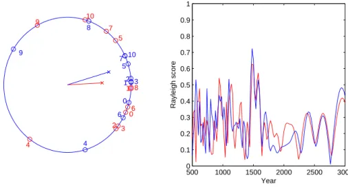
In Fig. 2, right panel, the value ofR(τ) as a function of τ is shown for the two cases NG and G2. The period of 1470 years shows the largest valueR=0.65 (R=0.72 for G2). The angles with respect to the 1470 years period of the time sequence of DO-jumps are plotted on the unit circle in Fig. 2, left panel. The mean phase is indicated

25

by the radial line segments, the length is equal to R(1470 years). The mean phase defines the vertical lines plotted in Fig. 1 (for the NGRIP time scale).

(7)

CPD

2, 1277–1292, 2006

EGU The RayleighR and the Std. dev. res. for the records are listed in Table 1. Omitting

DO9 as proposed by RahmstorfRahmstorf(2003) makes a big difference for the GISP2 dating, but not for the NGRIP dating.

5 Significance of period

The next, and necessary, step in the analysis is to test the significance of the periodicity

5

found in the data. This can only be done by assuming a test-model generating the data. Given such a model, we may choose any measure derived from the data,x_d to compare with the same measure derived from similar realizations of the test-model,xm.

The null-hypothesis is then that the data series is a specific realization of the model. It is important to note that a null hypothesis can only be rejected and not confirmed. That

10

is, the value of the chosen measure for the data may well be within the high likelihood region for the model, but this does not prove that the data cannot be generated from another (competing) model with same high likelihood for the chosen measure. On the contrary, only if the measure for the data falls within a low likelihood region, say with probability-measurep≪1, the model can be rejected with probability 1−p.

15

6 Model 1: Exponential distribution

The simplest possible model which can be chosen for the statistical test is that the DO-events occur randomly, without a memory, on the millennial time scale. This is de-scribed by an exponential distribution for the waiting times corresponding to a Poisson process. The mean waiting time can be assumed to be 2800 years. This is obtained

20

as an estimate from the mean waiting times for 14 DO-events in the period 10–50 kyr. This is also the estimate obtained from the best fit to an exponential distribution of all DO events in the full glacial period (Ditlevsen et al.,2005).

To test the data against this model we use the two measures, the Rayleigh R and the standard deviation of residuals, obtained from the data. For each of the measures

(8)

CPD

2, 1277–1292, 2006

EGU a probability density for a sample, similar to the observed record, is obtained from

a Monte Carlo generated ensemble of 1000 realizations. The results are shown to-gether with the measures from the data records in Fig. 3, top panels. To account for the dating uncertainty an additional uncorrelated gaussian noise, withσ=100 yr corre-sponding to a conservative error estimate, was added to the model signal. In terms

5

of the probability density,p(t)= exp(−t/τ)Φ[(t−σ2/τ)/σ]/τ substitutes the exponential densityp(t)= exp(−t/τ)/τ, where σ is the standard deviation of the dating noise and Φ[x] is the error function. With σ<200 yr this had an insignificant influence on the result and is for simplicity omitted in the following.

From the figure it is obvious that the data records fall within the high likelihood region

10

of the exponential distribution for both measures. The 90% (dashed) and 99% (full) confidence levels are shown in the figure as vertical blue bars. Note that the confidence levels are accurately calculated from the cumulated distribution, independent of the binning used for the histogram. Thus there is no basis for rejecting the hypothesis of no-periodicity for the data. An exception is the curious case of the GISP2 dating with

15

DO9 omitted, in which case the model can be rejected at the 99% confidence level.

7 Model 2: Periodic beating

The opposite proposition of rejecting a periodic component depends on the additional independent noise in the signal. Assuming a perfect periodic beating, with occasional omissions, blurred by the dating noise, the time series model to test data against is

20

t_i=_τ₀+_{n(i)τ, where τ=1470 yr, n(i) is a monotonous integer function and ǫ}_i _{is an} in-dependent unit variance gaussian noise. The standard deviationσ is taken to be 100 years corresponding to the conservative estimate for the dating of the two ice-core records. The results from a simulation of 1000 realizations of this model are shown in Fig. 3, middle panels. This model can be rejected at the 99% confidence level in all 5

25

cases. Now it is highly improbable that a hitherto undiscovered period of such domi-nance should exist in the climate system. The climate system is dominated by internal

(9)

CPD

2, 1277–1292, 2006

EGU noise masking possible periodic components. Thus a more reasonable assumption is

that a periodicity is caused by an internal non-linear amplification of a weak external periodic forcing. This could be described by a stochastic resonance as proposed by Alley et al.(2001).

8 Model 3: Stochastic resonance

5

The stochastic resonance modelBenzi et al.(1982) is defined by the governing equa-tion:

dx= − ∂xUa(x, t, τ)d t+σd B={−2(x3−x)+a cos(2πt/τ)}d t+σd B,

where a particularly simple form of the drift potentialUa(x, t, τ) is chosen here. The

po-tential is a double-well popo-tential, which changes periodically with periodτ from having a

10

shallow well (s) to the right and a deep well (d) to the left to the opposite situation. The ratio of the barrier heightsHs→d/Hd →s is determined by the model parametera. The

time scales for jumping from the shallow well to the deep well is given by an Arrhenius formula; T_s→d∼ exp(Hs→d/2σ

2

), and similarly for T_{d →s}. The criterion for resonance, where the signal x is most periodic, is Ts→d≪τ≪Td →s. This determines the noise

15

intensityσ.

The proposition of rejecting a stochastic resonance (SR) model for the ice-core data is more tricky, since there exists a continuum of SR-models with waiting time distribu-tions from the exponential to the delta-distribution for the perfect periodicity (Ditlevsen et al., 2005). However, the only spectral weight notably above the continuum is at

20

τ−1=1470 years−1 (for the GISP2 dating) and not at the mean waiting time 2800 years−1. Near the stochastic resonance one should expect the same order of mag-nitude “early jumps” (corresponding to a noise induced jump from the deep well to the shallow well) as “late jumps” (corresponding to missing a jump from the shallow to the deep well). The mean waiting time being about twice the observed spectral period

in-25

(10)

CPD

2, 1277–1292, 2006

EGU SR parameters, this means that the criterion; Ts→d≪τ≪Td →s (Ts→d being the mean

waiting time for a transition from the shallow to the deep well), is not fulfilled. We rather seeτ<T_s→d.

Here we test against three SR-models with the period τ=1470 years and a=0.1, 0.2, 0.4. The mean number of DO-events being 11 events/31 kyr corresponding

5

to the climate record. This determines the noise intensity to beσ=0.38, 0.35, 0.27 for the three models.

An ensemble of 1000 simulations with same length as the data records were gener-ated and the same three significance tests were performed. The results for the three models; a=0.1 (light green), a=0.2 (medium green) a=0.4 (dark green) are shown in

10

Fig. 3, panels (e) and (f). The distributions in panels (a) and (b), for the exponential distribution, are overplotted in gray in panels (e) and (f). It is seen that the first model, a=0.1, apparently has less periodicity, represented by Rayleigh’s R, than the purely exponential model. This is because, in the case of the SR model, the distribution is of R(1470 yr), while in the case of the exponential waiting time distribution (corresponding

15

toa=0), the distribution is for the largest value of R found in the sample. (Note that for the Nyquist frequency all points are aligned withR=1. This trivial limit is obviously excluded.) This means that for the SR model witha=0.1, the period will not be identi-fied in comparison to other spurious coincidental periodicities. We have thus identiidenti-fied the “weakest” SR model which may be identified for a sample of the size of the record,

20

and this SR model (a=0.2) is less likely for the data than the exponential waiting time model.

9 Conclusions

In conclusion, the statistical tests show that the waiting times for DO events are within the high likelihood region of the exponential distribution (Figs. 3a, b). This

distribu-25

tion implies that there is no long term memory in the climate system or unknown 1470 years periodic forcing triggering the climate shifts. The assumption of the onsets being

(11)

CPD

2, 1277–1292, 2006

EGU determined by a strictly periodic triggering (not activating at each period) masked by

the dating uncertainty can with high significance be rejected (Figs. 3c, d) A remarkable exception for the rejection is the situation where DO9 is omitted for the GISP2 time scale. The relatively strong periodicity in that case is, however, not preserved in the newer NGRIP dating. By the nature of the statistical test we can only reject the

hypoth-5

esis of a periodic component when the period is sufficiently above the noise level. For SR models with too low a strength of the periodic component, the period would with high probability not be detected in comparison to detecting a spurious coincidental periodicity in the sample (Figs. 3e, f).

References

10

Alley, R. B., Shuman, C. A., Meese, D. A., Gow, A. J., Taylor, K. C., Cuffey, K. M., Fitzpatrick, J. J., Grootes, P. M., Zielinski, G. A., Ram, M., Spinelli, G., and Elder, B.: Visual-stratigraphic dating of the GISP2 ice core: Basis, reproducibility and application, J. Geophys. Res., 102,

26 367–26 381, 1997. 1289

Alley, R. B., Anandakrishnan, S., and Jung, P.: Stochastic resonance in the North Atlantic,

15

Paleoceanography, 16, 190–198, 2001. 1279,1280,1284

Andersen, K. K., Svensson, A., Rasmussen, S. O., Steffensen, J. P., Johnsen, S., Bigler, M., R ¨othlisberger, R., Ruth, U., Siggaard-Andersen, M.-L., Dahl-Jensen, D., Vin-ter, B. M., and Clausen, H. B.: The Greenland Ice Core Chronology 2005, 15–42 ka.

Part 1: Construction of the time scale, QSR Shackleton special edition, in press,

20

doi:10.1016/j.quascirev.2006.08.002, 2006. 1278,1280,1289

Benzi, R., Parisi, G., Sutera, A., and Vulpiani, A.: Stochasic resonance in climate change, Tellus, 34, 10–16, 1982. 1284

Braun, H., Christi, M., Rahmstorf, S., Ganopolski, A., Mangini, A., Kubatski, C., Roth, K., and Kromer, B.: Possible solar origin of the 1,470-year glacial climate cycle demonstrated in a

25

coupled model, Nature, 438, 208–211, 2005.1280

Dansgaard, W., Johnsen, S. J., Clausen, H. B., Dahl-Jensen, D., Gundestrup, N. S., Hammer, C. U., Hvidberg, C. S., Steffensen, J. P., Sveinbjornsdottir, A. E., Jouzel, J., and Bond, G.:

(12)

CPD

2, 1277–1292, 2006

EGU

Evidence for general instability of past climate from a 250-kyr ice-core record, Nature, 364,

218–220, 1993. 1280

Ditlevsen, P. D., Kristensen, M. S., and Andersen, K. K.: The recurrence time of Dansgaard-Oeschger events and limits on the possible periodic component, J. Climate, 18, 2594–2603, 2005. 1278,1280,1281,1282,1284

5

Grootes, P. M. and Stuiver, M.: Oxygen 18/16 variability in Greenland snow and ice with 10−3 -to 105-year time resolution, J. Geophys. Res., 102, 26 455–26 470, 1997. 1278

Huybers, P. and Wunsch, C.: Obliquity pacing of the late Pleistocene glacial terminations,

Nature, 434, 491–494, 2005. 1281

Johnsen, S. J., Dahl-Jensen, D., Gundestrup, N., Steffensen, J. P., Clausen, H. B., Miller, H.,

10

Masson-Delmotte, V., Sveinbjørnsdottir, A. E., and White, J.: Oxygen isotope and palaeotem-perature records from six Greenland ice-core stations: Camp Century, Dye-3, GRIP, GISP2,

Renland and NorthGRIP, J. Quat. Sci., 16, 299–307, 2001. 1278

Meese, D. A., Gow, A. J., Alley, R. B., Zielinski, G. A., Grootes, P. M., Ram, M., Taylor, K. C., Mayewski, P. A., and Bolzan, J. F.: The Greenland Ice Sheet Project 2 depth-age scale:

15

Methods and results, J. Geophys. Res., 102, 26 411–26 423, 1997.1281

Muscheler, R. and Beer, J.: Solar forced Dansgaard/Oeschger events?, Geophys. Res. Lett.,

33, L20706, doi:10.1029/2006GL026779, 2006. 1280

North GRIP members: High resolution Climate Record of the Northern Hemisphere reaching into the last Glacial Interglacial Period, Nature, 431, 147–151, 2004.1278

20

Rahmstorf, S.: Timing of abrupt climate changes: A precise clock, Geophys. Res. Lett., 30,

1510–1514, 2003. 1280,1281,1282

Schulz, M.: On the 1470-year pacing of Dansgaard-Oeschger warm events, Paleoceanography,

17, doi:1029/200PA000571, 2002. 1279,1281

Svensson, A., Andersen, K. K., Bigler, M., Clausen, H. B., Dahl-Jensen, D., Johnsen, S.,

25

Muscheler, R., Rasmussen, S. O., R ¨othlisberger, R., Steffensen, J. P., and Vinter, B. M.: The Greenland Ice Core Chronology 2005, 15–42 ka. Part 2: Comparison to other records, QSR Shackleton special edition, in press, doi:10.1016/j.quascirev.2006.08.003, 2006.1278, 1279,1281

Wunsch, C.: On sharp spectral lines in the climate record and the millennial peak,

Paleo-30

(13)

CPD

2, 1277–1292, 2006

EGU

Table 1. The Rayleigh R and the Std. dev. of residuals for the 5 cases: NG: DO 0–10, NGRIP

timescale, G2: DO 0–10, GISP2 timescale, NG-D09: DO 0,A,1–8,10, NGRIP timescale, G2-D09: DO 0,A,1–8,10–12, GISP2 timescale (Rahmstorf, 2003), DKA-2005: DO1c,1,2a,2b,3–10, NGRIP timescale (Ditlevsen, Kristensen and Andersen,2005). Note that the case G2-D09 is remarkably more periodic than the other 4 cases.

Rayleigh R Std. dev. res.

NG 0.65 0.92

G2 0.72 0.80

NG-D09 0.73 1.01

G2-D09 0.87 0.65

(14)

CPD

2, 1277–1292, 2006

Printer-friendly Version Interactive Discussion EGU ✂ ✂✁☎✄✝✆ ✞ ✄ ✒ ✍

Fig. 1. Theδ18O isotope records from NGRIP and GISP on their stratigraphic time scales (Alley et al.,1997;Andersen et al.,2006). The vertical bars are separated by 1470 years. The analysis focus on the well defined fast onsets of DO events, which are the transitions from the stadial to the interstadial states. Beginning at GIS0 the onset for the DO events are for the NGRIP GICC05 (GISP2) time scale: 11 700 (11 660); 13 130 (13 180); 14 680 (14 700); 23 340 (23 560); 27 780 (27 920); 28 900 (29 100); 32 500 (32 400); 33 740 (33 700); 35 480 (35 360); 38 220 (38 480); 40 160 (40 280); 41 460 (41 240). Ages are b2k=BP+50 years.

(15)

CPD

2, 1277–1292, 2006

Printer-friendly Version Interactive Discussion EGU −1 −0.5 0 0.5 1 0 1 2 3 4 5 6 7 8 9 10 0 12 3 4 5 6 7 8 9 ₁₀ 500 1000 1500 2000 2500 3000 0 0.1 0.2 0.3 0.4 0.5 0.6 0.7 0.8 0.9 1 Year Rayleigh score

Fig. 2. The Rayleigh R test for the two records. The maximum is obtained for the period

τ=1470 years. Left panel shows the timing of the onsets t_n plotted on the unit circle using the transformationθ_n=2πt_n/τ. The red dots represents the NGRIP dating (NG) while the blue

dots represents the GISP2 dating (G2). The segments of radians points at the mean phase, corresponding to the vertical bars in Fig. 1 (for NGRIP dating).

(16)

CPD

2, 1277–1292, 2006

Printer-friendly Version Interactive Discussion EGU 0.4 0.5 0.6 0.7 0.8 0.9 1 0 1 2 3 4 5 6 Max Rayleigh R P ro b a b il it y d e n si ty NG G2 G 2-D O 9 NG -D O 9 D K A -2005 A 0.2 0.4 0.6 0.8 1 1.2 1.4 0 0.5 1 1.5 2 2.5 3 Std. dev. of residuals NG G 2 G 2-D O 9 NG -D O 9 D K A -2005 B 0.4 0.5 0.6 0.7 0.8 0.9 1 0 5 10 15 Max Rayleigh R P ro b a b il it y d e n si ty NG G2 G 2-D O 9 NG -D O 9 D K A -2005 C 0.2 0.4 0.6 0.8 1 1.2 1.4 0 1 2 3 4 Std. dev. of residuals NG G 2 G 2-D O 9 NG -D O 9 D K A -2005 D 0.4 0.5 0.6 0.7 0.8 0.9 1 0 5 10 15 20 Rayleigh R(1470 yr) P ro b a b il it y d e n si ty E 0.2 0.4 0.6 0.8 1 1.2 1.4 0 2 4 6 8

Std. dev. res. (1470 yr)

F

(17)

CPD

2, 1277–1292, 2006

EGU

Fig. 3. Panels (A) and (B): By Monte Carlo an ensemble of 1000 realizations of waiting times

in a 40 kyr period has been generated from an exponential distribution with mean waiting time of 2800 years, corresponding to 14 DO-events in 40 kyr. This gives probability densities for the maximal Rayleigh’s R(τ) in the range 500 yr<τ<5000 yr and for the “Standard deviation

of residual” (see text). The red bars give the values for the ice-core records (see text). The blue bars are 90% (dashed) and 99% (full) confidence levels. Panels (C) and (D): Same as panels (A) and (B), where now the distribution functions are obtained for a perfect 1470 year periodic signal subject to a dating error taken to be a gaussian with standard deviation of 100 years. Panels (E) and (F): Same as panels (A) and (B), with distribution functions obtained from stochastic resonance models with period of 1470 years. From light to dark green the model parameters are: a=0.1, 0.2, 0.4 andσ=0.38, 0.35, 0.27 (see text), which generates on

average 11 DO-events in 31 kyr. The important difference from the case shown in the panels above is that the Rayleigh’s R and Std. dev. of residual in this case are calculated for the fixed period of 1470 yr. The red bars are ice-core data as above. The gray curves are the distributions for the exponential model repeated from the top panels. This shows that the SR model witha=0.1 cannot be identified in a sample, since spurious coincidental periodicities will