Linking glacial and future climates through an ensemble of GCM simulations

(1)

HAL Id: hal-00298153

https://hal.archives-ouvertes.fr/hal-00298153

Submitted on 12 Oct 2006

HAL is a multi-disciplinary open access

archive for the deposit and dissemination of sci-entific research documents, whether they are pub-lished or not. The documents may come from teaching and research institutions in France or abroad, or from public or private research centers.

L’archive ouverte pluridisciplinaire HAL, est destinée au dépôt et à la diffusion de documents scientifiques de niveau recherche, publiés ou non, émanant des établissements d’enseignement et de recherche français ou étrangers, des laboratoires publics ou privés.

Linking glacial and future climates through an ensemble

of GCM simulations

J. C. Hargreaves, A. Abe-Ouchi, J. D. Annan

To cite this version:

J. C. Hargreaves, A. Abe-Ouchi, J. D. Annan. Linking glacial and future climates through an ensemble of GCM simulations. Climate of the Past Discussions, European Geosciences Union (EGU), 2006, 2 (5), pp.951-977. �hal-00298153�

(2)

CPD

2, 951–977, 2006

Linking glacial and future climates J. C. Hargreaves et al. Title Page Abstract Introduction Conclusions References Tables Figures J I J I Back Close

Full Screen / Esc

Printer-friendly Version Interactive Discussion

EGU

Clim. Past Discuss., 2, 951–977, 2006 www.clim-past-discuss.net/2/951/2006/ © Author(s) 2006. This work is licensed under a Creative Commons License.

Climate of the Past Discussions

Climate of the Past Discussions is the access reviewed discussion forum of Climate of the Past

Linking glacial and future climates

through an ensemble of GCM simulations

J. C. Hargreaves1, A. Abe-Ouchi1,2, and J. D. Annan1

1

FRCGC/JAMSTEC, Yokohama, Japan

2

CCSR, Tokyo, Japan

Received: 22 September 2006 – Accepted: 10 October 2006 – Published: 12 October 2006 Correspondence to: J. C. Hargreaves (jules@jamstec.go.jp)

(3)

CPD

2, 951–977, 2006

Full Screen / Esc

EGU

Abstract

In this paper we explore the relationships between the modelled climate of the Last Glacial Maximum (LGM) and that for doubled atmospheric carbon dioxide compared to the pre-industrial climate by analysing the output from an ensemble of runs from the MIROC3.2 GCM.

5

Our results lend support to the idea in other recent work that the Antarctic is a useful place to look for historical data which can be used to validate models used for climate forecasting of future greenhouse gas induced climate changes, at local, regional and global scales. Good results may also be obtainable using tropical temperatures, par-ticularly those over the ocean. While the greater area in the tropics makes them an

10

attractive area for seeking data, polar amplification of temperature changes may mean that the Anatarctic provides a clearer signal relative to the uncertainties in data and model results. Our result for Greenland is not so strong, possibly due to difficulties in accurately modelling the sea ice extent.

The MIROC3.2 model shows an asymmetry in climate sensitivity calculated by

de-15

creasing rather than increasing the greenhouse gases, with 80% of the ensemble hav-ing a weaker coolhav-ing than warmhav-ing. This asymmetry, if confirmed by other studies would mean that direct estimates of climate sensitivity from the LGM are likely to be underestimated by the order of half a degree. Our suspicion is, however, that this re-sult may be highly model dependent. Analysis of the parameters varied in the model

20

suggest the asymmetrical response may be linked to the ice in the clouds, which is therefore indicated as an important area for future research.

1 Introduction

Paleoclimate simulations provide an opportunity to validate model performance under substantially different conditions to the modern climate. Nevertheless, most effort in

cli-25

(4)

CPD

2, 951–977, 2006

Full Screen / Esc

EGU

the present day climate. However, recent work (Annan et al.,2005) has shown that this is by no means a guarantee of success: it is possible to improve the representation of the present day (quasi steady-state) climate in a model while simultaneously decreas-ing the accuracy of its representation of climate change in response to substantial historical changes in boundary conditions (and therefore presumably worsening

pre-5

dictions of future change). Therefore, it is important to consider whether there are other ways of gaining confidence in, and improving the accuracy of, model predictions. The last glacial maximum (LGM) epoch has long been recognised as a time which might provide useful information for inferring future climate changes (e.g.Manabe and

Brocolli, 1985), due to the fact that it is the most recent time (and therefore the time

10

for which paleoclimate data is available in some quantity and quality) when forcings, (including those from greenhouse gases), and the climate state itself, were significantly different from the modern era. Since the net forcing at that time was strongly negative, and includes large contributions from factors other than greenhouse gas levels (most notably, large ice sheets in the northern hemisphere), it is unclear as to how directly we

15

can infer future climate changes based on the LGM state. Nevertheless, there is still useful evidence here, especially when considered in combination with other lines of evidence which are individually somewhat weak but collectively rather more convincing (Annan and Hargreaves,2006). Furthermore, even if paleoclimate simulations provide only limited validation of climate predictions, not undertaking such studies at all could

20

hardly be argued to be a better strategy.

Annan et al.(2005) found a correlation between modelled LGM (global and tropical) 2 m temperature (T2) change and global T2 change (compared to the modern climate) for doubled atmospheric carbon dioxide (2×CO2) in the MIROC3.2 GCM (Hasumi and

Emori, 2004). In that work the data used to validate the model’s LGM state were

25

the PMIP1 Alkenone data (http://www-lsce.cea.fr/pmip/,Harrison,2000) from from the tropical ocean region. These data have been widely used (e.g.IPCC,2001, Chapter 8) and provide coverage over a substantial proportion of the Earth’s surface, so were therefore assumed to be reasonably representative of global climate change, but this

(5)

CPD

2, 951–977, 2006

Full Screen / Esc

EGU

question is still very much open. The availability and precision of regionally inhomoge-neous data, the understanding of the forcings that dominate over particular geographi-cal areas, and the confidence with which past and future changes can be linked are all factors which may affect which data are most useful for validating and improving model performance.

5

A recent examination of a multi-model ensemble from a range of different ex-periments (broadly PMIP1, PMIP2 and CMIP; http://www-lsce.cea.fr/pmip/, http:

//www-lsce.cea.fr/pmip2/ and http://www-pcmdi.llnl.gov/projects/cmip/index.php, re-spectively) was undertaken byMasson-Delmotte et al.(2006) (hereafter MD06), with the focus of assessing the potential value of polar ice cores for providing “quantitative

10

insights on global climate change”. Although their results were somewhat inhibited by small sample statistics, they concluded that there was a clear correlation between the global average and polar temperature changes compared to the control climates in the models for both the LGM and increased CO2 experiments. However, due to very limited overlap between the model populations which were integrated for LGM, and

15

increased CO2 states, they did not in fact analyse whether whether the polar or global LGM temperature changes were related, in the models, to the global or polar temper-ature changes for the increased CO2 states, although they considered their results to be consistent with the hypothesis that such a relationship does exist. Crucifix(2006) investigated this question with the set of 4 models for which both LGM and doubled

20

CO2 integrations are available, and found no evidence of a relationship between global or tropical temperature changes. With only 4 coupled atmosphere-ocean model runs available which covered a modest range of climate sensitivity, it is not yet clear to what extent LGM simulations can help to narrow the rather wider range of model results that has sometimes been presented as plausible (e.g.Andronova and Schlesinger,2001;

25

Stainforth et al., 2005). von Deimling et al. (2006) found a strong relationship be-tween LGM and 2×CO2 conditions across an ensemble of a simple climate model with uncertain parameters allowed to vary, butAnnan et al. (2005) found a rather weaker relationship with a more sophisticated model which has more sources of uncertainty.

(6)

CPD

2, 951–977, 2006

Full Screen / Esc

EGU

In this paper we extend our previous analysis and consider further the conclusions presented by MD06, by considering a large perturbed-parameter ensemble from one particular model (MIROC3.2Hasumi and Emori,2004). While we are able to integrate numerous pairs of identical model versions for both LGM and 2×CO2 climates and therefore do not have such a severe problem with small sample statistics, our results

5

are necessarily tentative because we show results from only one model, and as MD06 showed, results can vary considerably between different models. In addition, for com-putational reasons we are using the model in a slab ocean configuration, rather than the fully coupled model which is now state-of-the-art for PMIP2. However, our results suggest areas where further investigations may be worthwhile with a wider range of

10

models. Also, where even a single-model ensemble generates negative or weak re-sults, it seems unlikely that a multimodel ensemble, which introduces more sources of uncertainty, will generate anything more useful.

We broaden the scope of the MD06 work, by considering not only annual average temperatures at the poles, but consider more broadly the zonal variation, the effects

15

of land and ocean and also the seasonal variations. The main motivation for this is that data are available at a wide range of latitudes, and some are plausibly consid-ered more directly representative of seasonal changes (e.g. precipitation-dependent proxies) rather than annual averages.

In order to further explore the value of the LGM climate for estimating climate

sensi-20

tivity we also compare the results from an experiment where we do not impose massive ice sheets or the insolation forcing of the LGM state, and thus the only change com-pared to the control run is that the levels of greenhouse gases (GHG) are changed to the LGM levels prescribed by PMIP2.

In Sect.2 we outline the way the ensemble of model runs was formed and discuss

25

the climate states that were modelled. In Sect. 3 we discuss the results focussing principally on a zonal analysis of the T2 temperature changes. In Sect.4we discuss the implications of our results for the calculation of climate sensitivity. In Sect.5we briefly touch on the complex issue of attributing the climate changes to variation in individual

(7)

CPD

2, 951–977, 2006

Full Screen / Esc

EGU

parameters, and then we conclude with an overview of the results and discussion of the wider implications.

2 Methods

2.1 Ensemble of MIROC3.2 runs

For these experiments we use the T21L20 slab-ocean version of the state-of-the

5

art GCM MIROC3.2 (Hasumi and Emori, 2004). The atmospheric component is a reduced-resolution version of the standard T42 version used in several modelling stud-ies, including the results analysed by MD06 and Crucifix (2006). The physical and numerical schemes are unchanged, and a “control run” (with the parameter values taken directly from the control T42 model, with the exception of the strongly

resolution-10

dependent gravity wave drag parameter) produced similar results to those of the higher resolution model at both LGM and 2×CO2 states. We used the ensemble Kalman filter (EnKF) to generate three ensembles each of 40 members (Annan et al.,2005). For each experiment, we used the same expert opinion for the prior ranges of 25 parame-ters which we allowed to vary. The model was tuned to seasonally-averaged (summer

15

and winter only) fields of 15 different climatological variables such as temperature, pre-cipitation, radiation and winds. The only difference between the three experiments was in the judgment as to the model error that we considered reasonable. One ensemble consists of models which actually reproduce the climate fields better (as indicted by a normalised RMS error measure) than the control run, and the other two were less

20

tightly tuned to the data and so covered a wider range of the parameter space. The experiment is described more fully inAnnan et al.(2005). Taken as a whole we have a set of runs which all compare reasonably well with present day climatology but with dif-ferent values for all the 25 varied parameters. A general understanding of model error is at present rather limited, and the model results exhibit a bias towards high sensitivity

25

(8)

(fur-CPD

2, 951–977, 2006

Full Screen / Esc

EGU

ther investigations and development of the model is ongoing) so we simply combine the three ensembles in our analysis to explore the emergent relationships between different climate states that appear significant in the context of our experiment.

2.2 Model runs

After the parameter sets were generated, we then performed 4 experiments with all

5

the model instances: pre-industrial (CTRL) climate, doubled CO2 (2×CO2), LGM (with PMIP2 boundary conditions) and LGMGHG (greenhouse gases and orbital parameters as for PMIP2, but without the ice sheet and insolation changes of the PMIP2 protocol). Table1gives an overview of the forcings for the 4 experimental model climates. The experiments were run until the annual average temperatures had converged (at least

10

24 years for LGM and LGMGHG, 36 years for 2×CO2) and then a further 20 years were averaged for the climatological results discussed below.

The 120 member ensemble was run for each of the 4 experiments, but only 119 runs were used in the analysis. One model run, under LGMGHG boundary conditions, ex-hibited runaway cooling with no sign of equilibrating over a 50 year integration. Strong

15

cooling was centred on the eastern equatorial Pacific. This behaviour appears to be due to the same phenomenon as that noted byStainforth et al.(2005) (a non-physical localised cooling instability arising from the limitations of a slab ocean model), and we therefore exclude this member from all of our analyses. Since we are seeking to analyse the relevance of paleo-temperature data for future temperature change

pre-20

diction, we confine our analysis here to consideration of the modelled surface (2 m) temperatures.

We have analysed the 119 member ensemble to look at the correlations between several different components of both model variables, and also the relationship of these with the parameters. The correlations indicate the extent to which our uncertainties

25

about the climate system (as encapsulated by imperfectly known parameter values in the model equations) affect past and future climate simulations in similar ways. Where the historical simulation is weakly related to the future, then increasing our skill in this

(9)

CPD

2, 951–977, 2006

Full Screen / Esc

EGU

aspect of the simulation will hardly affect our predictions, even if it does increase our understanding of some physical processes. Conversely, a strong relationship would suggest that simulations which were quantitatively improved in this area could reason-ably be expected to give a more accurate and reliable forecast.

For 119 independent samples from a distribution, the 99% significant correlation

co-5

efficient from the student T test is 0.24. Our ensemble is a somewhat ad-hoc mixture of three 40 member ensembles, so, in the rather qualitative discussion in this paper, we use this value as a guide as to the strength of the correlation rather than a definitive threshold. It is also possible that a different experiment with MIROC3.2, varying differ-ent parameters and making different prior assumptions could produce an ensemble of

10

similarly reasonable model runs with rather different resultant characteristics. Due to the substantial investment in time required to perform this experiment (several months), we have not yet undertaken a repeat experiment of this nature, although one is planned for the future which will also use a revised and updated version of the model. In the following discussion we consider a correlation above 0.5 to be strong and one below

15

0.3 to be weak. Since our model has a relatively low-resolution T21 grid, we do not expect accurate results at the grid-point level for comparison with in-situ data. There-fore, we focus on zonal averages rather than the location-based estimates. However, for comparison with the MD06 results we have also derived some results for Greenland and Antarctica. It should also be noted that it was recently discovered that this version

20

of the model contained a bug which generated a bias in the air temperatures over land ice. However it does not seem likely that this will have affected our analysis which focusses on the correlations between temperature changes, rather than the absolute values themselves.

3 Correlation between LGM and doubled CO2 temperature changes

25

The ensemble mean, annually averaged T2 results are shown in Fig.1, with subplot A showing the CTRL results and the other three subplots showing the differences in

(10)

tem-CPD

2, 951–977, 2006

Full Screen / Esc

EGU

perature between the each specific climate state and the CTRL. The zonal temperature changes for December, January and February (DJF) and June, July and August (JJA) for the three experiments and also the actual average temperatures for the control run are illustrated in Fig.2. The existence of a strong “polar amplification” (as discussed by MD06) of the temperature changes can be seen in the results from this model.

5

Crucifix (2006) quotes the following observational estimates of climate change: Antarctica, –9±2◦C (Jouzel et al.,2003); Greenland, −20±2◦C (Cuffey and Clow,1997;

Dahl-Jensen et al.,1998); and the tropical ocean, −2.7±0.5◦C (Ballantyne et al.,2005;

Lea,2005). For comparison with these results we have the following mean and 1 stan-dard deviation range for our ensemble: Antarctica, −9±1.3◦C; Greenland, −18±2◦C;

10

tropical ocean, −3.0±0.5◦C. Here we quote the average 2m temperatures over the Greenland and Antarctic land masses and the tropical region includes the ocean grid boxes between latitudes 30◦S and 30◦N. We note that the PMIP2 boundary conditions excluded some forcings (vegetation and dust) which are thought to be significant and negative, which supports our belief that our ensemble of models has an overall bias

15

towards high sensitivity.

3.1 Global and tropical analysis

Figure 3 shows scatter plots for the globally averaged T2 changes for both LGM and LGMGHG verses 2×CO2, illustrating the smaller T2 changes (as expected) for LGMGHG. The correlation between the T2 changes is clear. The correlation coe

ffi-20

cients for these results and some others are given in Table2. The correlation coefficient is stronger between 2×CO2 and LGM climates when looking at the tropics only. The LGMGHG global T2 change is more highly correlated with LGM than 2×CO2 climates. This is perhaps surprising since, if the response to changes in greenhouse gas forcing was linear across the range covered by the 2×CO2 and LGMGHG states, then one

25

would expect the correlation between these two states to be the stronger, because the LGM climate state is also strongly influenced by the large ice sheet and to a lesser extent by changes in solar forcing. It seems, therefore, that a large proportion of

(11)

un-CPD

2, 951–977, 2006

Full Screen / Esc

EGU

certainty in the model response is due to a nonlinearity in the response to positive and negative forcings, which we discuss further in Sect.4.

3.2 Zonal analysis

Here we consider how the globally and zonally averaged patterns of temperature change are correlated for the different experiments.

5

3.2.1 Doubled CO2 experiment

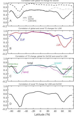
The dashed line in Subplot A of Fig.4shows that, unsurprisingly, the correlation be-tween the temperature changes for global and zonally averaged temperature change for the 2×CO2 climate is strong at all latitudes, although there is a notable drop in the southern sea-ice region (around 65◦S). Small changes in sea ice extent cause large

10

localised temperature changes due to the positive feedback of the albedo effect. Even with ocean heat fluxes calculated to reasonably reproduce the present day climate, the ensemble members have somewhat different sea-ice extents in the modern climate, which results in substantially different temperature changes in this region when the ice extent shrinks (vanishes) in the warmer climate. Thus, the temperature change is

15

strongly influenced by small biases in the initial sea ice extent. 3.2.2 LGM experiment

There is also also generally a high correlation between the global and zonally averaged temperature change at the LGM. Figure4subplot B shows this result split into DJF and JJA seasons. Both polar sea-ice regions (but not the poles themselves) show markedly

20

lower correlation in the summer seasons, falling away to nothing during JJA for northern high latitudes, where the northern hemisphere ice sheets and sea ice are located.

With a lack of identical models run for both 2×CO2 and LGM conditions, the rela-tionship between the two was assumed by MD06. Here we examine the relarela-tionship between the LGM and climate sensitivity by looking at the correlation between the

(12)

CPD

2, 951–977, 2006

Full Screen / Esc

EGU

magnitudes of the zonally averaged LGM and globally averaged 2×CO2 temperature changes. This result is shown as the solid black lines in subplots A and C of Fig. 4. While still high in places (including Antarctica), it is considerably lower (especially at northern latitudes) than the correlation between global and zonally averaged LGM tem-perature change. Areas of strong correlation include both central Antarctica and the

5

tropics. The other two lines in subplot C of Fig.4shows the annually averaged results for the same correlation, split into land (magenta) and ocean (cyan). This shows a generally better correlation with the temperature over the ocean than the land between the latitudes of 50◦S and 50◦N. Also shown are the values of the correlation coe ffi-cients for the averages over the Antarctica and Greenland land areas. These show

10

that while the MD06 conclusions are supported with a high correlation for Antarctica, in MIROC3.2 there is not such a high correlation for Greenland. The MD06 results were for central Greenland (>1300 m) and central Antarctica (>2500 m). Although there are differences (<2◦C) in the magnitude of the temperature change, there is not a signifi-cant difference in the correlation coefficients evaluated using the central values rather

15

than the averages. Due to the coarse resolution of our model we show the average land mass values since these are more likely to be robust.

Our results suggest that the tropics, particularly the ocean regions, may also be good places for calibrating and improving models which are then to be used for prediction of future climate change caused by increased greenhouse gas levels. The existence of

20

this particular correlation in the same model has already been used in previous work (Annan et al.,2005), where we attempted to constrain estimates of climate sensitivity using tropical SST data from the LGM. Our results here show that including Antarctic temperature estimates from ice cores into the calculation could potentially improve the result from such an experiment. Despite the small area at the poles, the data there

25

may be less noisy than at the tropics due to the fact that the total temperature changes (Figs.1 and 2) are much greater for the polar regions than the tropics in the winter months (and for the annual mean) for both 2×CO2 and the LGM. Correlations in the sea ice regions and over zones where the Northern ice sheets are situated at the LGM

(13)

CPD

2, 951–977, 2006

Full Screen / Esc

EGU

are weak, suggesting that, at least in our model, these regions are less informative of future climate changes.

Understanding and predicting climate change at smaller scales than global is ob-viously desirable. In this context we would like to know to what extent LGM climate changes can be used to validate the predictive models at the regional scale. As a

5

step towards this we have calculated the correlation between the magnitude of the zonally averaged temperature changes for LGM and 2×CO2 climates. The resulting variation of the correlation coefficient with latitude is similar in shape to that obtained from analysing the globally averaged 2×CO2 and zonally averaged LGM changes. The correlation in the tropical regions is stronger, while insignificant in the southern sea-ice

10

region. This strengthening in those areas that were strongly correlated with global changes might be expected, while the weakening in the sea-ice region indicates that, further to the discussion in Sect.3.2.1, the large non-linear albedo feedback is such that the small differences in the modelled extent of sea ice leads to large differences in the local temperature response to forcing changes.

15

4 Implications for climate sensitivity

Correlation coefficients for the LGMGHG experiment, where only the greenhouse gases were changed to LGM levels but all other forcings were kept the same as the control run, are shown in Table 2. As already discussed in Sect. 3.1 the LGMGHG temperature changes are more strongly correlated with the LGM temperature changes

20

than the 2×CO2 temperature changes. As is apparent from Fig.3 there is almost as much scatter in the LGMGHG vs 2×CO2 (red) temperatures as there is for the LGM vs 2×CO2 temperatures (blue). This is a somewhat surprising result which implies that the uncertainty in the response to the ice sheet does not outweigh that due only to the nonlinearity in the response to increasing versus decreasing GHG levels.

Look-25

ing at the dot-dashed line in Subplot A of Fig.4which shows the correlation between the magnitudes of the global temperature change for 2×CO2 and zonal temperature

(14)

CPD

2, 951–977, 2006

Full Screen / Esc

EGU

change for LGMGHG, the line more closely follows the LGM zonal variation except north of about 30◦N where the correlation is more like the 2×CO2 zonal variation. So, while the north of the northern hemisphere is largely influenced by the ice sheets at the LGM, it seems that uncertainty in the influence of the ice sheet does not have a clear influence on the rest of the globe and therefore it must be nonlinearity of the

re-5

sponse to differing GHG levels across the range tested that produces a large part of the observed scatter in the relationship between LGM and 2×CO2 climates.

The radiative forcing due to greenhouse gas levels at the LGM is equivalent to –2.8 Wm−2, whereas that caused by doubling CO2 is +3.7 Wm−2. Therefore, if the effects of increasing and decreasing the forcing were equivalent in the model, the

mag-10

nitude of the LGMGHG global temperature changes should be 76% of that for 2×CO2. In Fig.5 we show the histogram of the global temperature changes plotted as a ratio T2(CTRL-LGMGHG)/T2(2×CO2-CTRL). Also shown, with a red line, is the 0.76 value corresponding to equal sensitivity. The line on Fig.3also shows the expected results for the LGMGHG and CO2 experiments if the response to increased and decreased

15

GHG concentrations were linear.

For the median of the ensemble, the difference between the value of climate sen-sitivity and T2(CTRL-LGMGHG)/0.76 is 0.62◦C. Furthermore, close to 80% of the en-semble have a smaller magnitude of temperature change when greenhouse gases are decreased rather than increased. It is easy to imagine that different climate models

20

may show widely varying results in this aspect, given the large differences in their cloud parameterisation schemes. In fact, we have reason to suspect (for reasons discussed below) that the response of MIROC may be somewhat anomalous in this respect, but this conclusion will remain rather tentative until others undertake similar investigations.

5 Correlations between parameter values and temperature changes

25

An in depth discussion of the physical effects of all of the 25 parameters which varied in the EnKF experiments is beyond the scope of this paper (and perhaps of little interest

(15)

CPD

2, 951–977, 2006

Full Screen / Esc

EGU

to those using different models). Here we briefly describe the statistical behaviour of the most significant parameters along with their characteristics to the extent that they illustrate some the results described above.

Table4 shows the correlations of the temperature differences between the experi-mental climate states and the control climate for 9 of the 25 parameters which were

5

allowed to vary independently in the EnKF experiments. These 9 parameters (defined in Table3) are the only ones which individually showed even a marginally (at the pre-viously mentioned 1% level) significant correlation for any of the three experimental climates (considering T2 changes with respect to the CTRL climate) at the global or tropical scale.

10

At the global and tropical scale for the 2×CO2 climate, the clearly dominant pa-rameter is “prctau”, but interestingly, this papa-rameter is less dominant for the LGM and LGMGHG climate states. This parameter is one which directly controls the behaviour of ice in clouds and it seems plausible that the asymmetrical effect between warming and cooling is linked to the distribution of ice in clouds. The relationship of ice, clouds

15

and sensitivity is complex, butTsushima et al.(2006) find less cloud ice to be linked to in a larger poleward shift in cloud water and therefore a reduced cloud albedo effect, amplifying the overall warming. However, at least for the two versions of MIROC con-sidered in that work (among other GCMs) and an intermediate unpublished version, their overall sensitivity to LGM boundary conditions is rather similar, indicating that this

20

change in model formulation has little effect under strong cooling conditions. It remains to be seen whether this effect is robust across models with a wider range of structural differences. If the drier climate at the LGM resulted in a decreased water vapour feed-back then the temperature change for the LGM may vary less between different models than the temperature change for 2×CO2.

25

The other 3 parameters which are significant for the 2×CO2 temperature changes in the tropics are not very significant on the global scale. Zonal analysis (not shown) shows that this is caused by a sharp decrease in the correlation (or even opposite correlation in some cases) in the southern sea ice region. While the LGM temperature

(16)

CPD

2, 951–977, 2006

Full Screen / Esc

EGU

changes also show significant correlation with these parameters particularly in the trop-ics, the LGM picture is further complicated by effects from four other parameters. This result is consistent with the results in Table 2 and Fig. 3, which shows considerable scatter in the relationship between LGM and 2×CO2 temperature changes. Of these 4 additional parameters, 2 (alp, snfrs) are not significant for LGMGHG. It is perhaps

un-5

surprising that alp (gravity wave drag) and snfrs (related to albedo) are more strongly related to the temperature changes over the ice sheet. The overall similarity in the pa-rameters that are significant for both LGMGHG and LGM climate changes is consistent with the general similarity of the results for these two climates shown in Subplot A of Fig.4.

10

6 Conclusions

The model results presented in this paper show that in the MIROC3.2 model there is a reasonably strong link between global and tropical temperature changes at the LGM and those for 2×CO2. However, there is a considerable amount of noise in the correlation, even though we are only considering the results from one model. It is

15

clear that different processes (controlled by different parameters) affect the response to strong positive and negative forcings, even when this forcing is limited to radiative forcing of greenhouse gases. The albedo and topographical influences of large ice sheets complicate matters further, at least at the local level. Unsurprisingly, the links between regional and global scales within the same experimental epoch are much

20

stronger. With a lack of model runs from both climate states, MD06 assumed the link existed, whileCrucifix (2006) obtained results from only 4 simultaneous models and perceived no such link at the global scale. While a perturbed-parameter ensemble can form a step towards increasing our understanding, it is unlikely to cover the full range of results that structurally different models can achieve. It is therefore important, if this

25

link is to be better understood, that directly comparable integrations of both LGM and 2×CO2 climates are performed for a larger number of GCMs in future. Furthermore, it

(17)

CPD

2, 951–977, 2006

Full Screen / Esc

EGU

would be helpful to ensure that the LGM boundary conditions actually represent reality as faithfully as possible, rather than representing a sensitivity analysis in which some potentially important (albeit poorly understood) elements are omitted. This is especially important if a direct comparison with data is to be attempted.

Our results lend support to the idea in MD06 that the LGM Antarctic is a good place

5

to look for a data which can be used to validate models used for climate forecasting of future GHG induced climate changes, at local, regional and global scales. Good results may in principle be obtainable using tropical temperatures, particularly those over the ocean. While the greater area in the tropics makes them an attractive area for seeking data, polar amplification of temperature changes (apparent in Fig.2) may

10

mean that the Anatarctic provides a clearer signal relative to the uncertainties in data and model results. Our result for Greenland is not so strong, possibly due to difficulties in accurately modelling the sea ice extent.

The areas occupied by the massive northern hemisphere ice sheets and sea ice at the LGM would appear to be very poor places to seek data of relevance to GHG

15

forcing. Our results indicate that the temperature changes in those regions are con-trolled by different parameters for both LGM and for the southern sea ice region for the 2×CO2 climate. This implies different processes at work in those regions which there-fore means that changes observed at the present day in the southern sea ice locations would provide only relatively weak information on the value of future globally averaged

20

warming.

The MIROC3.2 model shows an asymmetry in climate sensitivity calculated by de-creasing rather than inde-creasing the greenhouse gases, with 80% of the ensemble hav-ing a weaker coolhav-ing than warmhav-ing. This asymmetry, if confirmed by other studies, would mean that direct estimates of climate sensitivity from the LGM are likely to be

25

underestimated by the order of half a degree. Our suspicion is, however, that this re-sult may be highly model dependent. Analysis of the parameters varied in the model suggest the asymmetrical response may be linked to the ice in the clouds, which is therefore indicated as an important area for future research.

(18)

CPD

2, 951–977, 2006

Full Screen / Esc

EGU

Acknowledgements. We thank the K-1 Japan project members for support and discussion.

This work was partially supported by the Research Revolution 2002 (RR2002) of the Ministry of Education, Sports, Culture, Science and Technology of Japan. The model calculations were made on the Earth Simulator of JAMSTEC.

References

5

Andronova, N. G. and Schlesinger, M. E.: Objective estimation of the probability density func-tion for climate sensitivity, J. Geophys. Res., 108, 22 605–22 611, 2001. 954

Annan, J. D. and Hargreaves, J. C.: Using multiple observationally-based constraints to es-timate climate sensitivity, Geophys. Res. Lett., 33, L06704, doi:10.1029/2005GL025259, 2006. 953

10

Annan, J. D., Hargreaves, J. C., Ohgaito, R., Abe-Ouchi, A., and Emori, S.: Efficiently con-straining climate sensitivity with paleoclimate simulations, SOLA, 1, 181–184, 2005. 953,

954,956,961

Ballantyne, A. P., Lavine, M., Crowley, T. J., Liu, J., and Baker, P. B.: Meta-analysis of tropical surface temperatures during the Last Glacial Maximum, Geophys. Res. Lett., 32, 2005. 959

15

Crucifix, M.: Does the Last Glacial Maximum constrain climate sensitivity, Geophys. Res. Lett., in press, 2006. 954,956,959,965

Cuffey, K. M. and Clow, G. D.: Temperature, accumulation, and elevation in central Greenland through the last deglacial transition, Geophys. Res. Lett., 102, 26 383–26 396, 1997. 959

Dahl-Jensen, D., Modegaard, Gundestrup, N., Clow, G. D., Johnsen, S. J., Hansen, W., and

20

Balling, N.: Past temperatures directly from the Greenland ice sheet, Science, 282, 268–271, 1998. 959

Harrison, S. P.: Palaeoenvironmental data sets and model evaluation in PMIP, in: Proceedings of the third PMIP workshop. WCRP-111; WMO/TD-No. 1007, edited by: Braconnot, P., 9–25, La Huardire, Canada, 2000. 953

25

Hasumi, H. and Emori, S.: K-1 coupled model (MIROC) description, K-1 technical report 1, Tech. rep., Center for Climate System Research, University of Tokyo, 2004. 953,955,956

IPCC: Climate change 2001: the scientific basis. Contribution of Working Group 1 to the Third Assessment Report of the Intergovernmental Panel on Climate Change, Cambridge Univer-sity Press, 2001. 953

(19)

CPD

2, 951–977, 2006

Full Screen / Esc

EGU

Jouzel, J., Vimeux, F., Caillon, N., Delaygue, G., Hoffman, G., Masson-Delmotte, V., and Par-renin, F.: Magnitude of isotope/temperature scaling for interpretation of central Antarctic ice cores, J. Geophys.l Res., 108(D120), 4361, 2003. 959

Lea, D. W.: The 100,000-yr cycle in tropical SST, greenhouse forcing, and climate sensitivity, J. Climate, 17, 2170–2179, 2005. 959

5

Manabe, S. and Brocolli, A. J.: A comparison of climate model sensitivity with data from the last glacial maximum, J. Atmos. Sci., 42, 2643–2651, 1985. 953

Masson-Delmotte, V., Kageyama, M., Charbit, P. B. S., Krinner, G., Ritz, C., Jouzel, E. G. J., Abe-Ouchi, A., Gladstone, M. C. R. M., Hewitt, C. D., LeGrande, A. K. A. N., Marti, O., Merkel, U., Ohgaito, T. M. R., Otto-Bliesner, B., Ross, W. R. P. I., Valdes, P. J., Vettoretti, G.,

10

Wolk, S. L. W. F., and YU, Y.: Past and future polar amplification of climate change: climate model intercomparisons and ice-core constraints, Climate Dyn., 513–529, 2006. 954

Peltier, W.: Global glacial isostasy and the surface of the ice-age Earth: the ICE-5G (VM2) model and GRACE, Ann. Rev. Earth Planet. Sci., 32, 111–149, 2004. 969

Stainforth, D. A., Aina, T., Christensen, C., Collins, M., Faull, N., Frame, D. J., Kettleborough,

15

J. A., Knight, S., Martin, A., Murphy, J. M., Piani, C., Sexton, D., Smith, L. A., Spicer, R. A., Thorpe, A. J., and Allen, M. R.: Uncertainty in predictions of the climate response to rising levels of greenhouse gases, Nature, 433, 403–406, 2005. 954,957

Tsushima, Y., Emori, S., Ogura, T., Kimoto, M., Webb, M. J., Williams, K. D., Ringer, M. A., Soden, B. J., Li, B., and Andronova, N.: Importance of the mixed-phase cloud distribution

20

in the control climate for assessing the response of clouds to carbon dioxide increase: a multi-model study, Climate Dyn., 27, 113–126, 2006. 964

von Deimling, T. S., Held, H., Ganopolski, A., and Rahmstorf, S.: Climate sensitivity estimated from ensemble simulations of glacial climate, Climate Dyn., 27, 149–163, 2006. 954

(20)

CPD

2, 951–977, 2006

Full Screen / Esc

EGU

Table 1. Overview of the forcings imposed for the 4 experimental climates. The forcings labelled

“PMIP2” refer to the forcings for the PMIP2 21kyr experiment, for which the ice sheet is ICE5G V1.1 (Peltier,2004).

run GHG insolation ice sheet CO2 N2O CH4

(ppm) (ppb) (ppb)

CTRL 285 280 860 CMIP CMIP 2×CO2 570 280 860 CMIP CMIP LGM 185 200 350 PMIP2 PMIP2 LGMGHG 185 200 350 CMIP CMIP

(21)

CPD

2, 951–977, 2006

Full Screen / Esc

EGU

Table 2. Correlation coefficients for the magnitude of tropical and global T2 temperature

changes with respect to the CTRL state for the three climates. Only the correlations men-tioned in the text are shown. “gl.” denotes globally averaged T2 changes, and “tr.” denotes averages from the tropical region (30◦S–30◦N).

2×CO2 LGM LGMGHG tr. gl. tr. gl. tr. 2×CO2 gl. 0.94 –0.59 –0.64 –0.67 –0.63 2×CO2 tr. –0.69

(22)

CPD

2, 951–977, 2006

Full Screen / Esc

EGU

Table 3. Parameter definitions for 9 parameters which showed some evidence of significant

correlation with T2 changes at global or tropical scales. parameter description

prctau e-folding time for ice precipitation (m3/kg/s)

elamin min. entrainments factor for cumulus convection (1/m) tefold e-folding time for horizontal diffusion (day)

rhmcrt Critical rel. hum for cum. conv. (–) vice0 ice fall speed factor (m/s)

dffmin min. vert. diff coief (m2/s) alp gravity wave drag factor (rad/m)

snrfrs snow amount required for refreshing snow albedo (kg/m2) ray0 Rayleigh friction e-folding time (day)

(23)

CPD

2, 951–977, 2006

Full Screen / Esc

EGU

Table 4. Correlations of parameters with global and tropical annual average T2 change for

three climate compared to present day. 1% significance for correlations with 119 samples is 0.24. Those correlations greater than this value are marked in bold. See Table3for parameter definitions.

parameter 2×CO2 LGM LGMGHG Global Trop. Global Trop. Global Trop. prctau 0.53 0.51 –0.21 –0.30 –0.33 –0.35 elamin –0.20 –0.39 0.31 0.39 0.35 0.40 tefold 0.19 0.30 –0.26 –0.29 –0.29 –0.22 rhmcrt 0.20 0.24 –0.17 –0.29 –0.25 –0.29 vice0 –0.17 –0.21 0.38 0.32 0.39 0.30 dffmin 0.07 –0.06 0.30 0.30 0.39 0.40 alp –0.21 –0.12 0.33 0.33 0.18 0.13 snrfrs –0.07 –0.11 0.31 0.20 0.19 0.11 ray0 0.19 0.13 –0.19 –0.22 –0.22 –0.25

(24)

CPD

2, 951–977, 2006

Full Screen / Esc

EGU

Fig. 1. Annually averaged T2 temperature: mean of the 119 MIROC3.2 ensemble members. (a): Control (CTRL) run, (b): (2×CO2-CTRL), (c): (LGM-CTRL), (d): (LGMGHG-CTRL).

(25)

CPD

2, 951–977, 2006

Full Screen / Esc

EGU

Latitude (o_N)

T2 (K) CTRL run

T2 (K), (exp. run - CTRL run)

DJF JJA 2xCO2 LGM-GHG LGM LGM LGM-GHG 2xCO2 A C D B

Fig. 2. Top plots: Seasonally averaged (left DJF; right JJA) zonal T2 profiles for the

con-trol (CTRL) climate. Lower plots: Dashed line, (2×CO2-CTRL); solid line, (LGM-CTRL); dot-dashed line, (LGMGHG-CTRL). The lines show the mean and one standard deviations of the 119 member ensemble results.

(26)

CPD

2, 951–977, 2006

Full Screen / Esc

Printer-friendly Version Interactive Discussion EGU T2 change (K) (2xCO2 - CTRL) T2 change (K) (CTRL - LGMGHG) (CTRL - LGM)

Fig. 3. Scatter plot of the magnitude of global annually averaged temperature change (all

changes are magnitudes relative to CTRL state) for 2×CO2 vs. LGM (blue), 2×CO2 vs LGMGHG (red), for the 119 member model ensemble. The red line shows the expected re-sults for the LGMGHG and CO2 experiments if the response to increased and decreased GHG concentrations were linear.

(27)

CPD

2, 951–977, 2006

Full Screen / Esc

Printer-friendly Version Interactive Discussion EGU A B C D Latitude (o_N) Correlation Coeﬃcient DJF JJA land ocean total Antarctica Greenland LGM 2xCO2 LGM-GHG

Correlation of global and zonal T2 changes for LGM

Correlation of T2 change, global for 2xCO2 and zonal for LGM

Correlation of zonal T2 change for LGM and 2xCO2 Correlation with global T2 change for 2xCO2

Fig. 4. Correlations between the magnitudes of some global and zonally-averaged temperature

changes (all changes relative to CTRL state): (a): Globally averaged T2 for 2×CO2 and zonal

averages for: 2×CO2 (dashed); LGM (solid); LGMGHG (dot-dashed). (b): Annual Globally

and seasonally zonally averaged T2 changes for LGM: DJF (blue); JJA (red). (c): Globally

averaged T2 change for 2×CO2 and zonally averaged LGM: black (land+ocean), cyan (ocean only), magenta (land only).(d): Zonally averaged T2 change for LGM and 2×CO2.

(28)

CPD

2, 951–977, 2006

Full Screen / Esc

EGU

Ratio of global T2 change (CTRL - LGMGHG)/(2xCO2 - CTRL)

Fig. 5. Histogram of the ensemble results for the ratio of global T2 change for LGMGHG and

2×CO2 experiments, T2(LGMGHG-CTRL)/T2(2×CO2-CTRL)). The red line at 0.76 indicates the point where, assuming current estimates of the LGM forcing from greenhouse gases, the cooling and warming caused by decreasing and increasing CO2 would be symmetrical. Close to 80% of the ensemble show a greater sensitivity to warming than cooling.