HAL Id: hal-01759822
https://hal.archives-ouvertes.fr/hal-01759822
Submitted on 5 Apr 2018
HAL is a multi-disciplinary open access
archive for the deposit and dissemination of
sci-entific research documents, whether they are
pub-lished or not. The documents may come from
teaching and research institutions in France or
abroad, or from public or private research centers.
L’archive ouverte pluridisciplinaire HAL, est
destinée au dépôt et à la diffusion de documents
scientifiques de niveau recherche, publiés ou non,
émanant des établissements d’enseignement et de
recherche français ou étrangers, des laboratoires
publics ou privés.
observables: insights from a low-order ocean-atmosphere
model
Davide Faranda, Gabriele Messori, Stéphane Vannitsem
To cite this version:
Davide Faranda, Gabriele Messori, Stéphane Vannitsem. Attractor dimension of time-averaged climate
observables: insights from a low-order ocean-atmosphere model. Tellus A, Co-Action Publishing, 2019,
�10.1080/16000870.2018.1554413�. �hal-01759822�
Attractor dimension of time-averaged climate
1
observables: insights from a low-order
2
ocean-atmosphere model
3
D. Faranda1,2, Gabriele Messori3,1, St´ephane Vannitsem4 4
1LSCE-IPSL, CEA Saclay l’Orme des Merisiers, CNRS UMR 8212 CEA-CNRS-UVSQ, Universit´e
5
Paris-Saclay, 91191 Gif-sur-Yvette, France.
6
2London Mathematical Laboratory, 14 Buckingham Street, London, WC2N 6DF, UK
7
3Department of Meteorology and Bolin Centre for Climate Research, Stockholm University, 106 91,
8
Stockholm, Sweden
9
4Royal Meteorological Institute of Belgium, Bruxelles, Belgium
10
Abstract
11
The ocean and atmosphere have very different characteristic timescales and display a rich
12
range of interactions. Here, we investigate the sensitivity of the dynamical properties of
13
the coupled atmosphere-ocean system to time-averaging. We base our analysis on a
con-14
ceptual model of the atmosphere-ocean dynamics which allows us to compute the
attrac-15
tor properties for different coupling coefficients and averaging time-scales. When the
av-16
eraging time is increased, the local dimension shows a non-monotonic behaviour for short
17
averaging times, but ultimately decreases for windows longer than 1 year. The
analy-18
sis of daily, monthly and annual instrumental and reconstructed indices of oceanic and
19
atmospheric circulation supports our results. This has important implications for the
anal-20
ysis and interpretation of long climate timeseries with a low temporal resolution, but also
21
on the possible convergence of climate observables for long time-averages toward
attrac-22
tors close to hyperbolicity.
23
1 Introduction
24
The climate system is a complex system characterised by turbulent dynamics. The
25
time-energy spectra of instrumental and proxy climate data show a rich structure with
26
energy cascades from timescales of millions of years to a few seconds and no spectral gaps
27
[Lovejoy et al., 2001]. Moreover, atmospheric and oceanic motions feature specific
char-28
acteristics which differentiate them from the homogeneous and isotropic turbulence of
29
Kolmogorov [Pouquet and Marino, 2013]. Indeed, the rotation and stratification effects
30
allow for an inverse energy cascade contributing to large-scale motions, such as the
at-31
mospheric planetary waves and ocean currents. The different components of the climate
32
system - each with their own complex dynamics - further show a broad range of
inter-33
actions. In this study we will specifically focus on the interplay between the ocean and
34
atmosphere. The former has slow characteristics timescales (up to thousands of years),
35
while the latter has a swifter temporal evolution, with synoptic-scale features typically
36
evolving over periods of days [Pedlosky, 2013]. These fast timescales limit our ability to
37
predict the future evolution of atmospheric dynamics: indeed, Lorenz [1969, 1982] and
38
Dalcher and Kalnay [1987] postulated a limit of mid-latitude weather predictability at
39
10-15 days. However, the ocean’s slow variability provides a possible predictability
path-40
way beyond this range [Palmer and Anderson, 1994; Baehr et al., 2015; Vannitsem and
41
Ghil , 2017]. This makes the study of the ocean’s low frequency variability (LFV) and
its coupling with the atmosphere a topic of considerable scientific and practical
inter-43
est.
44
The most famous example of ocean-led predictability is the alternance of El-Nino
45
and La-Nina events and their effects on large-scale precipitation and temperatures. This
46
phenomenon has provided some of the earliest indications of the feasibility of annual and
47
longer forecasts [Cane et al., 1986]. However, extracting the full predictability potential
48
inherent to LFV features on longer timescales remains a challenge. Long instrumental
49
time-series are scarce, and even reanalysis products only provide well-constrained data
50
over the past few decades. Long-term reconstructions of coupled ocean/atmosphere
vari-51
ability must therefore rely on model simulations, documentary evidence or proxy data.
52
The latter typically provide a time series representative of some feature of oceanic and/or
53
atmospheric circulation on a regional or larger scale, with a time resolution of seasons
54
to decades or longer [Bond et al., 2001; Vinther et al., 2010]. This type of data is
essen-55
tial to verify that the coupled dynamics generated by climate models are compatible with
56
those found in real world.
57
An important question is whether it is possible to quantify the impact of the
av-58
eraging procedure implicit in proxy records when performing such comparisons. In this
59
paper, we address this question from a theoretical angle by using a conceptual coupled
60
ocean-atmosphere model and investigating its dynamical properties. We apply
dynam-61
ical systems theory to measure the dimensionality of the system, and compare the
re-62
sults for model output with a high temporal resolution versus a degraded dataset where
63
the system is known only through long-term averages. This allows us to objectively
quan-64
tify the modifications induced by the averaging. We conclude by applying our approach
65
to a number of instrumental and reconstructed indices of large-scale climate modes and
66
discussing the implications of our results for the general analysis of climate data.
67
2 A dynamical systems approach
68
Determining the attractor properties of complex systems has been a long-standing
69
challenge in the field of dynamical systems theory. However, recent theoretical advances
70
in our understanding of the limiting distribution of Poincar´e recurrences now enable us
71
to compute both mean and instantaneous (in time, and hence local in phase space)
dy-72
namical properties of complex systems. The key finding is that, under suitable
ing, the probability p of entering a ball in phase space centred on ζ with a radius r for
74
chaotic attractors obeys a generalized Pareto distribution [Freitas et al., 2010; Faranda
75
et al., 2011; Lucarini et al., 2012, 2016]. In order to compute such probability, we first
76
calculate the series of distances dist(ζ, x(t)) between the point on the attractor ζ and
77
all other points x(t) on the trajectory. We then put a logarithmic weight on the time
se-78
ries of the distance to increase the discrimination of small values of dist(ζ, x(t)), which
79
correspond to large values of g(x(t)):
80
g(x(t)) = − log(dist(ζ, x(t))).
The probability of entering a ball of radius r centred on ζ can now be expressed
81
as the probability p of exceeding a threshold q of the distribution of g(x(t)). In the limit
82
of an infinitely long trajectory, such probability is the exponential member of the
gen-83
eralized Pareto distribution:
84
p = Pr(g(x(t)) > q, ζ) ' exp(−[x − µ(ζ)]/β(ζ))
whose parameters µ and σ are a function of the point ζ chosen on the attractor.
85
Remarkably, σ = 1/d(ζ), where d(ζ) is the local dimension around the point ζ. The
86
attractor dimension hdi can then be obtained by averaging d for a sufficiently large
sam-87
ple of points ζi on the attractor. Here, we use the quantile 0.98 of the series g(x(t)) to 88
determine q. We have checked the stability of the results against reasonable changes in
89
the quantile. The universality of the convergence law implies that the above is akin to
90
a central limit theorem of Poincar´e recurrences. For further details, the reader is referred
91
to Lucarini et al. [2016]. The above approach has been successfully used to describe the
92
evolution of sea-level pressure [Faranda et al., 2017a] and geopotential height fields
[Mes-93
sori et al., 2017] over the North Atlantic, as well as sea-level pressure, temperature and
94
precipitation fields at hemispheric scale [Faranda et al., 2017b].
95
3 Data and Model Specifications
96
3.1 A Conceptual Atmosphere-Ocean Coupled Model
97
The coupled ocean-atmosphere model we use here is the same as described by
Van-98
nitsem [2015]. The atmospheric component is based on the vorticity equations of a
layer, quasi-geostrophic flow defined on a β-plane, supplemented with a thermodynamic
100
equation for the temperature at the interface between the two atmospheric layers. The
101
ocean component is based on the reduced-gravity, quasi-geostrophic shallow-water model
102
with the same first order approximation of the Coriolis parameter. The oceanic
temper-103
ature is considered as a passive scalar transported by the ocean currents, but it displays
104
strong interactions with the atmospheric temperature through radiative and heat exchanges.
105
A time-dependent radiative forcing mimicks the annual radiative input coming from the
106
Sun at midlatitudes. A low-order model version is built based on truncating the Fourier
107
expansion of the fields at the minimal number of modes that are believed to capture key
108
features of the observed large scale dynamics of both the ocean and the atmosphere. The
109
truncation leads to 20 ordinary differential equations for the atmospheric variables, 8
equa-110
tions for the ocean transport variables, 6 equations for the temperature anomaly within
111
the ocean, and 2 additional equations for the spatially averaged temperatures in the
at-112
mosphere and the ocean. The parameter values used are the same as in Figure 3 of
Van-113
nitsem [2015], except that here we test a different range of values of the friction
coef-114
ficient between the ocean and the atmosphere, namely C. Specifically, we consider 4
dif-115
ferent runs, coined CD0002, CD0005, CD0007 and CD0008, corresponding to 4
differ-116
ent values of the friction coefficient between the ocean and the atmosphere, namely C=0.002,
117
0.005, 0.007 and 0.008 kgm−2s−1, respectively. The last two runs display LFV, while the 118
first two do not. The lengths of the series is such that we can retain 10000 time-steps
119
for all averaging windows in what follows.
120
3.2 Data
121
In addition to output from an idealised model, we also analyse real-world timeseries
122
at different temporal resolutions. Specifically, we use daily NINO3 data provided by the
123
NOAA climate prediction center [Barnston and Livezey, 1987; Reynolds et al., 2007] over
124
the period 01 Jan 1981 - 28 Feb 2018, monthly NINO3 data over 1854 to 2016 provided
125
by [Huang et al., 2017] and a yearly NINO3 dataset over the period 1049-1995 provided
126
by Mann et al. [2009]. We further analyse daily NAO data provided by the NOAA
cli-127
mate prediction center [Barnston and Livezey, 1987; Reynolds et al., 2007] over the
pe-128
riod 01 Jan 1981 - 28 Feb 2018, monthly NAO data over 1854 to 2016 provided by [Jones
129
et al., 1997] and yearly data over the period 1049-1995 [Trouet et al., 2009].
4 Dynamical Implications of Time-Averaging
131
We begin by analysing the dependence of the phase portraits on the time-averaging
132
of model output. In order to depict this we have to choose 3 of the 36 modes of the model
133
to represent the attractor on a Poincar´e section. We choose modes ψo,2, θo,2 and ψa,1 134
(Figure 1). These three modes are the dominant modes of the coupled ocean-atmosphere
135
dynamics as discussed in detail in Vannitsem et al. [2015]. We consider a run with no
136
LFV (C=0.002, Figure 1 a, c, e, g) and a run with a marked LFV (C=0.007, Figure 1
137
b, d, f, h). The colourscales show the values of the local dimension d (for readability each
138
panel has a different colourscale). The effect of averaging depends both on the chosen
139
time-window and on the coupling. The daily portraits show quasi-periodic cycles,
asso-140
ciated with the annual cycle present in the system, in both simulations (Figure 1 a, b).
141
These are partly destroyed by the monthly averaging (Figure 1 c, d). Longer time-averaging
142
rapidly smooths all structures in the phase portraits of the no-LFV run (Figure 1 e, g),
143
so that the Poincar´e section looks like that of a noisy fixed point in 3 dimensions. For
144
the LFV run, the slow signal associated with the ocean dynamics survives the
averag-145
ing procedures, and is still evident under an 8-year averaging. We further note that at
146
sub-annual time scales (Figure 1 a, b, c, d), the local dimension is in general higher
dur-147
ing the winter period, i.e. when ψa,1– characterizing the amplitude of the atmospheric 148
zonal flow – displays high values. We will come back to this point in the next section.
149
A more quantitative analysis of the changes in the attractor properties under
av-150
eraging is reported in Figures 2 and 3, which present the mean values and distributions
151
of d. The first remarkable feature is the non-monotonic behaviour of the dimension with
152
the averaging window. A naive hypothesis would be that, independently of the coupling,
153
one might observe a decrease of the dimension with increasing time-averaging. However,
154
this is only true for averaging periods larger or equal to 1 year, for which the seasonal
155
cycle is averaged out. Indeed, all four simulations analysed here show non-monotonic
be-156
haviour for shorter averaging times. This feature reveals that the filtering through
av-157
eraging tends to modify the frequency of specific categories of local dimensions. The
anal-158
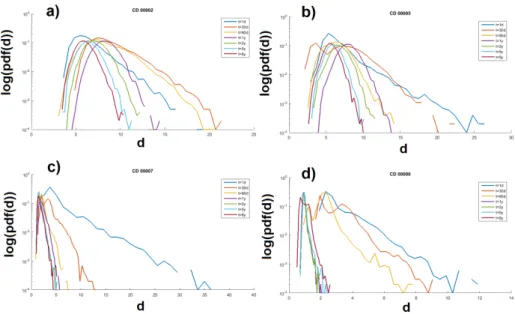
ysis of the distributions of d, shown in Figure 3, provides further insights on this behaviour.
159
Taking C=0.002 as example, one can see a clear shift of the distribution toward larger
160
values in going from daily to monthly values.
On the contrary, averaging beyond 1 year time-scales suppresses the extreme d
val-162
ues in the tails of the distributions, which corresponds to a smoothing of the
variabil-163
ity of the dimension, thus lowering hdi. This is particularly evident for the case of C=0.007
164
and C=0.008 (LFV runs) and should be expected since there is a smoothing of the
vari-165
ability on the attractor (Figure 1 b, d, f, h). This smoothing removes specific
frequen-166
cies in the dynamics, as discussed in details in Nicolis and Nicolis [1995]; Vannitsem and
167
Nicolis [1995, 1998], and also reduces the local variability of the instability properties
168
of the flow. Another interesting result is that at monthly and seasonal scales the
distri-169
butions of d display a double peak for runs both with and without LFV (Figure 4). This
170
double peak is associated with the seasonal variability; there is a dominance of large d
171
in Winter and low d in Summer. For instance for C=0.005, there is a maximum around
172
d = 8 for the winter conditions and d = 4 for summer conditions (Figure 4) . To
in-173
terpret this feature one must recall that the large-scale winter dynamics in the mid-latitudes
174
is driven by a larger gradient of equator-to-pole radiative input than in summer [Goosse,
175
2015; Vannitsem, 2015, 2017]. This has strong implications for the instability
proper-176
ties of the flow [Buizza and Palmer , 1995]. This is also a property of the coupled
ocean-177
atmosphere model used here, which displays lower averaged local Lyapunov exponents
178
(and averaged local Lyapunov dimensions) in Summer than in Winter [Vannitsem, 2017].
179
The technique we adopt here succesfully captures this increase in the complexity of the
180
dynamics. The distributions further highlight the fact that, in some cases, the average
181
of d remains roughly constant but the positive tails of the distributions change radically.
182
This suggests that a decrease in hdi due to averaging might change little in the system’s
183
ground state while altering the configurations with the largest number of degrees of
free-184
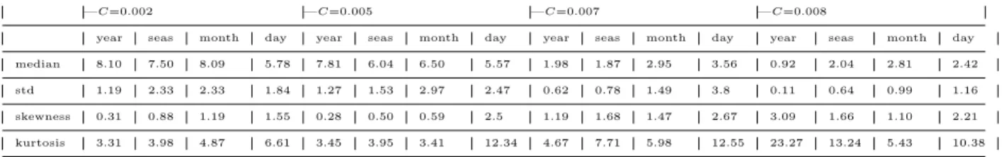
dom. Table 1 reports the values of the first four moments of the distribution of d for all
185
C and averaging times.
186
One can further wonder whether hdi are determined predominantly by the oceanic
187
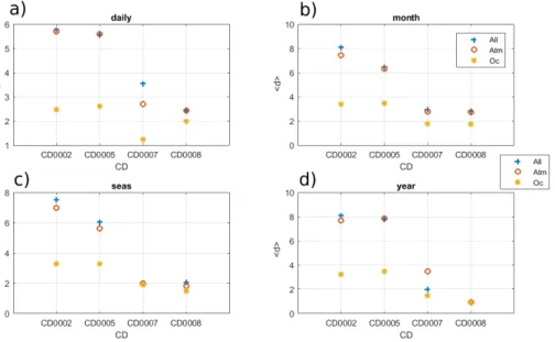
or the atmospheric modes. To do this, we compute the local dimensions of the oceanic
188
and atmospheric components separately. The results are shown in Figure 5 for different
189
averaging periods. Except for the C=0.007 case, the atmospheric modes alone return
al-190
most the same value of the total dimension as the joint calculation. The analysis of the
191
ocean variables instead gives a lower dimension. This interesting feature likely reflects
192
the fact that, although the ocean variables are coupled to the atmosphere, they only
re-193
tains part of the complex structure of the system, in particular for the low values of C.
In our view, this results from the fact that the dynamics in the ocean is only ”weakly”
195
driven by the chaotic variability present in the atmosphere for small values of C due to
196
the large inertia of the ocean that integrates the atmospheric forcing on long time scales.
197
For large values of C, LFV develops and this effect is considerably weakened; variables
198
from both components then provide similar results. However, the behavior observed for
199
C = 0.007 is still slightly non-monotonic because this run still gives a chaotic
attrac-200
tor, whereas the run C = 0.008 provide a quasi-periodic flow.
201
5 Implications for Ocean-Atmosphere Coupling and conclusions
202
In the present study we have investigated the effects of time averaging on the
ocean-203
atmosphere system as represented by a conceptual coupled model. The impact of
aver-204
aging is quantified in terms of changes in the attractor properties of the system. When
205
the averaging time is increased, the local dimension shows a non-monotonic behaviour
206
for short averaging times, but ultimately decreases for windows longer than 1 year. For
207
these averaging windows, the distribution of the local dimension becomes closer to
Gaus-208
sian and the variability decreases. This corresponds to a progressive smoothing of the
209
attractor. Time-averaging therefore has profound and sometimes counter-intuitive
im-210
plications for the dynamical characteristics of climate data. Our results also suggest that,
211
on longer time scales, the climate dynamics is smoother and closer to that of
homoge-212
nous, hyperbolic systems.
213
It is however necessary to verify whether the results from the idealised model
pre-214
sented above find a match in real-world data. Here, we repeat our analysis for El
Nino-215
Southern Oscillation Nino3 and North Atlantic Oscillation (NAO) indices. As a caveat,
216
we note that this analysis has an important difference from that of the full coupled model.
217
Indeed, the NAO and Nino3 indices do not represent the full climate attractor whereas
218
they can be thought of as a projection (a special Poincar´e section) of the full
dynam-219
ics. In this sense the analysis can still inform us on numerous aspects of the system (see
220
for example Faranda et al. [2017c] for a similar argument on the Von Karmann
turbu-221
lent swirling flow). A separate problem to consider is the length of the time series, as
222
our method for computing the local dimensions is dependent on processing a sufficiently
223
long series. The shortest timeseries we analyse are the yearly ones, for which we only
dis-224
pose of 947 years; we therefore perform two different computations of the dimension: i)
225
for each dataset we use the complete timeseries, ii) for each dataset we only use 947 data
points. This provides some indication of the robustness of our conclusions. The results
227
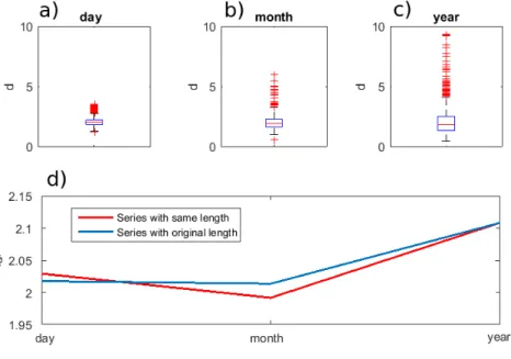
are reported in Figure 6. The top panels show the boxplot of the local dimension
dis-228
tributions when all the data are considered, whereas the lower panel presents the
aver-229
age dimension for the two cases described. The analysis of the boxplots suggest that the
230
extremes of d change with the time scale considered. For the yearly time series, we
ob-231
tain values of d up to 10. This may seem nonphysical since we are only analyzing two
232
time series but, following again Faranda et al. [2017c], can be understood by
consider-233
ing the role of small scale turbulence in increasing the effective dimension of the
attrac-234
tor. Sampling issues may be discarded because both the full and reduced datasets show
235
comparable relative changes between the different temporal resolutions. Finally the
non-236
monotonic behavior of the average dimension for the climate indices follows the one found
237
in the coupled model. We therefore conclude that the inferences drawn from the
con-238
ceptual model provide valuable insights into the behaviour of real-world climate data and
239
should be considered when performing dynamical analyses of data with low temporal
res-240
olutions. It is worth performing further analysis in more sophisticated climate models
241
in order to clarify in particular the increase of variability of the local dimension found
242
in Figure 6. For that, very long (historical) runs should be considered in order to have
243
enough data for the extreme value analysis, provided that climate models can correctly
244
reproduce the internal variability of the climate system.
245
6 Acknowledgments
246
D. Faranda and G. Messori were supported by ERC grant No. 338965. The work
247
of St´ephane Vannitsem is partly supported by the Belgian Federal Science Policy under
248
contract BR/165/A2/Mass2Ant. G. Messori was also supported by the Swedish Research
249
Council under contract: 2016-03724
250
References
251
Baehr, J., K. Fr¨ohlich, M. Botzet, D. I. Domeisen, L. Kornblueh, D. Notz, R.
Pi-252
ontek, H. Pohlmann, S. Tietsche, and W. A. Mueller (2015), The prediction of
253
surface temperature in the new seasonal prediction system based on the mpi-esm
254
coupled climate model, Climate Dynamics, 44 (9-10), 2723–2735.
255
Barnston, A. G., and R. E. Livezey (1987), Classification, seasonality and
persis-256
tence of low-frequency atmospheric circulation patterns, Monthly weather review,
115 (6), 1083–1126.
258
Bond, G., B. Kromer, J. Beer, R. Muscheler, M. N. Evans, W. Showers, S.
Hoff-259
mann, R. Lotti-Bond, I. Hajdas, and G. Bonani (2001), Persistent solar influence
260
on north atlantic climate during the holocene, Science, 294 (5549), 2130–2136.
261
Buizza, R., and T. Palmer (1995), The singular-vector structure of the atmospheric
262
global circulation, Journal of the Atmospheric Sciences, 52 (9), 1434–1456.
263
Cane, M. A., S. E. Zebiak, and S. C. Dolan (1986), Experimental forecasts of el
264
nino, Nature, 321 (6073), 827.
265
Dalcher, A., and E. Kalnay (1987), Error growth and predictability in operational
266
ecmwf forecasts, Tellus A: Dynamic Meteorology and Oceanography, 39 (5), 474–
267
491.
268
Faranda, D., V. Lucarini, G. Turchetti, and S. Vaienti (2011), Numerical
conver-269
gence of the block-maxima approach to the generalized extreme value distribution,
270
Journal of statistical physics, 145 (5), 1156–1180.
271
Faranda, D., G. Messori, and P. Yiou (2017a), Dynamical proxies of north atlantic
272
predictability and extremes, Scientific reports, 7, 41,278.
273
Faranda, D., G. Messori, M. C. Alvarez-Castro, and P. Yiou (2017b), Dynamical
274
properties and extremes of northern hemisphere climate fields over the past 60
275
years, Nonlinear Processes in Geophysics, 24 (4), 713.
276
Faranda, D., Y. Sato, B. Saint-Michel, C. Wiertel, V. Padilla, B. Dubrulle, and
277
F. Daviaud (2017c), Stochastic chaos in a turbulent swirling flow, Physical review
278
letters, 119 (1), 014,502.
279
Freitas, A. C. M., J. M. Freitas, and M. Todd (2010), Hitting time statistics and
280
extreme value theory, Probability Theory and Related Fields, 147 (3-4), 675–710.
281
Goosse, H. (2015), Climate System Dynamics and Modeling, Cambridge University
282
Press.
283
Huang, B., P. W. Thorne, V. F. Banzon, T. Boyer, G. Chepurin, J. H. Lawrimore,
284
M. J. Menne, T. M. Smith, R. S. Vose, and H.-M. Zhang (2017), Extended
recon-285
structed sea surface temperature, version 5 (ersstv5): upgrades, validations, and
286
intercomparisons, Journal of Climate, 30 (20), 8179–8205.
287
Jones, P., T. Jonsson, and D. Wheeler (1997), Extension to the north atlantic
os-288
cillation using early instrumental pressure observations from gibraltar and
south-289
west iceland, International Journal of climatology, 17 (13), 1433–1450.
Lorenz, E. (1982), Atmospheric predictability experiments with a large numerical
291
model, Tellus, 34 (6), 505–513.
292
Lorenz, E. N. (1969), The predictability of a flow which possesses many scales of
293
motion, Tellus, 21 (3), 289–307.
294
Lovejoy, S., D. Schertzer, and J. Stanway (2001), Direct evidence of multifractal
295
atmospheric cascades from planetary scales down to 1 km, Physical review letters,
296
86 (22), 5200.
297
Lucarini, V., D. Faranda, and J. Wouters (2012), Universal behaviour of extreme
298
value statistics for selected observables of dynamical systems, Journal of statistical
299
physics, 147 (1), 63–73.
300
Lucarini, V., D. Faranda, A. C. M. Freitas, J. M. Freitas, H. Mark, K. Tobias,
301
M. Nicol, M. Todd, and S. Vaienti (2016), Extremes and recurrence in
dynami-302
cal systems.
303
Mann, M. E., Z. Zhang, S. Rutherford, R. S. Bradley, M. K. Hughes, D. Shindell,
304
C. Ammann, G. Faluvegi, and F. Ni (2009), Global signatures and dynamical
305
origins of the little ice age and medieval climate anomaly, Science, 326 (5957),
306
1256–1260.
307
Messori, G., R. Caballero, and D. Faranda (2017), A dynamical systems approach
308
to studying midlatitude weather extremes, Geophysical Research Letters, 44 (7),
309
3346–3354.
310
Nicolis, C., and G. Nicolis (1995), From short-scale atmospheric variability to global
311
climate dynamics: toward a systematic theory of averaging, Journal of the
atmo-312
spheric sciences, 52 (11), 1903–1913.
313
Palmer, T. N., and D. L. Anderson (1994), The prospects for seasonal forecasting–a
314
review paper, Quarterly Journal of the Royal Meteorological Society, 120 (518),
315
755–793.
316
Pedlosky, J. (2013), Geophysical fluid dynamics, Springer Science & Business Media.
317
Pouquet, A., and R. Marino (2013), Geophysical turbulence and the duality of the
318
energy flow across scales, Physical review letters, 111 (23), 234,501.
319
Reynolds, R. W., T. M. Smith, C. Liu, D. B. Chelton, K. S. Casey, and M. G.
320
Schlax (2007), Daily high-resolution-blended analyses for sea surface
tempera-321
ture, Journal of Climate, 20 (22), 5473–5496.
Trouet, V., J. Esper, N. E. Graham, A. Baker, J. D. Scourse, and D. C. Frank
323
(2009), Persistent positive north atlantic oscillation mode dominated the medieval
324
climate anomaly, science, 324 (5923), 78–80.
325
Vannitsem, S. (2015), The role of the ocean mixed layer on the development of the
326
north atlantic oscillation: A dynamical system’s perspective, Geophysical Research
327
Letters, 42 (20), 8615–8623.
328
Vannitsem, S. (2017), Predictability of large-scale atmospheric motions: Lyapunov
329
exponents and error dynamics, Chaos: An Interdisciplinary Journal of Nonlinear
330
Science, 27 (3), 032,101.
331
Vannitsem, S., and M. Ghil (2017), Evidence of coupling in ocean-atmosphere
dy-332
namics over the north atlantic, Geophysical Research Letters, 44 (4), 2016–2026.
333
Vannitsem, S., and V. Lucarini (2016), Statistical and dynamical properties of
co-334
variant lyapunov vectors in a coupled atmosphere-ocean modelmultiscale effects,
335
geometric degeneracy, and error dynamics, Journal of Physics A: Mathematical
336
and Theoretical, 49 (22), 224,001.
337
Vannitsem, S., and C. Nicolis (1995), Dynamics of fine scale variables versus
aver-338
aged observables in a simplified thermal convection model, Journal of Geophysical
339
Research: Atmospheres, 100 (D8), 16,367–16,375.
340
Vannitsem, S., and C. Nicolis (1998), Dynamics of fine-scale variables versus
av-341
eraged observables in a t21l3 quasi-geostrophic model, Quarterly Journal of the
342
Royal Meteorological Society, 124 (551), 2201–2226.
343
Vannitsem, S., J. Demaeyer, L. De Cruz, and M. Ghil (2015), Low-frequency
vari-344
ability and heat transport in a low-order nonlinear coupled ocean–atmosphere
345
model, Physica D: Nonlinear Phenomena, 309, 71–85.
346
Vinther, B. M., P. Jones, K. Briffa, H. Clausen, K. Andersen, D. Dahl-Jensen, and
347
S. Johnsen (2010), Climatic signals in multiple highly resolved stable isotope
348
records from greenland, Quaternary Science Reviews, 29 (3), 522–538.
Table 1. Moments of the distributions of d for different C and averaging times.
350
—C=0.002 —C=0.005 —C=0.007 —C=0.008
year seas month day year seas month day year seas month day year seas month day median 8.10 7.50 8.09 5.78 7.81 6.04 6.50 5.57 1.98 1.87 2.95 3.56 0.92 2.04 2.81 2.42 std 1.19 2.33 2.33 1.84 1.27 1.53 2.97 2.47 0.62 0.78 1.49 3.8 0.11 0.64 0.99 1.16 skewness 0.31 0.88 1.19 1.55 0.28 0.50 0.59 2.5 1.19 1.68 1.47 2.67 3.09 1.66 1.10 2.21 kurtosis 3.31 3.98 4.87 6.61 3.45 3.95 3.41 12.34 4.67 7.71 5.98 12.55 23.27 13.24 5.43 10.38
Figure 1. Poincar´e sections for the modes 2,9,15. Different couplings a,c,e,g): C=0.002. b,d,f,h) C=0.007. Different averaging windows: a,b) daily; c,d) monthly; e,f) yearly; g,h) 8 years averages.
351
352
Figure 2. Average local dimensions as a function of the coupling and the averaging window.
354
Figure 3. Attractor dimensions’ distributions as a function of the coupling and the averaging window. a) C=0.002, b) C=0.005, c) C=0.007, d) C=0.008
355
356
Figure 4. Attractor dimensions’ distributions as a function of the coupling for monthly (a) and seasonal (b) averaging time.
357
358
Figure 5. Average dimensions hdi computed selecting all modes (blue stars) atmospheric modes only (red crosses), oceanic modes only (yellow triangles). a) daily, b) monthly, c) seasonal and d) yearly data.
359
360
Figure 6. a,b,c): boxplots of local dimensions d for NAO and Nino3 indices at different time scales. On each box, the central mark is the median, the edges of the box are the 25th and 75th percentiles, the whiskers extend to the most extreme data points not considered outliers, and outliers are plotted individually. a) daily, b) monthly and c) yearly data. d): average dimension hdi computed with the full length time-series (blue) and only 947 time steps (red).
362
363
364
365