Impact of the en echelon fault connectivity on reservoir flow simulations

(1)

HAL Id: hal-01281809

https://hal.univ-lorraine.fr/hal-01281809

Submitted on 27 Feb 2018

HAL is a multi-disciplinary open access

archive for the deposit and dissemination of sci-entific research documents, whether they are pub-lished or not. The documents may come from

L’archive ouverte pluridisciplinaire HAL, est destinée au dépôt et à la diffusion de documents scientifiques de niveau recherche, publiés ou non, émanant des établissements d’enseignement et de

Impact of the en echelon fault connectivity on reservoir

flow simulations

Charline Julio, Guillaume Caumon, Mary Ford

To cite this version:

Charline Julio, Guillaume Caumon, Mary Ford. Impact of the en echelon fault connectivity on reservoir flow simulations. Interpretation, American Association of Petroleum Geologists, Society of Exploration Geophysicists, 2015, 3 (4), pp.SAC23-SAC34. �10.1190/INT-2015-0060.1�. �hal-01281809�

(2)

IMPACT OF THE EN-ECHELON FAULT

1

CONNECTIVITY ON RESERVOIR FLOW

2

SIMULATIONS

3

Charline Julio

1

, Guillaume Caumon

1,*

, and Mary Ford

2

4

1_{GeoRessources, Universit´}_{e de Lorraine-ENSG/CNRS/CREGU, 2 rue du Doyen Marcel} 5

Roubault, Vandoeuvre-l`es-Nancy F-54518, France

6

2_{CRPG, Universit´}_{e de Lorraine-ENSG/CNRS, 15 Rue Notre Dame des Pauvres,} 7

Vandoeuvre-l`es-Nancy F-54501, France

8

*_{Corresponding author. Tel.: +333 83 59 64 40. Fax: +333 83 59 64 60. E-mail} 9 address: Guillaume.Caumon@ensg.univ-lorraine.fr 10

July 10, 2015

11 Abstract 12

Limited resolution and quality of seismic data and time requirements for

13

seismic interpretation can prevent a precise description of the connections

14

between faults. We focus on the impact of the uncertainties related to the

15

connectivity of en-echelon fault arrays on fluid flow simulations. We use a

16

set of one hundred different stochastic models of the same en-echelon fault

17

array. These fault array models vary in number of relay zones, relative

posi-18

tion of fault segments, size of overlap zones and number of relay faults. We

(3)

automatically generate a flow model from each fault array model in four main

20

steps: (1) stochastic computation of relay fault throw, (2) horizon building,

21

(3) generation of a flow simulation grid, and (4) definition of the static and

22

dynamic parameters. Flow simulations performed these stochastic fault

mod-23

els with deterministic petrophysical parameters entail significant variability

24

of reservoir behavior, which cannot always discriminate between the types of

25

fault segmentation. We observe that the simplest interpretation consisting

26

of one fault significantly yields significantly biased water cut forecasts at

pro-27

duction wells. This highlights the importance of integrating fault connectivity

28

uncertainty in reservoir behavior studies.

29

Introduction

30

During the interpretation of compartmentalized reservoirs, the characterization

31

of fault connectivity is often critical to match production history and make

reason-32

able forecasts of reservoir performance (e.g., Jolley et al. (2007)). In this context,

33

fault connectivity concerns not only the large-scale pattern of faults, which can

34

originate from several tectonic episodes (Sanderson and Nixon, 2015), but also the

35

phenomenon of en-echelon faults, which results from the growth, overlap and linkage

36

of several fault segments, see for instance Peacock and Sanderson (1991); Cowie and

37

Scholz (1992); Cartwright et al. (1995); Childs et al. (1995); Fossen and Hesthammer

38

(2000); Walsh et al. (2003); Giba et al. (2012).

39

In the subsurface, the characterization of these zones typically relies of 3D

seis-40

mic data but may be limited by the seismic resolution and artifacts (Thore et al.,

41

2002). Indeed, the relatively wide damage zones around overlapping fault segments

42

(Kim et al., 2004; Rotevatn et al., 2007) tends to diffract seismic waves and make

(4)

relay fault interpretations very delicate. Significant literature about the description

44

and statistics about en-echelon fault arrays may be used to drive the fault segment

45

identification (e.g., Cartwright et al. (1995); Walsh et al. (2003); Soliva and

Bene-46

dicto (2004)). However, in practice, limited interpretation time is also a source of

47

uncertainties, which can be exacerbated by the insufficient use of geological concepts

48

(Kattenhorn and Pollard, 2001; Bond et al., 2007; Bond, 2015).

49

The impact of fault overlap zones on reservoir behavior has been studied by

sev-50

eral authors (Bense and Van Balen, 2004; Micarelli et al., 2006; Manzocchi et al.,

51

2008a; Rotevatn et al., 2009a,b; Manzocchi et al., 2010; Fachri et al., 2013). Relay

52

zones are often described as flow conduits between two fault blocks which would

53

otherwise be isolated (Bense and Van Balen, 2004; Manzocchi et al., 2010).

How-54

ever, the complexity and diversity of relay zones make it very challenging to define

55

a general quantitative rule about their impact on fluid flow (Manzocchi et al., 2010;

56

Bastesen and Rotevatn, 2012). Indeed, the overlap zones are usually associated with

57

intense brittle deformation that can lead to the formation of a relay fault. Figure 1a

58

shows a simplified view of a relay fold, which may be affected by fractures and

com-59

paction bands, while Figure 1b shows a more mature structure where the relay has

60

been breached by a relay fault. These two configurations correspond to soft-linked

61

segments (Figure 1a) and hard-linked segments (Figure 1b). Such relay structures

62

can act as barriers or drains depending on the fluid types, the rock nature and the

63

amount and type of deformation. Geometrically, the existence or absence of a

con-64

necting breach fault in an overlap zone can have a large effect on the juxtaposition

65

of stratigraphic units on either sides of the fault zone. As a first approximation,

66

the juxtaposition of two high permeability units increases the connectivity between

67

two fault blocks, whereas a reservoir unit can be sealed due to its juxtaposition

(5)

with low permeability units. However, more complex effects can occur due to the

69

possible occurrence of cataclasic deformation bands or the smearing of shale in the

70

fault planes.

71

Representing the effects of all these features of reservoir flow model is

challeng-72

ing, especially for multi-phase flow, see Manzocchi et al. (2010). A possible avenue

73

is to integrate the effects of these features as deterministic or stochastic

perturba-74

tions of transmissibilities between neighboring control volumes in the flow simulation

75

grid. For example, Manzocchi et al. (2008a) capture the effects of small fault throw

76

changes in a pillar-based reservoir grid and simulate relay zone frequency based on

77

the mapped throw. In this paper, we instead explicitly create a new grid for each

78

realization to capture the uncertainties.

79

For this, we build on a recent stochastic method that generates a set of possible

80

segmentation configurations from a composite fault interpreted as one continuous

81

structure (Julio et al., 2015). A segmentation configuration means here a 3D

ge-82

ometric model composed of overlapping segments separated by breached or intact

83

relay zones. The method uses the orientation variations of the composite fault as

84

indicators of the occurrence of relay zones. The models generated by this method

85

mainly vary in number of fault segments, relative position of the segments, size of

86

overlap zones and number of relay faults. From each fault model and horizon data,

87

we create a synthetic numerical flow model made of a flow simulation grid associated

88

with static and dynamic parameters.

89

As compared to transmissibility-based approaches, our method is not a priori

90

constrained by a reference flow simulation grid and allows considering the effects of

91

fault segments on the static accumulations. It probably allows for more variability

92

in the simulated geometry of relay zones, by exploiting the capabilities of recent

(6)

advanced gridding algorithms to integrate more complex fault descriptions than

94

generally possible in pillar grids (Gringarten et al., 2008; Mallison et al., 2014). We

95

also believe such an explicit geometric representation could be interesting in the

96

future to integrate the effects of juxtaposition and damage zones on other physical

97

processes (e.g., geomechanics or seismic wave propagation). In the context of the

98

present paper which uses stair-step corner-point geometry flow grids, the method is

99

suitable for local flow models or global flow models in which the separation between

100

fault segments is larger than the areal grid resolution, as for instance in Rotevatn

101

et al. (2009a).

102

In the following, we present the method to stochastically simulate relay zones and

103

apply it to a reservoir model. Our approach extends the previous work by Julio et al.

104

(2015). In particular, we capture the fault juxtaposition uncertainties in the relay

105

zones by simulating possible throws of the relay fault, and we generate grids whose

106

topology and geometry may vary for each realization. This allows us to perform

107

a flow sensitivity analysis on all the simulated models to study the relationships

108

between the types of segments and the flow behavior.

109

[Figure 1 about here.]

110

Automatic generation of segmented reservoir

mod-111

els

112

Reservoir modeling generally aims at transforming geophysical and borehole

in-113

terpretations into a 3D reservoir flow grid. Standard workflows are roughly

com-114

posed of four main successive steps. (1) The first step consists of building a reservoir

115

structural model in which the geological interfaces, such as faults, horizons and

(7)

conformities, are represented as 3D surfaces (Mallet, 1988; Caumon et al., 2009).

117

(2) Then, a corner-point grid widely used in reservoir simulation provide a 3D mesh

118

of the reservoir volume. (3) From well data, the petrophysical properties of the rock

119

are computed using deterministic interpolations or stochastic simulations (Pyrcz and

120

Deutsch, 2014). (4) Flow simulations may then be finally performed based on finite

121

volume methods.

122

In this paper, we combine a new method to create a stochastic description of

123

a 3D segmented fault (Julio et al., 2015) with standard existing methods for the

124

steps 1-3. This section starts with a description of the data set used in our study

125

and generated by the method of Julio et al. (2015). Then, we present the strategy

126

applied to model the horizons. Indeed, as no horizon data points are available in

127

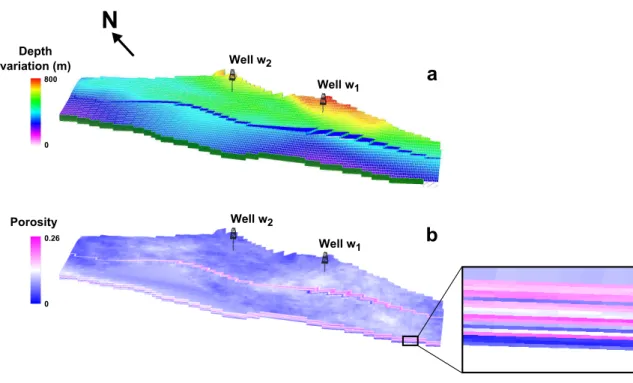
relay zones, we propose to stochastically estimate the throw of the relay faults, and

128

to use this estimation to constrain the interpolation of the horizon geometry in relay

129

zones. Then, we explain how we create a conventional reservoir simulation grid for

130

each of the stochastic structural models.

131

Data set and stochastic fault model generation

132

The proposed method is applied on a Middle East case study whose orientation,

133

reservoir depth and fluid contact depth have been modified for confidentiality

rea-134

sons. The data set used to model the reservoir is composed of: two horizon point sets

135

and a normal fault F (Figure 2). The two horizon point sets and the fault F have

136

been interpreted from a relatively low-quality onshore 3D seismic data set. These

137

two horizons delimit a reservoir formation whose thickness is about 180 m and cover

138

an area of 11 km by 1.1 km. The faultF is a composite normal fault whose

segmenta-139

tion could not be clearly identified from the seismic data. The global geometry of the

(8)

reservoir is a monoclinal horst striking N 140 (Figure 2). The faultF strikes parallel

141

to the main reservoir orientation and may be a potential flow barrier between the

142

upper compartment and the lower compartment whose pressure is supported by an

143

active aquifer located in the SW. The uncertainties associated to the exact location

144

of this fault can also impact the OOIP because the top depth of footwall block is

145

close to the oil-water contact depth. Therefore, small fault throw perturbation has

146

a relatively large impact on reservoir closure. In the reservoir zone, the orientation

147

of the faultF locally shows some abrupt variations in the strike direction.

148

Julio et al. (2015) quantify these strike variations and interpret them as possible

149

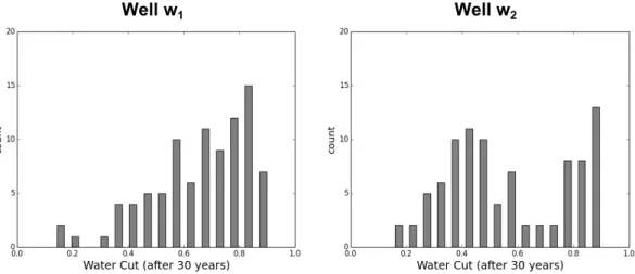
indicators of overlap zone occurrence. Their stochastic simulation method simulates

150

possible fault segments from approximately planar areas in the fault surface using

151

probabilistic descriptions about relative segment size and overlap/size relationships.

152

This method has been applied to generate one hundred segmentation models of the

153

faultF. These models may have different number of fault segments, size of overlap

154

zones, relative position of segments and segment geometry. The occurrence or not

155

of a relay fault in an overlap zone is determined from the ratio between overlap

156

(overlap zone length) and separation (overlap zone width). If this ratio is superior

157

to a stochastically-chosen threshold, a relay fault is modeled in the middle of the

158

corresponding overlap zone (Soliva and Benedicto, 2004). In the vertical direction,

159

the relay faults have the same extent as the associated overlapping segments. Figure

160

3 summarizes the generated configurations among the one hundred downscaled

mod-161

els of the fault F. The three main obtained segmentation configurations are: 28%

162

are two hard-linked left-stepping segments, 25% are two soft-linked right-stepping

163

segments, 16% are three soft-linked segments (Figure 3).

164

The downscaling method introduced by Julio et al. (2015) deals only with the

(9)

uncertainty related to faults (treated as slip surfaces), without consideration of the

166

displacement in the relay zone that may be poorly-imaged on the seismic data.

167

Therefore, we now present a new algorithm to manage uncertainties on the throw

168

of relay faults, which can have a large impact on flow (Manzocchi et al., 2010).

169

170

171

Stochastic computation of relay fault throws

172

3D horizons are built by interpolation of input point sets extracted from 3D

173

seismic data. However, in the majority of cases, the low quality of seismic data does

174

not allow the characterization of the horizon geometry in overlap zones. In models

175

with a continuous ramp in the relay, the geometry is computed by interpolation

176

between horizon picks available on either side of the ramp. This is essentially similar

177

to making a thin-plate assumption of the horizon geometry within the relay ramp.

178

In models where the ramp is breached, the relay fault throw must be estimated

179

before interpolating the horizon geometry.

180

For this, we propose to simulate points that will be used as interpolation

con-181

straints for horizon building in breached relay zones. Consider a horizon denoted

182

H and a relay fault denoted R. The method computes the vertical displacement

183

(denoted d) of the horizon H in the neighborhood of the relay zone, i.e. the total

184

displacement away from the relay faultR. This displacement d is computed from a

185

sphere centered on the relay fault center and whose radius is input by the interpreter

186

(Figure 4). The points associated with the horizon H inside the sphere are selected

187

and the algorithm differentiates the points located in the footwall of the relay fault

(10)

from the ones in the hanging wall. The mean difference in depth between these two

189

point sets gives an estimate of the vertical displacement d. If the sphere contains

190

no data point, it is enlarged until points are found. This methodology calls for

reli-191

able horizon picks in the vicinity of the fault, for example by eliminating potentially

192

erratic points within a certain distance of the fault surface.

193

The vertical displacement d corresponds to the sum of the throw (dF ault) of the

194

relay faultR and of the vertical displacement (dF old) associated with the ramp fold,

195

which is also termed “throw deficit” (Faure Walker et al., 2009). The ratio between

196

the relay fault throw dF ault and the total displacement d at the relay fault center

197

is related to the maturity of the relay zone. In our method, we use a probability

198

distribution from which this ratio can be sampled to generate a particular realization.

199

In the vertical direction, this ratio is assumed to be maximal at the relay fault center

200

and to decrease vertically towards the relay fault tips. Consider a function β that

201

characterizes the ratio evolution (Figure 4a), and a parameter v that is the signed

202

difference between the relay fault center depth and the mean depth of the horizon

203

H inside the sphere. The value of the relay fault throw associated with the horizon

204

H is defined as:

205

dF ault = β(v) · d (1)

The hanging wall and the footwall may differently accommodate the brittle

defor-206

mation. Therefore, we define a partition factor γ (between 0 and 1) as the proportion

207

of throw accommodated by the footwall (Georgsen et al., 2012; Laurent et al., 2013).

208

Thus, the values of throw in the footwall and in the hanging wall are:

209

(11)

210

dHAN G_{F ault} = (1 − γ) · dF ault (3)

The values dF OOT

F ault and dHAN GF ault are used to add synthetic horizon points

condition-211

ing the relay fault throw (Figure 4b). These new stochastic points and the initial

212

point sets are used to interpolate the horizon geometry (Figure 4b). In terms of

213

impact of these parameters, the value of β directly affects the geometry and the

214

juxtaposition of rock units across the fault zone. The value of γ has probably less

215

influence because if only affects the depth of the layers in the fault zone and not the

216

juxtaposition.

217

In our application, the parameter β(0) characterizing the ratio between the relay

218

fault throw and the total vertical displacement at the fault center is randomly chosen

219

from a Gaussian distribution defined by a mean and a standard deviation equal to

220

0.5 and 0.08, respectively. This means that the relative throw deficit due to the relay

221

is assumed to vary between 34% and 56% of the global throw d in 95 % of the cases.

222

The choice of these values are here arbitrary, so further studies should be made to

223

define β(0) according to the lithology and to the intensity of the deformation. The

224

partition factor γ is also chosen from a Gaussian distribution defined by a mean and

225

a standard deviation equal to 0.5 and 0.08, respectively. Indeed, as the relay faults

226

have been simulated in the middle of the overlap zones, we make the parsimonious

227

assumption that, on average, the footwall and the hanging wall accommodate about

228

the same quantity of deformation.

229

(12)

Grid computation and petrophysical modeling

231

Based on the API (Application Programming Interface) of the geomodeling

soft-232

ware Gocad-SKUA, we have developed a plugin which implements the stochastic

233

segmented fault downscaling approach described above and then automatically

gen-234

erates a corner-point grid honoring these structures (Figure 5a). The gridding

235

method generates stair-step corner-point grids as described in Gringarten et al.

236

(2008). Essentially, the reservoir grids honor the stratigraphic layering and

main-237

tain sub-orthogonal cell shapes suitable for conventional reservoir simulation. As a

238

result, the faults are discretized as stair-step cell faces.

239

This allows us to efficiently build grids from a large set of stochastic structural

240

models. The grid dimensions are globally equal to 11 km × 3 km × 0.8 km. Each

241

grid is composed of the same number of cells (230 × 30 × 20 = 230, 000), yielding

242

an average grid block size of 48 × 122 × 8.6 m. However, due to the topological and

243

geometrical changes of the fault array, the number of active cells slightly varies in

244

each model and is approximately equal to 112,000 (cells are considered dead if their

245

pore volume is lower than 100 m3).

246

To isolate the effect of fault uncertainty on flow behavior, we have used the same

247

synthetic petrophysical model in all the simulated grids. This petrophysical model

248

assumes laterally continuous but vertically layered rock types as could exist for

in-249

stance in turbiditic lobes. The Net-To-Gross values have been chosen constant and

250

equal to 0.8. The porosity and the permeability have been simulated as stationary

251

Gaussian random fields using a Sequential Gaussian Simulation (Figure 5b). We

252

used spherical variogram models with ranges of 5 km, 3 km and 5 m in the N 140,

253

N 230 and vertical directions, respectively. The porosity approximately follows a

(13)

normal distribution of average 0.13 and standard deviation 0.02. The horizontal

255

permeability is isotropic and approximately follows a triangular distribution of

min-256

imum 200 mD, mode 600mD and maximum 1500mD. It has a 0.98 rank correlation

257

coefficient with the porosity values. The KV/KH ratio is taken constant and equal

258

to 0.001 to compensate for the relatively coarse vertical grid resolution.

259

Flow simulations results and interpretations

260

Fluid flow simulation parameters

261

The en-echelon fault array completely crosses the reservoir from NW to SE

(Fig-262

ure 5). The faults are considered as partially sealing with transmissibility multipliers

263

assumed constant and equal to 0.05.

264

Two initial fluids, water and oil, are initially present in the reservoir. The initial

265

water saturation in the oil zone is 0.05 and the residual oil saturation after water

266

flooding is 0.24. The water oil contact vertically crosses the fault array (Figures 6

267

and 7). At the SW, an aquifer maintains the reservoir pressure during oil production

268

(Table 1).

269

The reservoir production scenario takes advantage of aquifer pressure support

270

and only uses two production wells w1 and w2, located in the NE near the top of the

271

structure (Figure 5, Table 1). In the initial state, all the well perforations are located

272

in the oil zone. The wells are controlled by the oil production rate but completions

273

may be shut down if the bottom-hole becomes lower than an input threshold (Table

274

1).

275

(14)

277

278

[Table 1 about here.]

279

Fault segmentation impact on flow simulations

280

From the 100 downscaled models, we obtained 93 flow simulations. The seven

281

other models failed during the automatic grid generation step or the flow simulations.

282

In this section, we compare the oil saturation and the water cut evolution of the

283

different segmented reservoir models (Figures 9, 7, 10, 11).

284

Range of initial conditions. The stochastic estimate of relay fault throws and

285

the interpolation between point sets involve some variations on the initial oil in place

286

value of the stochastic downscaled models. The mean and the standard deviation

287

are equal to 176.8 M sm3 and 1.710 M sm3, respectively (Figure 8). These variations

288

can be explained because the local throw and reservoir top depth variations directly

289

affect the gross rock volume above the oil-water contact. The model composed of

290

the single faultF (177.3 Msm3_{) is close to the mean (Figure 8).}

291

292

Range of dynamic responses. After 30 years of production, the water cut values

293

vary from 0.13 to 0.91 in well w1 and from 0.15 to 0.91 in well w2 (Figure

10a-294

b). This very high dispersion of water-cuts highlights the significant impact of

295

fault segmentation on reservoir behavior. In the reservoir model composed of the

296

continuous faultF (before downscaling), the water-cut values are respectively equal

(15)

to 0.37 and 0.85 in wells w1 and w2 after 30 years of production (Figure 9). These 298

two values are close to the extreme values of the statistics of downscaled models.

299

Indeed, the deterministic water cut value (0.37) for the well w1 is inferior to the

300

10th percentile (0.43) of the stochastic models, and, on contrary, the deterministic

301

water cut value (0.85) for the well w2 is superior to the 80th percentile (0.81) of

302

the stochastic models. Thus, performing flow simulations on the fault F without

303

consideration of the segmentation uncertainties may lead to major approximations

304

in dynamic behavior predictions, and therefore in oil production estimates.

305

Fault segmentation configurations and flow responses. One of the outputs

306

of the downscaling method is the probability of segmentation configurations (Figure

307

3). These configurations can be seen as samples of discrete structural scenarios.

308

Could these scenarios be discriminated from actual reservoir production data? To

309

answer this question, for each of these configurations, we analyze the water cut

310

evolution and the breakthrough time (considered occurring when the water fraction

311

reaches 0.01 at producer wells).

312

Figure 10c-d shows the evolution for models composed of two hard-linked

left-313

stepping segments and of two soft-linked right-stepping segments. In the well w1,

314

the water cut at a given time is globally higher for two soft-linked than for two

hard-315

linked segments. The opposite result is clearly observed for the well w2. Figure 11

316

shows statistics about water breakthrough times for the main different

configura-317

tions, which confirm the previous observations. In the well w1, the water

break-318

through is earlier for two soft-linked segments than for two hard-linked segments

319

(Figure 11a). The water delay is likely due to the relay fault that slows down the

320

percolation of water across the ramp (Figure 7b). Conversely, in the well w2, the

321

water breakthrough is earlier for two hard-linked segments than for two soft-linked

(16)

segments (Figure 11b). This can be explained by the relatively large water

produc-323

tion in the well w1 in the case of two soft-linked segments, allowing the well w2 to

324

remain longer in the oil zone (Figure 7b-d).

325

We can also analyze the difference on dynamic behavior between three soft-linked

326

segments (no ramp is breached) and two soft-linked segments (Figures 7c-d, 10e-f

327

and 11). In the well w1, the water breakthrough is, on average, earlier for

three-328

segment models than for two-segment models (Figure 11a). This can be explained

329

by the small throw of the central segments in three-segment configurations, leading

330

to a significant juxtaposition area of reservoir layers (Figure 7c). As these segments

331

are only partially sealing, they act as major preferential flow paths. In the well

332

w2, no clear relationship appears between flow trends and segmentation patterns

333

(Figures 10f and 11b).

334

Similarly, the configurations composed of three soft-linked segments are hardly

335

differentiated using the water cut evolution (Figures 10g-h and 11). Nonetheless,

336

as the models with such configurations are few, the corresponding statistics should

337

be cautiously analyzed. Overall, the configurations composed of soft-segments are

338

difficult to differentiate one from another. However, the configuration composed of

339

two hard-linked left-stepping segments presents a dynamic behavior different from

340

the other configurations analyzed in this section (Figure 11).

341

While segmentation patterns affect flow paths in the reservoir, a high variability

342

of flow responses is also observed among models of a same pattern (Figures 10, 11).

343

This is likely due to the large vertical variability of the permeability, which involves

344

large changes in fault transmissibility as the throw changes. This may also stem

345

from geometric variations of the segments, relay zone locations and local layer dip

346

changes.

(17)

348

349

350

Discussion and conclusions

351

This paper presents a study of fault segmentation effects on flow simulations

352

using a sample of possible configurations computed stochastically from a large-scale

353

composite fault. For this, we have developed a new process that automatically

354

generates structural models, flow simulation grids and petrophysical properties. This

355

provides an alternative to methods which perturb the transmissibilities of a reference

356

pillar-based reservoir simulation grid.

357

Several improvements could be added in the stochastic simulation method. At

358

present, we have made the choice to always use the same geometric rules to

gener-359

ate breach faults. As a result, simulated breach faults always have the same relative

360

strike as compared to the fault segments. This could be made variable, as it has been

361

shown to have an impact on strain localization during fault growth (Faure Walker

362

et al., 2009). Also, the downscaling method does not presently use throw estimation

363

to constrain the number of segments. As discussed in Julio et al. (2015), this

infor-364

mation could either be integrated in the stochastic segmentation method or used as

365

a criterion to assess the likelihood of the stochastic models after the simulation.

366

While the present study focuses on uncertainties related to fault connectivity,

367

several additional sources of uncertainties could be addressed in future

develop-368

ments. From a geometric standpoint, the horizons have been generated without

369

consideration of interpretation and velocity uncertainties (e.g., Abrahamsen (1992);

(18)

Thore et al. (2002)). These sources of uncertainty could be incorporated into the

371

stochastic process, for instance by the perturbation of the depth and thickness of

372

the generated reservoir grids. A loop back computing synthetic seismic models from

373

the realizations and comparing with the actual data could also be useful to rank the

374

various stochastic interpretations generated by our approach.

375

In terms of petrophysics, the petrophysical and dynamic parameters were kept

376

the same in all the generated reservoir models to highlight the impact of structural

377

geometry uncertainties on flow simulations. However, a complete reservoir

uncer-378

tainty study would definitely need to jointly assess the effects of fault segmentation

379

and petrophysical uncertainty, by using also multiple petrophysical models.

More-380

over, the effects of the various structural configurations on capillary rock properties

381

in the fault and relay zones should in principle be overprinted to the depositional

382

petrophysical model, both in the deformed neighborhood of the fault (Rotevatn

383

et al., 2009b; Fachri et al., 2013) and on the fault surfaces themselves (Manzocchi

384

et al., 1999, 2002; Myers et al., 2007). Adding these relationships to the flow

mod-385

els could be interesting to better approach the true dynamic flow behavior of the

386

simulated relay zones.

387

As compared to our approach, geometrical upscaling (Manzocchi et al., 2008b,

388

2010) deals with relay uncertainty by direct editing of transmissibilities on a pillar

389

grid, assuming that faults are vertically aligned on grid pillars. The

methodol-390

ogy proposed in this paper makes fewer assumptions about the fault geometry but

391

leaves the discretization problems to the chosen stair-stepped gridding algorithm

392

(Gringarten et al., 2008). Although the details of both methods vary, they are

es-393

sentially both limited by the reservoir grid resolution, which can only represent the

394

effect of the fault features as constant permeability within each grid block or as a

(19)

transmissibility multiplier between rock volumes. At this point, in spite of its

pil-396

lar approximation, geometrical upscaling may be more accurate than our present

397

implementation because it does integrate fault features in the computation of

trans-398

missibility multipliers. However, the possible effect of grid distortions in pillar grids

399

may be a source of artifacts. Further comparison between our approach and

geomet-400

rical upscaling is difficult because it strongly depends on implementation, so would

401

certainly call for further studies. Nevertheless, other types of gridding algorithms

402

could be used in our approach, such as the cut-cell method Mallison et al. (2014)

403

for flow simulation. We also suggest that our workflow clears the path for more

404

accurate modeling of coupled flow and mechanical processes in complex fault zones.

405

Therefore, future work will aim to connect the stochastic workflow with unstructured

406

gridding methods (Mustapha et al., 2011; Merland et al., 2014; Pellerin et al., 2014;

407

Zehner et al., 2015) and advanced multiphysics codes (e.g., Matth¨ai et al. (2007);

408

Paluszny et al. (2007)).

409

Nonetheless, the observed impact of fault segmentation on reservoir behavior

410

confirms that relay zone uncertainties can be consequential for dynamic reservoir

411

forecasts. This finding is consistent with many previous studies (e.g., Rotevatn et al.

412

(2009a); Manzocchi et al. (2007); Myers et al. (2007); Manzocchi et al. (2008a)). The

413

consequence of under-estimating fault uncertainty may lead to poor field

develop-414

ment plans and inappropriate parameter selection in history matching tasks. The

415

sensitivity study suggests that using only a small set of structural interpretations (or

416

scenarios) may not be sufficient to capture the range of reservoir behavior

uncertain-417

ties. This motivates further research to develop new interpretation and modeling

418

approaches, for instance to integrate well tests early in the uncertainty assessment

419

methodology to see if these allow to rule out some unrealistic structural scenarios.

(20)

Acknowledgments

421

We would like to thank Atle Rotevatn and two anonymous reviewers for their

422

constructive comments which helps us improve this paper. This work has been

423

performed in the framework of the RING project managed by ASGA, University

424

of Lorraine. We thank the industry and academic members of the Gocad Research

425

Consortium1 _{for supporting this research. We also thank Paradigm for providing the}

426

Gocad-SKUA software and API which was used to implement the downscaling and

427

gridding codes presented in this paper. We also thank Schlumberger for providing

428

the ECLIPSE software used for the flow simulations.

429

References

430

Abrahamsen, P., 1992, Bayesian kriging for seismic depth conversion of a multi-layer

431

reservoir: Geostatistics Tr´oia ’92. Volume 1. Fourth International Geostatistical

432

Congress. Tr´oia, Portugal, 13-18 September, 1992, Kluwer Academic Publ., 385–

433

398.

434

Bastesen, E., and A. Rotevatn, 2012, Evolution and structural style of relay zones

435

in layered limestone–shale sequences: insights from the Hammam Faraun fault

436

block, Suez Rift, Egypt: Journal of the Geological Society, 169, 477–488.

437

Bense, V. F., and R. Van Balen, 2004, The effect of fault relay and clay smearing

438

on groundwater flow patterns in the Lower Rhine Embayment: Basin Research,

439

16, 397–411.

440

Bond, C., A. Gibbs, Z. Shipton, and S. Jones, 2007, What do you think this is?

441

“conceptual uncertainty” in geoscience interpretation: GSA Today, 17, 4–10.

442

(21)

Bond, C. E., 2015, Uncertainty in structural interpretation: Lessons to be learnt:

443

Journal of Structural Geology, 74, 185 – 200.

444

Cartwright, J. A., B. D. Trudgill, and C. S. Mansfield, 1995, Fault growth by segment

445

linkage: an explanation for scatter in maximum displacement and trace length

446

data from the Canyonlands Grabens of SE Utah: Journal of Structural Geology,

447

17, 1319–1326.

448

Caumon, G., P. Collon-Drouaillet, C. Le Carlier de Veslud, S. Viseur, and J. Sausse,

449

2009, Surface-based 3D modeling of geological structures: Mathematical

Geo-450

sciences, 41, no. 8, 927–945.

451

Childs, C., J. Watterson, and J. J. Walsh, 1995, Fault overlap zones within

devel-452

oping normal fault systems: Journal of the Geological Society, 152, 535–549.

453

Cowie, P. A., and C. H. Scholz, 1992, Displacement-length scaling relationship for

454

faults: data synthesis and discussion: Journal of Structural Geology, 14, 1149–

455

1156.

456

Fachri, M., A. Rotevatn, and J. Tveranger, 2013, Fluid flow in relay zones revisited:

457

Towards an improved representation of small-scale structural heterogeneities in

458

flow models: Marine and Petroleum Geology, 46, 144–164.

459

Faure Walker, J., G. Roberts, P. Cowie, I. Papanikolaou, P. Sammonds, A. Michetti,

460

and R. Phillips, 2009, Horizontal strain-rates and throw-rates across breached

461

relay zones, central Italy: Implications for the preservation of throw deficits at

462

points of normal fault linkage: Journal of Structural Geology, 31, 1145–1160.

463

Fossen, H., and J. Hesthammer, 2000, Possible absence of small faults in the Gullfaks

464

Field, northern North Sea: implications for downscaling of faults in some porous

465

sandstones: Journal of Structural Geology, 22, 851–863.

466

Georgsen, F., P. Røe, A. R. Syversveen, and O. Lia, 2012, Fault displacement

(22)

elling using 3D vector fields: Computational Geosciences, 16, 247–259.

468

Giba, M., J. Walsh, and A. Nicol, 2012, Segmentation and growth of an obliquely

469

reactivated normal fault: Journal of Structural Geology, 39, 253–267.

470

Gringarten, E., G. Arpat, Burc, M. A. Haouesse, A. Dutranois, L. Deny, S. Jayr,

471

A.-L. Tertois, J.-L. Mallet, A. Bernal, and L. X. Nghiem, 2008, New grids for

472

robust reservoir modeling: Presented at the SPE Annual Technical Conference

473

and Exhibition, SPE.

474

Jolley, S., D. Barr, J. Walsh, and R. Knipe, 2007, Structurally complex reservoirs:

475

an introduction: Geological Society, London, Special Publications, 292, 1–24.

476

Julio, C., G. Caumon, and M. Ford, 2015, Sampling the uncertainty associated with

477

segmented normal fault interpretation using a stochastic downscaling method:

478

Tectonophysics, 639, 56–67.

479

Kattenhorn, S. A., and D. D. Pollard, 2001, Integrating 3-D seismic data, field

480

analogs, and mechanical models in the analysis of segmented normal faults in the

481

Wytch Farm oil field, southern England, United Kingdom: AAPG bulletin, 85,

482

1183–1210.

483

Kim, Y.-S., D. C. Peacock, and D. J. Sanderson, 2004, Fault damage zones: Journal

484

of Structural Geology, 26, 503–517.

485

Laurent, G., G. Caumon, A. Bouziat, and M. Jessell, 2013, A parametric method

486

to model 3D displacements around faults with volumetric vector fields:

Tectono-487

physics, 590, 83–93.

488

Mallet, J.-L., 1988, Three dimensional graphic display of disconnected bodies:

Math-489

ematical geology, 122, 977–990.

490

Mallison, B., C. Sword, T. Viard, W. Milliken, and A. Cheng, 2014, Unstructured

491

cut-cell grids for modeling complex reservoirs: SPE Journal, 19, 340–352.

(23)

Manzocchi, T., C. Childs, and J. J. Walsh, 2010, Faults and fault properties in

493

hydrocarbon flow models: Geofluids, 10, 94–113.

494

Manzocchi, T., A. Heath, J. Walsh, and C. Childs, 2002, The representation of two

495

phase fault-rock properties in flow simulation models: Petroleum Geoscience, 8,

496

119–132.

497

Manzocchi, T., A. E. Heath, B. Palananthakumar, C. Childs, and J. J. Walsh, 2008a,

498

Faults in conventional flow simulation models: a consideration of representational

499

assumptions and geological uncertainties: Petroleum Geoscience, 14, 91–110.

500

Manzocchi, T., J. D. Matthews, J. A. Strand, J. N. Carter, A. Skorstad, J. A. Howell,

501

K. D. Stephen, and J. J. Walsh, 2008b, A study of the structural controls on oil

502

recovery from shallow-marine reservoirs: Petroleum Geoscience, 14, 55–70.

503

Manzocchi, T., J. Walsh, P. Nell, and G. Yielding, 1999, Fault transmissibility

504

multipliers for flow simulation models: Petroleum Geoscience, 5, 53–63.

505

Manzocchi, T., J. J. Walsh, M. Tomasso, J. Strand, C. Childs, and P. Haughton,

506

2007, Static and dynamic connectivity in bed-scale models of faulted and unfaulted

507

turbidites: Structurally Complex Reservoirs, Geological Society of London, 309–

508

336.

509

Matth¨ai, S. K., S. Geiger, S. G. Roberts, A. Paluszny, M. Belayneh, A. Burri, A.

510

Mezentsev, H. Lu, D. Coumou, T. Driesner, and C. A. Heinrich, 2007, Numerical

511

simulation of multi-phase fluid flow in structurally complex reservoirs: Geological

512

Society, London, Special Publications, 292, 405–429.

513

Merland, R., G. Caumon, B. L´evy, and P. Collon-Drouaillet, 2014, Voronoi grids

514

conforming to 3D structural features: Computational Geosciences, 18, 373–383.

515

Micarelli, L., I. Moretti, M. Jaubert, and H. Moulouel, 2006, Fracture analysis in the

516

south-western Corinth rift (Greece) and implications on fault hydraulic behavior:

(24)

Tectonophysics, 426, 31–59.

518

Mustapha, H., R. Dimitrakopoulos, T. Graf, and A. Firoozabadi, 2011, An efficient

519

method for discretizing 3D fractured media for subsurface flow and transport

520

simulations: International Journal for Numerical Methods in Fluids, 67, 651–670.

521

Myers, R., A. Allgood, A. Hjellbakk, P. Vrolijk, and N. Briedis, 2007, Testing

522

fault transmissibility predictions in a structurally dominated reservoir: Ringhorne

523

Field, Norway: Structurally Complex Reservoirs, Geological Society of London,

524

271–294.

525

Paluszny, A., S. K. Matthai, and M. Hohmeyer, 2007, Hybrid finite element finite

526

volume discretization of complex geologic structures and a new simulation

work-527

flow demonstrated on fractured rocks: Geofluids, 7, 186–208.

528

Peacock, D., and D. Sanderson, 1991, Displacements, segment linkage and relay

529

ramps in normal fault zones: Journal of Structural Geology, 13, 721–733.

530

Pellerin, J., B. L´evy, and G. Caumon, 2014, Toward mixed-element meshing based

531

on restricted Voronoi diagrams: Procedia Engineering, 82, 279–290.

532

Pyrcz, M. J., and C. V. Deutsch, 2014, Geostatistical reservoir modeling: Oxford

533

university press.

534

Rotevatn, A., S. J. Buckley, J. A. Howell, and H. Fossen, 2009a, Overlapping faults

535

and their effect on fluid flow in different reservoir types: A LIDAR-based outcrop

536

modeling and flow simulation study: AAPG bulletin, 93, 407–427.

537

Rotevatn, A., H. Fossen, J. Hesthammer, T. E. Aas, and J. A. Howell, 2007, Are

538

relay ramps conduits for fluid flow? Structural analysis of a relay ramp in Arches

539

National Park, Utah: Presented at the Fractures Reservoirs, Geological Society

540

of London.

541

Rotevatn, A., J. Tveranger, J. Howell, and H. Fossen, 2009b, Dynamic investigation

(25)

of the effect of a relay ramp on simulated fluid flow: geocellular modelling of the

543

Delicate Arch Ramp, Utah: Petroleum Geoscience, 15, 45–58.

544

Sanderson, D. J., and C. W. Nixon, 2015, The use of topology in fracture network

545

characterization: Journal of Structural Geology.

546

Soliva, R., and A. Benedicto, 2004, A linkage criterion for segmented normal faults:

547

Journal of Structural Geology, 26, 2251–2267.

548

Thore, P., A. Shtuka, M. Lecour, T. Ait Ettajer, and R. Cognot, 2002,

Struc-549

tural uncertainties: determination, management and applications: Geophysics,

550

67, 840–852.

551

Walsh, J. J., W. R. Bailey, C. Childs, A. Nicol, and C. G. Bonson, 2003, Formation

552

of segmented normal faults: a 3-D perspective: Journal of Structural Geology, 25,

553

1251–1262.

554

Zehner, B., J. H. Brner, I. Grz, and K. Spitzer, 2015, Workflows for generating

555

tetrahedral meshes for finite element simulations on complex geological structures:

556

Computers & Geosciences, 79, 105–117.

(26)

List of Figures

558

1 Schematic representation of the overlap ramp between two left-stepping

559

en-echelon segments (a) Unbreached relay ramp between the two

seg-560

ments. (b) Breached relay ramp linking the two segments. . . 27

561

2 Data set composed of the fault F, two horizon point sets and two

562

wells. (a) 3D view of the reservoir data. (b) Top view of the reservoir

563

data indicating location of the cross-section in Fig. 6. . . 28

564

3 A few segmentation configurations obtained from the downscaling of

565

the fault F (Julio et al., 2015) . . . 29

566

4 Schematic representation in cross section of the horizon geometry

con-567

ditioning in overlap zones. (a) Variation of the parameter β that

char-568

acterizes the ratio between the relay fault throw and the total vertical

569

displacement. (b) Data points conditioning the interpolation of the

570

horizon geometries in a relay zone. . . 30

571

5 Example of a reservoir model composed of the faultF before

downscal-572

ing (a) Relative depth variation in the reservoir model. (b) Porosity

573

distribution in the reservoir model. . . 31

574

6 Cross-section across the monoclinal reservoir structure showing the

575

initial oil saturation and oil-water contact. . . 32

576

7 Evolution of the oil saturation for four different segmentation

config-577

urations (a) Fault F before downscaling. (b) Two hard-linked

left-578

stepping segments. (c) Three linked segments. (d) Two

soft-579

linked right-stepping segments. . . 33

580

8 Initial oil in place of the stochastic models in our case study. . . 34

(27)

9 Histograms of the water cut after 30 years of production computed

582

from the downscaled models. . . 35

583

10 Evolution of the water cut as a function of time for the wells w1 (a,c,e)

584

and w2 (b,d,f) (a) and (b) The red curve corresponds to the water cut

585

evolution of the model composed of the fault F before downscaling.

586

The black curves are water cuts for models with downscaled faults.

587

(c) and (d) Comparison between models composed of two soft-linked

588

right-stepping segments and models composed of two hard-linked

left-589

stepping segments. (e) and (f) Comparison between models composed

590

of two soft-linked right-stepping segments and models composed of

591

three soft-linked segments. (g) and (h) Comparison between models

592

composed of two different configurations of three soft-linked segments. 36

593

11 Statistics on the water breakthrough time according to the

segmenta-594

tion configurations. We have considered that the water breakthrough

595

is reached when the water cut becomes superior to 0.01. (a) Well w1.

596

(b) Well w2. . . 37

597

List of Tables

598

1 Flow simulation parameters . . . 38

(28)

Front segment Rear segment Relay ramp a _b Front segment Rear segment Relay fau lt

Figure 1: Schematic representation of the overlap ramp between two left-stepping

en-echelon segments (a) Unbreached relay ramp between the two segments. (b)

(29)

a

Well _w1 Well _w2 Horizon point sets

N

b

1 km

Well

_w

₁

Well

_w

₂ Fault

Fault

AA

Figure 2: Data set composed of the fault F, two horizon point sets and two wells.

(a) 3D view of the reservoir data. (b) Top view of the reservoir data indicating

(30)

Figure 3: A few segmentation configurations obtained from the downscaling of the

(31)

Relay fault

Data points for three horizons Points conditioning the horizon geometry in relay zones Fault center Interpolated horizons Research sphere Distance to the relay fault center

Ratio β 0

a _b

(0)

Figure 4: Schematic representation in cross section of the horizon geometry

condi-tioning in overlap zones. (a) Variation of the parameter β that characterizes the

ratio between the relay fault throw and the total vertical displacement. (b) Data

(32)

0 800 Depth variation (m) Well w₁ Well w₂ Well w₁ Well w₂ 0 0.26 Porosity

a

b

N

Figure 5: Example of a reservoir model composed of the faultF before downscaling

(a) Relative depth variation in the reservoir model. (b) Porosity distribution in the

(33)

Distance to Well w1 (m) 0 1000 2000 Well w1 Depth (m) 3000 2750 2500

Oil water contact

Initial oil saturation

1 0

AA

Fault

3000

Figure 6: Cross-section across the monoclinal reservoir structure showing the initial

(34)

a

b

c

d

Initial oil saturat ion Oil saturation afte r 10 years Oil saturation afte r 20 years Oil saturation afte r 30 years Oil saturation

1

0

Well w 1 Well w 2 Well w 1 Well w 2 Well w 1 Well w 2 Well w 1 Well w 2

Figure 7: Evolution of the oil saturation for four different segmentation

configura-tions (a) Fault F before downscaling. (b) Two hard-linked left-stepping segments.

(35)

(36)

Well w₁ Well w₂

Figure 9: Histograms of the water cut after 30 years of production computed from

(37)

Well w1 Well w2

Fault before downscaling Segmentation arrays after downscaling and and a b c d e _f g _h

Fault before downscaling Segmentation arrays after downscaling 1.0 0.0 0.5 Water cut 1.0 0.0 0.5 Water cut 1.0 0.0 0.5 Water cut 1.0 0.0 0.5 Water cut 1.0 0.0 0.5 Water cut 1.0 0.0 0.5 Water cut 1.0 0.0 0.5 Water cut 1.0 0.0 0.5 Water cut 8000 0 4000 Time (days) 8000 0 4000 Time (days) 8000 0 4000 Time (days) 8000 0 4000 Time (days) 8000 0 4000 Time (days) 8000 0 4000 Time (days) 8000 0 4000 Time (days) 8000 0 4000 Time (days)