HAL Id: hal-01131423
https://hal.archives-ouvertes.fr/hal-01131423
Submitted on 6 Jan 2016
HAL is a multi-disciplinary open access
archive for the deposit and dissemination of
sci-entific research documents, whether they are
pub-lished or not. The documents may come from
teaching and research institutions in France or
abroad, or from public or private research centers.
L’archive ouverte pluridisciplinaire HAL, est
destinée au dépôt et à la diffusion de documents
scientifiques de niveau recherche, publiés ou non,
émanant des établissements d’enseignement et de
recherche français ou étrangers, des laboratoires
publics ou privés.
simulation of direct and indirect aerosol effects using
VBS: evaluation against IMPACT-EUCAARI data
Paolo Tuccella, G. Curci, G. A. Grell, G. Visconti, S. Crumeroylle, Alfons
Schwarzenboeck, A. A. Mensah
To cite this version:
Paolo Tuccella, G. Curci, G. A. Grell, G. Visconti, S. Crumeroylle, et al.. A new chemistry option
in WRF-Chem v. 3.4 for the simulation of direct and indirect aerosol effects using VBS: evaluation
against IMPACT-EUCAARI data. Geoscientific Model Development, European Geosciences Union,
2015, 8 (9), pp.2749-2776. �10.5194/gmd-8-2749-2015�. �hal-01131423�
A new chemistry option in WRF-Chem v. 3.4 for the simulation of
direct and indirect aerosol effects using VBS: evaluation against
IMPACT-EUCAARI data
P. Tuccella1,2,a, G. Curci1, G. A. Grell3,4, G. Visconti1, S. Crumeyrolle5,6, A. Schwarzenboeck5, and A. A. Mensah7,b
1CETEMPS Centre of Excellence, Dept. Physical and Chemical Sciences, Univ. L’Aquila, L’Aquila, Italy 2UPMC Univ. Paris 06, Université Versailles St-Quentin, CNRS/INSU, UMR8190, LATMOS-IPSL, Paris, France 3Earth System Research Laboratory, National Oceanic and Atmospheric Administration, Boulder, Colorado, USA
4Cooperative Institute for Research in Environmental Sciences, University of Colorado at Boulder, Boulder, Colorado, USA 5Laboratoire de Météorologie Physique, Université Blaise Pascal, UMR 6016, Clermont-Ferrand, France
6LOA, UMR8518, CNRS – Université Lille1, Villeneuve d’Ascq, France
7Institut fur Energie und Klimaforschung: Troposphare (IEK 8), Forschungszentrum Julich GmbH, Julich, Germany anow at: NUMTECH, 6 allée Alan Turing, CS 60242, 63178 Aubiere, France, and Laboratoire de Météorologie Dynamique, Ecole Polytechnique, 91128 Palaiseau, France
bnow at: Institute for Atmospheric and Climate Science (IAC), ETH Zurich, Zurich, Switzerland
Correspondence to: P. Tuccella ([email protected])
Received: 8 December 2014 – Published in Geosci. Model Dev. Discuss.: 3 February 2015 Revised: 23 July 2015 – Accepted: 31 July 2015 – Published: 4 September 2015
Abstract. A parameterization for secondary organic aerosol
(SOA) production based on the volatility basis set (VBS) approach has been coupled with microphysics and radia-tive schemes in the Weather Research and Forecasting model with Chemistry (WRF-Chem) model. The new chemistry op-tion called “RACM-MADE-VBS-AQCHEM” was evaluated on a cloud resolving scale against ground-based and aircraft measurements collected during the IMPACT-EUCAARI (In-tensive Cloud Aerosol Measurement Campaign – European Integrated project on Aerosol Cloud Climate and Air quality interaction) campaign, and complemented with satellite data from MODIS. The day-to-day variability and the diurnal cy-cle of ozone (O3)and nitrogen oxides (NOx)at the surface
are captured by the model. Surface aerosol mass concentra-tions of sulfate (SO4), nitrate (NO3), ammonium (NH4), and organic matter (OM) are simulated with correlations larger than 0.55. WRF-Chem captures the vertical profile of the aerosol mass concentration in both the planetary boundary layer (PBL) and free troposphere (FT) as a function of the synoptic condition, but the model does not capture the full range of the measured concentrations. Predicted OM con-centration is at the lower end of the observed mass concen-trations. The bias may be attributable to the missing
aque-ous chemistry processes of organic compounds and to uncer-tainties in meteorological fields. A key role could be played by assumptions on the VBS approach such as the SOA for-mation pathways, oxidation rate, and dry deposition veloc-ity of organic condensable vapours. Another source of error in simulating SOA is the uncertainties in the anthropogenic emissions of primary organic carbon. Aerosol particle num-ber concentration (condensation nuclei, CN) is overestimated by a factor of 1.4 and 1.7 within the PBL and FT, respec-tively. Model bias is most likely attributable to the uncertain-ties of primary particle emissions (mostly in the PBL) and to the nucleation rate. Simulated cloud condensation nuclei (CCN) are also overestimated, but the bias is more contained with respect to that of CN. The CCN efficiency, which is a characterization of the ability of aerosol particles to nucle-ate cloud droplets, is underestimnucle-ated by a factor of 1.5 and 3.8 in the PBL and FT, respectively. The comparison with MODIS data shows that the model overestimates the aerosol optical thickness (AOT). The domain averages (for 1 day) are 0.38 ± 0.12 and 0.42 ± 0.10 for MODIS and WRF-Chem data, respectively. The droplet effective radius (Re) in liquid-phase clouds is underestimated by a factor of 1.5; the cloud liquid water path (LWP) is overestimated by a factor of 1.1–
1.6. The consequence is the overestimation of average liquid cloud optical thickness (COT) from a few percent up to 42 %. The predicted cloud water path (CWP) in all phases displays a bias in the range +41–80 %, whereas the bias of COT is about 15 %. In sensitivity tests where we excluded SOA, the skills of the model in reproducing the observed patterns and average values of the microphysical and optical proper-ties of liquid and all phase clouds decreases. Moreover, the run without SOA (NOSOA) shows convective clouds with an enhanced content of liquid and frozen hydrometers, and stronger updrafts and downdrafts. Considering that the pre-vious version of WRF-Chem coupled with a modal aerosol module predicted very low SOA content (secondary organic aerosol model (SORGAM) mechanism) the new proposed option may lead to a better characterization of aerosol–cloud feedbacks.
1 Introduction
It is well recognized that aerosol particles have a fundamen-tal role in the climate system. They directly alter the bud-get of the radiation that reaches the Earth’s surface by scat-tering and absorbing the incoming sunlight (Haywood and Boucher, 2000), and they indirectly affect cloud properties and precipitation patterns, because they act as cloud con-densation nuclei (CCN) (Rosenfeld et al., 2008; Lohmann and Feichter, 2005). Some aerosol species as black and brown carbon or mineral dust heat the atmosphere absorb-ing the solar radiation. The local warmabsorb-ing may increase the atmospheric stability, leading to a decrease in cloud cover through the so-called semi-direct effect (Hansen et al., 1997). The global mean radiative forcing associated with aerosols, as a result of changes in anthropogenic emissions since pre-industrial times, is highly uncertain and is esti-mated to be −0.9 W m−2, with an uncertainty range of −1.9 to −0.1 W m−2(Boucher et al., 2013).
Experimental evidence of the influence of aerosols on cloud macrophysical and microphysical properties has been shown in several works (Clarke and Kapustin, 2010; Chris-tensen and Stephen, 2011; Koren et al., 2012; Ten Hoeve et al., 2011; Li et al., 2011). Several modelling studies show that aerosol particles have a strong impact not only on the climatic spatial–temporal scale but also at short range on the regional scale (Baklanov et al., 2014). At regional scale, on-line coupled mesoscale meteorology–chemistry models are useful tools to take into account aerosol feedback effects on both meteorology and atmospheric composition (Zhang, 2008; Baklanov et al., 2014).Weather Research and Forecast-ing model with Chemistry model (WRF-Chem), which is the model used in this study, is one of such models (Grell et al., 2005; Fast et al., 2006; Chapman et al., 2009). In this work we present and evaluate some developments of WRF-Chem for a better simulation of direct and indirect aerosol feedback.
The introduction of the aerosol–cloud–radiation feedback leads to non-linear chains and loops of interactions between meteorological and chemical processes that are inhomoge-neous in space and time (Baklanov et al., 2014). Further-more, the prediction of meteorological variables significantly improves when the direct and indirect aerosol effects are taken into account in numerical simulation. For example, Yang et al. (2011) found that the inclusion of aerosol feed-back produces significant benefits in the simulated optical and microphysical properties of marine stratocumulus, and these improvements positively affect the simulation of the boundary layer structure and energy budget. Yu et al. (2014) reported an improvement of the simulation of shortwave and long-wave cloud forcing when the aerosol feedback is added to the model.
Recent studies conducted with global models, predict an important contribution of secondary organic aerosol (SOA) to direct and indirect aerosol feedback. O’Donnell et al. (2011) calculated an annual mean direct and indirect shortwave forcing of −0.31 and +0.23 W m−2, respectively. Biogenic SOA (BSOA) seems to play an important role on aerosol–cloud–radiation interaction. Scott et al. (2014) find that BSOA contributes 4–21 % to the global annual mean of CCN and 2–5 % to global mean of cloud droplet concenttion. They also attribute BSOA to a global mean indirect ra-diative forcing that ranges from −0.77 to +0.01 W m−2.
Previous studies over USA and Europe demonstrated that the “traditional” configuration of WRF-Chem (Grell et al., 2005), using the secondary organic aerosol model (SORGAM) (Schell et al., 2001), presents a negative bias of simulated PM2.5 mass, mostly attributable to a scarce pro-duction of SOA (Grell at al., 2005; McKeen et al., 2007; Tuccella et al., 2012). Therefore, an updated “chemistry op-tion” with a more sophisticated treatment of SOA, fully cou-pled with radiative and microphysics modules, is highly de-sirable. In Sect. 2 of this work, we describe the develop-ments of WRF-Chem code carried out in order to simulate the direct and indirect effects with the new SOA parameter-ization (based on the volatility basis set, VBS, approach) re-cently implemented in the model by Ahmadov et al. (2012). In Sect. 3, we describe the measurements used to evaluate the model. In Sect. 4, we evaluate the performance of the updated model through a comparison with satellite data and with meteorological and chemical constituent measurements performed in the frame of the European Integrated project on Aerosol Cloud Climate and Air quality interaction (EU-CAARI) (Kulmala et al., 2011). The aim of the Sect. 5 is to address the two following questions: (1) does the introduc-tion of SOA particles interacting with radiaintroduc-tion and cloud processes improve the numerical prediction of cloud fields? (2) What is the potential impact of SOA particles on cloud development? The final remarks are given in Sect. 6.
model that has many options for gas chemistry and aerosols. One of these has been updated in order to include a new chemistry option for simulation of direct and indirect effects with an updated parameterization for SOA production. The modifications introduced by Fast et al. (2006), Chapman et al. (2009), and Ahmadov et al. (2012) are the basis of our work. The technical details of the implementation are sum-marized in Appendix A.
The gas-phase mechanism used is an updated version of the regional atmospheric chemistry mechanism (RACM) (Stockwell et al., 1997). The inorganic aerosols are treated with the Modal Aerosol Dynamics Model for Europe (MADE) (Ackermann et al., 1998). The updated parame-terization for SOA production is based on the VBS ap-proach (Ahmadov et al., 2012). MADE-VBS model has three log-normal modes: Aitken, accumulation and coarse. The species treated are the sulfate (SO=4), nitrate (NO+3), ammo-nium (NH+4), elemental carbon (EC), primary organic mat-ter (POM), SOA (anthropogenic and biogenic), chloride (Cl), sodium (Na), unspeciated PM2.5(that includes the fine frac-tion of sea salt and soil dust), aerosol water, unspeciated coarse fraction of PM10, soil dust, and sea salt.
SOA parameterization implemented by Ahmadov et al. (2012) is based on a four bin volatility basis set, with a saturation concentration of 1, 10, 100, and 1000 µg m−3 at 300 K. Volatile organic compounds (VOCs) are oxidized by reactions with hydroxyl radical (OH), ozone (O3), and ni-trate radical (NO3). Oxidized VOCs are anthropogenic (alka-nes, alke(alka-nes, toluene, xylene, and cresol) and biogenic (iso-prene, monoterpenes, and sesquiterpenes). In each bin, or-ganic mass is produced for two different regimes, high and low NOx. In the former, organic peroxy radicals react with
nitrogen oxide (NO); conversely, in the latter organic per-oxy radicals react with other organic perper-oxy radicals. The organic matter produced is partitioned into aerosol and gas phase assuming a pseudo-ideal partition. Organic conden-sation vapours (OCVs) produced by the oxidation of VOCs may be oxidized by reacting with OH, consequently reducing the vapour pressure and shifting mass from high-volatility bins to lower ones. The default oxidation rate (or ageing fac-tor) used in the model is 1.0 × 10⁻¹¹cm3molec.−1s−1for both anthropogenic and biogenic OCVs. The ageing factor is one the key uncertainties in SOA formation in the VBS approach. The other two important factors of uncertainty are those related to the SOA formation pathways and to the dry deposition velocity of OCVs. The latter is assumed to be 25 % of the dry deposition velocity of nitric acid (HNO3).
The implementation of aerosol–cloud–radiation interac-tion within RACM-MADE-VBS follows the methods
de-log-normal distribution are divided into eight bins, and each chemical constituent of the aerosol mass is associated with a complex refractive index. The refractive index is calculated for each bin with a volume average. Mie theory is used to find the scattering and absorption efficiencies. Aerosol opti-cal thickness (AOT), single scattering albedo, and asymme-try parameter calculated with the optical package developed by Barnard et al. (2010) are used as input to the radiative scheme (Goddard and RRTMG). The aerosol direct effect on long-wave radiation is included following Zhao et al. (2010). Aerosol–clouds interaction is a complex problem that in-volves the activation and resuspension of the aerosol parti-cles, aqueous chemistry, and wet removal. Following Chap-man et al. (2009), aerosols within cloud droplets are treated as “cloud borne”. Aerosols that do not activate as cloud droplets are treated as “interstitial”. In WRF-Chem the ac-tivation process is based on the parameterization developed by Abdul-Razzak and Ghan (2000, 2002). The number and mass concentration of the activated aerosols are calculated for each mode. The activation of aerosols is based on a max-imum supersaturation determined from a Gaussian spectrum of updraft velocities and bulk hygroscopicity of each aerosol compound for all log-normal modes of particles. Bulk hy-groscopicity is based on the volume-weighted average of the hygroscopicity of each aerosol component. In addition to the activated aerosols at environmental conditions, the CCN spectrum is also determined; i.e. the aerosol particles act-ing as CCN at some given maximum supersaturations (0.02, 0.05, 0.1, 0.2, 0.5, and 1 %) are calculated.
Within the dissipating clouds, the droplets evaporate and the cloud borne aerosols are resuspended to the interstitial state. Cloud borne aerosols and dissolved trace gases may be modified by aqueous chemistry. In this chemistry option, cloud chemistry is modelled using the scheme of Walcek and Taylor (1986). Wet deposition of trace gases and aerosols is treated in and below clouds. Within clouds the aerosols and trace gases dissolved in the water are collected by rain, graupel, and snow. Below clouds the wet scavenging by pre-cipitation is parameterized using the approach of Easter et al. (2004).
The simulation of the activation, resuspension, and wet scavenging of the aerosol particles requires a prognostic treatment of the cloud droplets. The prognostic treatment of the cloud droplets takes into account the losses due to collision, coalescence, collection, and evaporation, and the source due to nucleation. The Lin and Morrison micro-physics schemes in WRF-Chem version 3.4 include the prog-nostic treatment of the cloud droplet number concentration. The source due to nucleation is parameterized following
Table 1. Physical and chemical parameterizations used in the simu-lation.
Physical processes WRF-Chem parameterizations Cloud microphysics Morrison
Cumulus cloud New Grell (D1 and D2) Long-wave radiation RRTM
Shortwave radiation RRTM
PBL MYNN
Surface layer Monin-Obukhov
Surface Noah Land Surface Model Gas-phase chemistry Modified RACM-ESRL Aerosol chemistry MADE/SOA-VBS Biogenic emissions MEGAN
Ghan et al. (1997). Both microphysical schemes take into account the autoconversion of cloud droplets to rain depen-dent on the cloud droplet number. Therefore, aerosol activa-tion affects both the rain rate and the liquid water content. The droplet number concentration affects the calculation of the cloud droplet effective radius and cloud optical thickness (COT). The interaction of clouds with the incoming short-wave radiation is done by linking the microphysics to the ra-diation scheme. The reader should note that the contribution to SOA concentration by cloud chemistry is missing and the interaction of aerosol with ice nuclei is not taken into account in this version of the model.
2.2 Model configuration
The simulations were conducted over three one-way nested domains centred on the Netherlands, as shown in Fig. 1. The coarse domain (D1) has 30 km horizontal resolution, domain 2 (D2) 10 km, and domain 3 (D3) is cloud resolving at 2 km resolution. In our runs we used 67 vertical levels extending up to 50 hPa.
The main physical and chemical parameterizations used are listed in Table 1. The model setup is the same for all three domains, except that no cumulus parameterization is used for D3. Wet scavenging and cloud chemistry from both parameterized updraft and resolved clouds are taken into ac-count in D1 and D2. However, in these domains the sub-grid cloud processes involve only the interstitial aerosol, i.e. the aerosol–cloud coupling is not considered in convective pa-rameterization. Therefore, the indirect effects are well re-solved for domains with resolution less than 10 km in the version of WRF-Chem used in this work.
As mentioned in Sect. 2.1, two key uncertainties in SOA production are the deposition velocity and age-ing factor of OCVs. The first is assumed to be 25 % (this value is called “deposition factor” in WRF-Chem) of dry deposition velocity of HNO3; the second is set to 1.0 × 10⁻¹¹cm3molec.−1s−1. Ahmadov et al. (2012) showed that by reducing the ageing factor of OCVs by 50 %,
daily average concentration of SOA decreases by 20 %, and an increase of the dry deposition velocity of OCVs by a factor of 4 brings about an SOA concentration decreases by 50 %. Deposition factor and ageing are tunable parameters. After some sensitivity tests, we chose the default value for depo-sition factor and 5.0 × 10⁻¹¹cm3molec.−1s−1as ageing of OCVs, because this combination minimizes the model bias with observations.
We simulated the period from 14 to 30 May 2008. We chose this period because aerosol and cloud state-of-art measurements were available to evaluate the model (see Sect. 3). Moreover, during this period anticyclonic and cy-clonic meteorological conditions were observed which al-lows for the evaluation of the model under varying condi-tions. The initial and boundary meteorological conditions for D1 are provided by the European Centre for Medium range Weather Forecast (ECMWF) analyses with a horizon-tal resolution of 0.5◦every 6 h. The chemical boundary
con-ditions of D1 are taken from output of the global Model for Ozone and Related Chemical Tracers (MOZART) (Em-mons et al., 2010). MOZART output has been converted to RACM/MADE/SOA-VBS species by using the “mozbc” in-terface that may be downloaded from the http://ruc.noaa.gov/ wrf/WG11/.
A series of 30 h simulations were performed on each day starting at 00:00 UTC, with the first 6 h discarded as model spin-up for meteorology. Meteorology of D1 is reinitialized from global analysis, while initial and boundary meteorol-ogy conditions for D2 and D3 are taken from D1 and D2, re-spectively. For all three domains, the chemical initial state is restarted from the previous run, while the chemical boundary conditions of D2 and D3 are taken from D1 and D2, respec-tively. The first 13 days of May 2008 are also simulated to spin-up the chemistry.
2.3 Emissions
Anthropogenic emissions data are taken from the Nether-lands Organization for Applied Scientific Research (TNO) 2007 inventory (Kuenen et al., 2014). TNO is a gridded European inventory with resolution of 0.125◦×0.0625◦. It provides the anthropogenic emissions of NOx, non-methane
volatile organic compounds (NMVOCs), NH3, sulfur diox-ide (SO2), CO, primary PM2.5, and PM10. EC and primary OC emissions are taken from a specific TNO database that is part of the EUCAARI project (Kulmala et al., 2011). These EC and OC emissions are size resolved, they are separated for particles less than 1 µm, particles in the range of 1–2.5 and 2.5–10 µm.
Horizontal and vertical interpolation, temporal disag-gregation, NMVOC speciation, and aggregation of emis-sions into WRF-Chem species is done following Tuccella et al. (2012), with minor updates described in Curci et al. (2015a). In order to prevent spurious concentration of aerosol particles, the distribution of aerosol emissions into
Figure 1. Panel (a) shows the three nested model domains used for simulations. D1 is 30 km resolution, D2 10 km, and D3 2 km. The black star indicates the Cabauw supersite. Panel (b) is a zoom of D3 and shows the track of every flights used in this study, yellow circle represents Cabauw supersite.
WRF-Chem modes is based on the low emission scenario of Elleman and Covert (2010). In all 10 % of the emitted aerosol mass is attributed to Aitken mode, and 90 % to the accumu-lation mode.
Biogenic emissions are calculated online with Model of Emissions of Gases and Aerosols from Nature (MEGAN) (Guenther et al., 2006). Dust and sea salt emissions from soil and seawater are calculated online in the simulations.
3 Measurements
We evaluated model performances in D3 against ground and aircraft-based data collected in May 2008 during the Inten-sive Cloud Aerosol Measurement Campaign (IMPACT) in the frame of the EUCAARI project (Kulmala et al., 2011). Model results were also evaluated against MODIS satellite data.
An overview of the synoptic conditions of May 2008 over central Europe is given by Hamburger et al. (2011). The first 15 days of May are characterized by an anticyclonic block, while the period from 16 to 31 is dominated by westerly wind and passage of several fronts. The days from 17 to 20 May are referred as “scavenged background situation” (Mensah et al., 2012), because they are dominated by a northerly wind from the North Sea associated with a low aerosol mass load-ing, due to wet scavenging. The period starting from 23 May is dominated by long-range transport of dust from Sahara desert (Roelofs et al., 2010; Bègue et al., 2015).
3.1 Ground-based measurements
Meteorological and aerosol ground-based measurements used in this study are collected in Cabauw (the Netherlands) at Cabauw Experimental Site for Atmospheric Research (CESAR) observatory Cabauw (Fig. 1). CESAR observatory is a tower located at 51◦570N, 4◦540E, and −0.7 m a.s.l., at about 50 km south of Amsterdam. Measurements performed at CESAR observatory are typical of north-west Europe, and
are representative of maritime and continental conditions de-pending on the wind direction (Mensah et al., 2012).
Standard meteorological variables are collected at 2, 10, 20, 40, 80, 140, and 200 m height. Furthermore, in this study we used the measurements of temperature and relative hu-midity profiles obtained with radiometer, and aerosol spe-ciation from aerosol mass spectrometry (AMS) collected at 60 m (Mensah et al., 2012).
The model is also compared to O3, nitrogen oxide (NOx),
nitric dioxide (NO2), NO, ammonia (NH3), HNO3, nitrous acid (HONO), and SO2measurements issued by Cabauw Zi-jdeweg EMEP (European Monitoring and Evaluation Pro-gramme) station (NL0011R). O3is measured with an ultra-violet absorbing ozone instrument, NOx, NO. and NO2with a chemiluminescence monitor, and NH3, HNO3, HONO, and SO2with an online ion chromatograph.
Although Cabauw supersite provides very detailed mea-surements, it could not be enough to characterize the model performance near the surface. Therefore, WRF-Chem is also compared to daily PM10 data from 63 stations (10 rural, 25 suburban, and 28 urban) of AIRBASE network and to daily inorganic aerosol measurements issued at Bilthoven (NL0008R), Kollumerward (NL0009R), Vrede-peel (NL00010R), and De Zilk (NL00091R) EMEP stations. SO4and NH4measurements are also performed at all these sites, while NO3measurements are available only at De Zilk.
3.2 Aircraft measurements
During May 2008, a French ATR-42 research aircraft per-formed 22 research flights (RF). In this work we used 14 RF to evaluate the model. Their tracks are reported in Fig. 1, while flight number and take-off and landing time are re-ported in Table S1 in the Supplement. RF50, RF55, RF56, RF57, RF58, RF61, and RF62 were conducted around the Cabauw supersite, in order to study the origin and char-acteristic of air masses collected at Cabauw. Other RFs were aimed at the study of aerosol properties along a quasi-Lagrangian flight track, with west–east and north–south
tran-sects. ATR-42 was equipped with instrumentation suitable for aerosol–cloud interaction measurements. We used the measurements from a condensation particle counter (CPC), the CPC3010 with a cut-off size of 15 nm, a Cloud Condensa-tion Nuclei Counter (CCNC) for CCN number concentraCondensa-tion measurements, and an AMS. During the campaign a scan-ning mobility particle sizer (SMPS) was used to measure the number size distribution of aerosol particles with a diame-ter in the range of 0.02–0.5 µm, while the size distribution of aerosol particles larger than 100 nm was sampled with a pas-sive cavity aerosol spectrometer probe (PCASP). SMPS and PCASP measurements were combined in order to calculate the PM2.5concentration using an average aerosol density of 1.7 g m−3. A more exhaustive and detailed description of the whole campaign and instrumentation is given by Crumey-rolle et al. (2013).
3.3 Satellite measurements
The model was also evaluated with MODIS-Aqua aerosol and cloud data. The Level 2 products used here are MYD04 and MYD06 collection 051 for aerosol and clouds, respec-tively. For ease of comparison with model output, both satel-lite and model data were regridded onto a common lat.–long. regular grid. Model output is sampled at same time and lo-cation of each MODIS pixel, and then data are averaged in space and time over the same grid. In this study the horizon-tal spacing of the common grid is 4 km.
4 Model evaluation
Model results are compared to ground-based and aircraft ob-servations, as detailed in Sect. 3. The statistical indices used are the Pearson’s correlation coefficient (r), mean bias (MB), normalized mean bias (NMB), and normalized mean gross error (NMGE). The indices are defined in the Appendix and reported in Table 2.
4.1 Meteorology
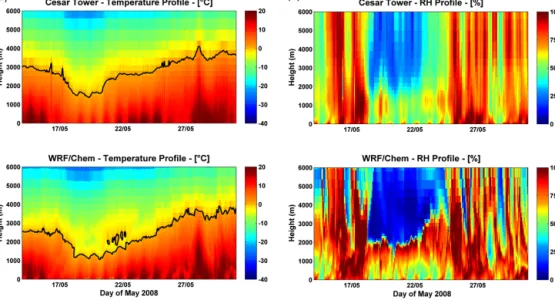
Figure 2 shows the observed and modelled time series of hourly vertical profiles of temperature and relative humid-ity at the Cabauw supersite. WRF-Chem reproduces the day-to-day variation of temperature, before, after, and during the wet period. As shown by statistical indices (Table 2), within the first 200 m, the model reproduces the temperature with a correlation of 0.93–0.95 and a mean bias of about −0.5◦C.
Looking at the free troposphere, we may realize that the model underestimates the height of the 0◦C isotherm (the black line on Fig. 2a) in the first days of simulation and during the wet period by about 200–300 m (i.e., the model is colder than observed by 1–1.5◦C). Whereas immediately after the passage of the cold front, the temperature rise in the simulation is slower than the observed one. The model performances in simulating surface temperature are
consis-Table 2. Statistical indices of the comparison of WRF-Chem to ob-servations of temperature (T ), relative humidity (RH), wind speed (WS), wind direction (WD), ozone (O3), nitrogen oxide (NOx),
ni-tric dioxide (NO2), nitric oxide (NO), ammonia (NH3), nitric acid (HNO3), nitrous acid (HONO), sulfur dioxide (SO2), particle sul-fate (SO4), particle nitrate (NO3), particle (ammonium), and parti-cle OM, collected at Cabauw tower.
Variable R MB NMB NMGE T (◦C) at 2 m 0.93 −0.66 −5.46 10.65 T (◦C) at 10 m 0.93 −0.67 −5.24 9.31 T (◦C) at 20 m 0.94 −0.56 −4.15 8.16 T (◦C) at 40 m 0.94 −0.46 −3.24 7.21 T (◦C) at 80 m 0.95 −0.32 −2.10 5.97 T (◦C) at 140 m 0.95 −0.26 −1.51 5.92 T (◦C) at 200 m 0.95 −0.45 −2.79 6.66 RH (%) at 2 m 0.87 3.17 6.42 11.23 RH (%) at 10 m 0.89 4.44 8.36 11.48 RH (%) at 20 m 0.91 3.04 6.33 10.50 RH (%) at 40 m 0.92 2.99 6.40 10.51 RH (%) at 80 m 0.73 −1.04 2.13 13.34 RH (%) at 140 m 0.92 2.81 6.40 11.19 RH (%) at 200 m 0.91 2.99 7.44 12.50 WS (m s−1) at 10 m 0.78 0.67 27.90 35.56 WS (m s−1) at 20 m 0.66 1.27 40.89 49.32 WS (m s−1) at 40 m 0.67 1.26 32.64 42.04 WS (m s−1) at 60 m 0.72 1.23 24.42 38.99 WS (m s−1) at 140 m 0.74 1.21 28.66 41.55 WS (m s−1) at 200 m 0.76 1.13 27.79 41.48 WD (◦) at 10 m 0.52 27.32 43.31 43.31 WD (◦) at 20 m 0.53 24.80 40.48 40.48 WD (◦) at 40 m 0.60 23.59 40.34 40.34 WD (◦) at 80 m 0.67 20.22 30.34 30.34 WD (◦) at 140 m 0.71 19.21 32.01 32.01 WS (◦) at 200 m 0.73 17.18 28.46 28.46 O3(µg m−3) 0.72 −3.43 70.03 90.88 NOx(µg m−3) 0.70 0.43 19.76 44.77 NO (µg m−3) 0.65 0.28 116.08 167.59 NO2(µg m−3) 0.66 1.25 28.68 54.20 NH3(µg m−3) 0.43 −4.75 −27.72 42.94 HNO3(µg m−3) 0.21 −0.09 −1.22 108.65 HONO (µg m−3) 0.05 −0.56 −95.37 95.37 SO2(µg m−3) 0.48 0.68 90.20 116.33 SO4(µg m−3) 0.56 1.04 92.2 95.4 NO3(µg m−3) 0.68 1.00 72.4 94.3 NH4(µg m−3) 0.74 0.66 63.0 67.3 OM (µg m−3) 0.75 −0.42 3.21 29.9
tent with other European studies (e.g., Zhang et al., 2013a; Brunner et al., 2015). For example, Brunner et al. (2015) compared several meteorology–chemistry coupled models with annual simulations at continental scale, and found that on central Europe the predicted surface temperature shows a correlation with observations in the range of 0.95–0.98, whereas the bias ranges from −1 to 0.1◦C.
Figure 2. Observed and simulated time series of vertical profile of the temperature (a) and relative humidity (b), observed at Cesar observa-tory. The black line on the temperature profile represents the 0◦C isotherm.
The model reproduces the vertical structure of relative hu-midity (Fig. 2b) over the whole period, but it has the ten-dency to overestimate (underestimate) the higher (lower) ob-served values. This behaviour is more evident during scav-enging days, when the relative humidity between 1000 and 2000 m is overestimated on average by 40 %, but sometimes up to 60 %. Errors of this magnitude in simulating the vertical profile of RH were already found in previous works (Mise-nis and Zhang, 2011; Luo and Yu, 2011). Nevertheless, the model correlation and mean bias are 0.84 and +3.4 % below 1000 m of altitude, 0.50 and +13 % in the range of 1000– 2000 m, and 0.78 and +6.4 % between 2000 and 3000 m. These values are comparable with those found by Fast et al. (2014) in the comparison of WRF-Chem simulations to aircraft data. They have shown correlations in the interval of 0.49–0.70, while the bias is from −7 to +0.1 %. Near the surface, the relative humidity is simulated with a correlation of 0.87–0.92 and a positive MB of 3–4 % (+6–8 %).
The biases of the temperature and relative humidity could be due to a misrepresentation of soil (and sea) tempera-ture and soil moistempera-ture or by misrepresentation of the clouds and rain. These two problems are tightly coupled via land surface–atmosphere interaction. The errors in the simula-tion of surface moisture and energy budget influences the fluxes of latent heat and moisture in the atmosphere, af-fecting the local circulation, convective available potential energy (CAPE), cloud formation, and rain pattern (Pielke, 2001; Holt et al., 2006). Moreover, WRF-Chem tends to fail simulating the thermodynamic variables near coastlines, be-cause the uncertainties of land use data may play an impor-tant role (Misenis and Zhang, 2010). Initial and boundary meteorological conditions may also play an important role. Bao et al. (2005) demonstrated that meteorological
predic-tion is sensitive to used input data. They showed that vary-ing the inputs used as initial and boundary conditions, the mean daily model bias ranges from −2.71 to −0.65 K for the temperature and from −0.81 to 0.50 g kg−1for vapour water content.
In Fig. 3 we compare the time series of observed and pre-dicted wind speed and direction at several heights of Cabauw tower. WRF-Chem captures the diurnal trend of wind speed, but it overestimates the wind speed during the night. Gener-ally, we found the higher correlation at 10 and 200 m (0.78 and 0.76 respectively) and higher NMB between 20 and 40 m (+30–40 %). The wind direction is captured at all altitude levels of Cabauw tower, except on 18 May when WRF-Chem does not reproduce some rapid variations most likely due to local effects. The simulation of wind direction tends to improve with height. Indeed, the correlation coefficient in-creases from 0.52 to 0.73 at 10 and 200 m, respectively, and the MB decreases from 27◦below 40 m to 17◦at 200 m. The performance in simulating the surface wind speed are con-sistent with those reported by Brunner et al. (2015) in central Europe. They have shown a correlation for 10 m wind speed in the range of 0.53–0.73 and a mean bias of 1–1.8 m s−1. It is well recognized that WRF tends to overestimate the wind near the surface (e.g. Misenis and Zhang, 2010; Ngan et al., 2013; Brunner et al., 2015), but the bias of the simu-lated wind speed could be also explained with uncertainties in the large-scale pattern of analysis used as input. Bao et al. (2005) showed that varying the meteorological inputs, the mean daily model bias may range from −1.53 to −0.28 and from −1.43 to 0.01 m s−1for the u and v component of the wind, respectively.
Figure 3. Observed (black lines) at Cesar tower and simulated (red lines) time series of wind speed (a) and wind direction (b) at different heights.
4.2 Surface gas phase and aerosol mass
Figure 4 displays the comparison between the observed and modelled hourly time series and average diurnal cycles of O3, NOx, NO2, NO, NH3, HNO3, HONO, and SO2near the surface.
WRF-Chem reproduces the day to day variations of O3, capturing its decrease during scavenging period due to low photolysis rate caused by cloud presence, recovery in the fol-lowing days, and a new decrease starting from 25 May. The average daily cycle is well reproduced with a morning mini-mum and an underestimated maximini-mum in the afternoon. The model simulates the O3 with a correlation of 0.72 and sys-tematic negative bias on average about 3.4 µg m−3. This bias is observed in the afternoon and the evening, and is most likely due to the titration in these hours caused by higher NOxconcentration than observed.
WRF-Chem simulates the NOx, NO, and NO2 time se-ries with a correlation of 0.70, 0.65, and 0.66, respectively. The timing of NOx daily cycle is reproduced. Indeed, the
model captures the morning and evening peaks as well as the diurnal minimum of NO2. The mean bias of modelled NO2is +1.25 µg m−3(+20 %) and occurs in the afternoon and evening hours. Moreover, WRF-Chem reproduces the morning peak and diurnal decrease of NO, but the daily cy-cle is affected by an average positive bias of 0.28 µg m−3, with the average morning maximum overestimation of about 2 µg m−3(+33 %).
Ammonia is reproduced with a correlation of 0.43. WRF-Chem underestimates the NH3 during the scavenging days and from 28 to 31 May. The model captures the daily cycle shape of NH3 concentration average, but the mod-elled NH3concentrations are constantly underestimated. The negative mean bias over the whole period is on average about −4.75 µg m−3 (−28 %). WRF-Chem reproduces the observed HNO3with a poor correlation. The measured mean
diurnal cycle is flat; conversely, the model predicts a noc-turnal minimum and diurnal maximum. The origin of model bias in simulating NH3 and HNO3 is discussed below, to-gether with a discussion on inorganic aerosols.
The nitrous acid concentrations are not well captured by the model and are underestimated by 95 %. This bias could be partly explained by the inefficiency of NO oxidation, the only important reaction known to form HONO. Li et al. (2014), indeed, demonstrated that the major sources of HONO are some unknown reactions that consume nitrogen oxides and hydrogen oxide radicals.
The model reproduces the measured SO2 with a correla-tion of 0.48 and a positive bias of 0.68 µg m−3(+90 %). The overprediction is most likely attributable to anthropogenic emissions. SO2is emitted mainly from isolated and elevated large-point sources (Fig. S1 in the Supplement) that are im-mediately mixed in the model cell leading to overestimation outside of the local plume (Stern et al., 2008). This is demon-strated, for example, by the larger NMGE for SO2than NOx
(116 and 45 %, respectively). NOx is emitted near the
sur-face by traffic and domestic heating. Therefore, NOx
emis-sions are subjected to a stronger temporal modulation than SO2point sources.
The different uncertainties found for the involved species may depend on the choice of the chemical mechanism. Knote et al. (2015a) compared several chemical mechanisms within a box model constrained by the same meteorological con-ditions and emissions, and found that the prediction of the O3 diurnal cycle differs by less than 5 % among the dif-ferent mechanisms. Larger differences were found for other species. For example, the key radicals exhibit differences up to 40 % for OH, 25 % for H2O2, and 100 % for NO3among the selected mechanisms.
Figure 5 shows the simulated and observed time series and diurnal cycle of aerosol sulfate, nitrate, ammonium, and or-ganic matter, at CESAR observatory. WRF-Chem simulates
Figure 4. Observed and simulated time series of gas-phase species (a) and their average diurnal cycle (b), at Cabauw Zijdeweg EMEP station (NL0011R).
the measured SO4, NO3, and NH4with a correlation of 0.56, 0.68, and 0.66, respectively.
WRF-Chem captures the daily variations of SO4 and its decrease during scavenging days. The shape of the diur-nal cycle is also reproduced, with the night-time minimum and diurnal maximum. The mass concentration of SO4 is overpredicted for the whole period with a mean bias of 1.04 µg m−3 (+90 %). The modelled SO4overestimation is directly attributable to SO2 concentration overprediction. Another potential source of the surplus of simulated SO4 is related to an excessive production within the clouds. In-deed, during scavenging days, the particulate sulfate is over-estimated, while the predicted SO2does not show a bias in respect to the measurements. The overestimation of SO4, moreover, explains in part the negative bias of predicted NH3. The excess of particle sulfate consumes too much am-monia (Meng et al., 1997).
NO3 is reproduced with a positive bias of 1 µg m−3 (+72 %). Looking at diurnal cycle, the modelled nitrate is on average biased high in the daytime, with a peak in the af-ternoon. This maximum appears to be correlated with HNO3 maximum. Really, the HNO3peak is caused by evaporation of particulate nitrate formed in the upper PBL (where the conditions of lower temperature and higher relative humidity are favourable to NO3formation), and mixed towards the sur-face by vertical mixing (Curci et al., 2015a; Aan de Brugh et al., 2012). Therefore, the unrealistic afternoon peak of mod-elled nitric acid should result from a too rapid relaxation of aerosol–gas partitioning to thermodynamic equilibrium (Aan de Brugh et al., 2012).
The behaviour of the simulated NH4is related to a mod-elled trend of NO3. It is biased high by 0.66 µg m−3(+66 %). The NH4overestimation is related to NH3underprediction (Meng et al., 1997).
Similar performances are found in reproducing inorganic aerosols at other Dutch EMEP sites (see Sect. 3.1). Daily SO4is simulated with an average correlation (3 stations) of 0.66 and a positive bias of 35 %. WRF-Chem simulates NH4 with a correlation of 0.82 (4 stations) and a bias of +43 %. Predicted daily NO3(measured at only one station) is over-estimated by 15 %.
Organic matter is reproduced with a correlation coefficient of 0.75. WRF-Chem reproduces the right concentration dur-ing the dry period (the decrease in the wet days) and follow-ing recovery. The mean bias is negative by about 0.4 µg m−3 and it is attributable to days from 23 to 26 May. The discus-sion about the origins of OM bias is given in Sect. 4.3, where we will discuss the model evaluation with aircraft data.
The reader should consider that aerosol composition mea-surements performed with the AMS are representative of particles with a diameter between roughly 100 and 700 nm, whereas the model is evaluated with aerosol concentration representative of PM2.5. Therefore, a bias could be present in the comparison. This means that the bias found for in-organic aerosols could be smaller than that reported above; conversely, the OM bias could be larger than that found.
The model evaluation performed so far is representative of few points in the domain and does not include other aerosol components like black carbon or primary PM. This could limit our understanding of the model behaviour. In
or-Figure 5. As in Fig. 4, but for aerosol mass speciation at Cesar observatory observed at 60 m height.
der to overcome this shortcoming, WRF-Chem is also com-pared to daily PM10measurements of the AIRBASE network (Fig. S2). The model captures the daily variations of PM10, the PM10 decrease during scavenging days, the consequent recovery to reach back the background PM10 concentration, and the PM10 enhancement during the long-range transport period. Indeed, the correlations are of 0.72, 0.73, and 0.75 in rural, suburban, and urban zones, respectively. Model bias at rural stations is important in the last days of May 2008; indeed, in these days (28–30 May) it is about −15 µg m−3 (−30 %). Conversely, at suburban and urban stations, the model presents a bias for the most part of the days of about 3–4 µg m−3 (5–10 %) that could partly be explained by the missing source of resuspension due to traffic.
The results obtained here are statistically consistent with other modelling studies over Europe (e.g., Lecœur and Signeur, 2013; Zhang et al., 2013b; Balzarini et al., 2015). For example, the results of European annual simulations of Balzarini et al. (2015) exhibited a correlation of 0.48, 0.60, and 0.56 for surface SO4, NO3, and NH4, respectively. Dur-ing EUCAARI campaign, Athanasopoulou et al. (2013) re-ported a mean correlation of surface OM with observations of 0.56 and a mean bias of −0.5 µg m−3, whereas Fountoukis et al. (2014) simulated the OM at Cabauw on May 2008 with a bias of 0.3 µg m−3. Moreover, with regards to surface PM10, our performances are comparable to those found, for example, by Im et al. (2015) over Europe with annual
sim-ulations in terms of correlation, but are higher in terms of bias. Comparing PM10concentrations from several models, Im et al. (2015) found correlations of 0.18–0.86 and 0.07– 0.82, and bias of about −40 and −50 % for rural and urban sites, respectively. This improvement is most likely due to the very high resolution used in this study with respect to the 23 km of Im et al. (2015), since the anthropogenic emissions inventory used is the same here and in the study by Im et al. (2015).
4.3 Aloft aerosol mass concentration
The comparison of WRF-Chem to aircraft data is done by interpolating the model output point by point along the flight track. Observed and modelled aircraft data are presented by using the box plots for planetary boundary layer (PBL) and free troposphere (FT) (see Fig. 6). The height of the PBL was lower than 1600 m during the whole campaign (Crumeyrolle et al., 2013). Therefore, we considered for PBL and FT concentrations the data below and above 1600 m up to 3000–4000 m, respectively. This rough approximation of PBL height could affect the comparison of the model to data. Figure 6 displays the observed and modelled box plots of the mass concentration of SO4, NO3, NH4, and OM for PBL and FT. Their mean value, standard deviation, relative mass fraction, and correlation coefficients, averaged over the whole period of interest, are reported in Table 3.
SO4(µg m−3) 3.1 ± 2.4 (19 %) 3.2 ± 2.1 (24 %) 0.39 2.6 ± 2.0 (29 %) 2.5 ± 1.2 (38 %) 0.23 NO3(µg m−3) 4.5 ± 5.4 (28 %) 4.6 ± 5.1 (34 %) 0.47 1.3 ± 3.0 (14 %) 1.5 ± 2.7 (23 %) 0.44 NH4(µg m−3) 2.6 ± 2.2 (16 %) 2.4 ± 2.1 (19 %) 0.43 1.4 ± 1.5 (16 %) 1.2 ± 1.2 (19 %) 0.42 OM (µg m−3) 6.1 ± 5.8 (37 %) 3.0 ± 2.6 (23 %) 0.67 3.7 ± 4.5 (41 %) 1.3 ± 1.4 (20 %) 0.52 PM2.5(µg m−3) 23 ± 13 16 ± 10 0.75 19 ± 17 12 ± 9 0.80 CN (103# cm−3) 6.7 ± 5.0 9.4 ± 5.4 0.40 1.0 ± 1.1 1.7 ± 2.8 0.74 CCN (103# cm−3) 0.6 ± 0.5 0.9 ± 0.8 0.45 0.3 ± 0.3 0.3 ± 0.3 0.73
Figure 6. Box plot of SO4, NO3, NH4, and OM mass concentrations measured by AMS aboard the ATR-42 (blue) and simulated by WRF-Chem (red) within boundary layer (a) and free troposphere (b). The x axis reports the day of May 2008 (black) and the number of the research flight (red). The whisker plots denote median, 25th and 75th percentiles, 1.5 × (inter-quartile range), and outliers. The squares represent the mean values.
The average concentrations of inorganic aerosols show lit-tle absolute error (2–8 %) with respect to the observations in the PBL, while the NO3 and NH4 mean concentration presents a bias of +14 and +20 % (+0.3 and +0.2 µg m−3), respectively, in the FT. The mean OM mass is biased low by a factor of 2 and 3 in the PBL and FT, respectively. The correla-tion coefficients of SO4, NO3, NH4, and OM are 0.39, 0.47, 0.43, 0.67 in the PBL and 0.23, 0.44, 0.42, 0.53 in the FT. These performances are comparable with those found with WRF-Chem (but with a different chemistry package) in Cal-ifornia by Fast et al. (2014). They reported an absolute mean bias of about 0.01–0.2, 0.03–0.6, 0.1–0.45, 0.2–0.57 µg m−3 and a mean correlation of 0.42, 0.45, 0.44, and 0.72 for SO4, NO3, NH4, and OM, respectively.
Although the predicted aerosol mass of each species is within the range of the observed values for most of the flights used in this study (see Fig. 4), the model does not capture the full range of the measured concentrations. This assertion is made quantitative by the standard deviations reported in Ta-ble 3. The predicted standard deviations for each species are lower than observed. In the PBL, the observed and modelled standard deviations differ by 4–10 % for inorganic ions and 55 % for OM. In the FT, the differences are higher than in the PBL. The model predicts standard deviations lower than 10– 40 % for inorganic particles and lower than 65 % for organic matter with respect to the measurements.
For the purpose of this analysis, it is also interesting to explore how the model reproduces the relative fraction of
aerosol mass species with altitude (see Table 3). WRF-Chem overpredicts the relative fraction of the SO4and NO3by few percent in the PBL and about 10 % in FT, while the relative mass of NH4is overestimated by 3 % along the whole pro-file. The relative amount of OM is underpredicted by about 20 % in both PBL and FT. The decrease of relative amount of NO3and increase of SO4with altitude is captured by the model. The modelled relative mass of NH4and OM is near constant with altitude as well as in the observations.
Looking at the individual flights, it is possible to note how the model captures the aerosol mass trend as a function of the synoptic frame in both the PBL and FT, during the dry period, scavenging days, and dust period characterized by southerly wind and passage of several fronts. The FT is a layer mainly affected by long-range transport and cloud con-tamination. Therefore, the relative small bias in simulating aerosol inorganic mass in FT means that the model resolves quite correctly the large-scale transport and processes related to clouds.
Nevertheless, it should be noted that SO4is overestimated for 8 out of 14 RFs, while NO3and NH4are underpredicted for 7–8 out of 14 RF. This SO4overprediction is attributable to the SO2excess and to a potential overproduction within the cloud chemistry scheme. The negative bias of NO3and NH4could be explained by a low NH3regime, that limits the formation of the ammonium–nitrate.
The simulated OM concentration is always at the lower end of the observed variability. Several factors may explain this systematic bias. First of all, our simulations do not in-clude the processing of organic compounds in aqueous chem-istry. SOA may be produced in the clouds (Hallquist et al., 2009). Modelling studies suggest that the contribution of cloud chemistry to SOA budget is almost as much as the mass formed from the gas phase (Ervens et al., 2011). OM prediction is also affected by meteorological errors. Bei et al. (2012) found that the uncertainties in meteorological ini-tial conditions have a significant impact on the simulations of the peaks, horizontal distribution, and temporal variation of SOA. The same authors demonstrated that the spread of the simulated peaks can reach up to 4.0 µg m−3. Other uncertain-ties may be related to the VBS formulation. The SOA forma-tion pathway is one these, indeed halving the SOA yields the concentration of SOA decreases by 30 % (Ahmadov et al., 2012). Moreover, the assumption on the deposition velocity of the OCVs may play an important role in the uncertainties of SOA production. The OCV deposition velocity in the ver-sion of the VBS implemented in WRF-Chem by Ahmadov et al. (2012) is proportional to the deposition velocity of the HNO3. The proportionality constant is a tunable parameter and in this work is set to the default value of 0.25. WRF-Chem prediction of SOA mass is very sensitive to the choice of the proportionality constant (Ahmadov et al., 2012). Pre-vious studies have shown that SOA concentration is highly sensitive to the treatment of the deposition velocity of OCVs (Bessagnet et al., 2010; Knote et al., 2015b). Finally, we note
Figure 7. Same as Fig. 6 but for observed and simulated PM2.5 mass concentrations. The blue colour represents the observations, while the model is displayed in red colour.
that OM bias could be partially explained by the uncertainties in the anthropogenic emissions (e.g. bias or spatial distribu-tion) of primary organic carbon and in the factor 1.6 used to convert them to POM (Turpin and Lim, 2001). The reader should also consider that the uncertainties in POM simula-tion affect the SOA formasimula-tion. Indeed, the partisimula-tion between OCV and SOA used in the VBS approach depends on the total OM (Eq. 1 of Ahmadov et al., 2012); thus, if POM is underpredicted the resulting SOA could be underestimated.
In order to have a more complete overview of the model skill in reproducing the upper air aerosol mass concentration, we also compare the observed and modelled PM2.5. Figure 7 shows measured and predicted box plots of the PM2.5 con-centration in PBL and FT. Modelled PM2.5 is in the range of the observed values within the PBL expect during the wet scavenging period when it is at the lower end of the observa-tions. In FT, conversely, predicted PM2.5 is at the lower end of the observed profiles for the most part of the flights. The comparison between modelled and observed PM2.5 concen-tration within PBL and FT show good correlations (0.75 and 0.80, respectively).
Model correlation with observations is high, 0.75 and 0.80 in PBL and FT, respectively. The absolute mean bias is
−7 µg m−3(30–35 %) in both PBL and FT.
Although the box plot and statistical summary (Table 3) provide significant information on the model performances, the model skills in reproducing vertical profiles of aerosol properties need to be evaluated. Therefore, we also look at model vertical profiles along the flight tracks. As an exam-ple, we have chosen the 14 May 2008 (RF50) for two rea-sons: first, there is a relatively large contribution of OM, SOA (70–85 % of OM), and CCN (see Fig. 10), and second, it is a day of high pressure; thus, the interpretation of the
re-Figure 8. Vertical profiles (shadow) along the flight track of 14 May (RF50) of modelled PM2.5(a), SO4(b), NO3(c), NH4(d), and OM (e). The circles are the measurements collected aboard the ATR42.
sults is not complicated by cloud processes. Figure 8 displays the comparison of modelled vertical profiles of PM2.5, SO4, NO3, NH4, and OM along the flight track and measurements. WRF-Chem captures several features present in the aircraft observations. Both observed and modelled PM2.5 exhibit a maximum in a layer between 500 and about 2000 m. The model predicts the inhomogeneity of the chemical secondary species of PM2.5 also displayed in the observations: SO4 and OM concentrations are relatively homogeneous within the PBL, whereas NO3and NH4show enhanced concentra-tions in the upper levels of the PBL. For completeness, we note that primary PM2.5 components (not shown) have their maximum close to the surface (first 500 m) and are diluted throughout the PBL. These results are qualitatively similar to those found by Curci et al. (2015a) above Milan (Italy).
4.4 Aloft aerosol particles
The comparison of WRF-Chem output with aircraft measure-ments of the number concentration of condensation nuclei (CN) and of CCN at 0.2 % of supersaturation is done by us-ing the box plots as for aerosol mass. In this case the mod-elled and measured data are smoothed by using a 10 s running mean.
Figure 9 reports the comparison of observed and modelled CN within PBL and FT. The measured and predicted average, standard deviation, and correlation of the CN number over the whole period of our analysis are reported in Table 3.
The model resolves the decrease of a factor of 5–6 of CN concentration between the PBL and the FT. The differences
Figure 9. Same as Fig. 6 but for observed and simulated conden-sation nuclei (CN) concentrations. The blue colour represents the observations while the model is displayed in red colour.
in simulated concentrations between land and sea (RF51 and 52) are also captured by the modelling system. Nevertheless, WRF-Chem overestimates, on average, the observed CN by a factor of 1.4 within PBL and 1.7 within the FT. The bias is less pronounced above the sea during the RF51 and RF52, where the anthropogenic sources are less important. More-over, it should be noted that in some cases, for example dur-ing the RF56, 57, and 58, the predicted CN are completely
Figure 10. Same as Fig. 6 but for observed and simulated cloud con-densation nuclei (CCN) concentrations at 0.2 % of supersaturation. The blue colour represents the observations, the model is displayed in red colour.
outside the range of the observed values. In these cases the predicted CN are biased high by about a factor of 2–3. Pre-dicted CN concentration shows a higher variability than mea-sured, especially in the free troposphere where the difference of modelled standard deviation is biased high by 155 %. Any-way, the modelled CN concentration correlates well with the observed one (0.40 and 0.74 in PBL and FT, respectively). These values are consistent with the 0.61 found by Luo and Yu (2011) studying the new particle formation and its con-tribution to CN with a version of WRF-Chem including an advanced aerosol microphysical model.
Figure 10 shows the comparison of observed and mod-elled CCN at 0.2 % of supersaturation. The measured and predicted average and standard deviation of CCN are showed in Table 3. The bias of simulated CCN0.2appears more con-tained with respect to CN prediction, especially in the free troposphere. Figure S3 shows the comparison of the mod-elled vertical profile of CCN along the flight track of 14 May and observed CCN aboard the ATR42. WRF-Chem predicts relatively homogeneous profile of CCN in the PBL also shown by observations.
The aerosol particles that mostly contribute to the CCN number are those of accumulation and coarse modes, and accumulation and coarse-mode particles are also the major contributor to PM2.5mass concentrations. Since PM2.5is un-derestimated and CCN overestimated, CCN bias cannot de-pend on model errors in PM2.5. The major uncertainties in predicted CCN arise from aerosol nucleation rate and pri-mary emissions (Lee et al., 2013). Direct emission of aerosol particles is the key factor for CCN production in the PBL and near particle sources (Spracklen et al., 2006), and ac-count for 55 % of the total global production (Merikanto
et al., 2009). On the other hand, nucleation and subsequent growth up to CCN size is an important mechanism of CCN formation in many parts of the atmosphere (Sotiropoulou et al., 2006). Using several nucleation parameterizations, Pierce and Adams (2009) showed that CCN on average varies by up to 12 % within the PBL. At the same time, they also found that varying by a factor of 3 the primary emissions, the CCN mean changes by 40 % in the PBL. On the basis of these ar-gumentations and the correlation between predicted and ob-served CN being larger in the FT than in PBL (i.e. far from anthropogenic sources), we may speculate that the errors in the CCN prediction arise mainly from the uncertainties in the primary emissions of the aerosol particles and in their distri-bution in the log-normal modes.
The analysis of CCN efficiency reveals other interesting features in the model behaviour. The CCN efficiency is given by the CCN / CN ratio and represents the ability of aerosol particles to nucleate cloud droplets (Andreae and Rosenfeld, 2008). CCN efficiency observed during the studied RFs is in the range of 0.02–0.33 for PBL and 0.18–0.41 in the FT, while the model predicts values of 0.03–0.17 and 0.04–0.18 for PBL and FT, respectively. In other words, WRF-Chem underestimates the CCN efficiency by a factor of 1.5 and 3.8 within the PBL and FT, respectively. Moreover, the modelled CCN efficiency, contrary to the observation, shows almost the same range of values within the PBL and within the FT.
The so-calculated and modelled CCN efficiencies could be underestimated. In general, the CCN efficiency should be computed with the aerosol population with size larger than the minimum activation diameter (Asmi et al., 2012). The latter depends on the aerosol type and ranges from about 50 to 125 nm. We calculated the observed CCN / CN ratio with the measurements of CPC 3010 which gives the total num-ber of particles larger than 15 nm, and the modelled CCN fraction is calculated with total particle number given by the sum of the three modes of the log-normal distribution (Aitken, accumulation and coarse). In order to better charac-terize the relationship between CCN and the corresponding aerosol population in the model, predicted CCN efficiency was also calculated with particles of the accumulation and coarse modes (the most favoured particles to act as CCN), and it was qualitatively compared to observed efficiency dur-ing the IMPACT campaign computed with particles larger than 100 nm. Observed values of CCN efficiency are in the range of 0.28–0.4 and 0.38–0.6 in the PBL and FT (Crumey-rolle et al., 2013), respectively. The simulated CCN fraction calculated with the particles of the accumulation and coarse modes, is always underestimated with respect to the observa-tions, and it is in the range of 0.17–0.3 in PBL and 0.23–0.36 in FT. The model deficiency in simulating the CCN / CN ra-tio could be attributable to the uncertainties in geometrical diameter and bulk hygroscopicity of the log-normal modes, and updraft velocity that lead to error in the prediction of minimum activation diameter of each mode.
Figure 11. Aerosol optical thickness at 500 nm from MODIS-Aqua (a) and WRF-Chem simulations (b) on 14 May 2008.
4.5 Comparison with MODIS data
WRF-Chem output was also compared to AOT, cloud micro-physical, and optical properties retrieved by MODIS-Aqua.
Figure 11 shows the comparison between the AOT at 550 nm measured by MODIS and the corresponding AOT predicted by the model during the high-pressure period on 14 May 2008. WRF-Chem reproduces the spatial distribu-tion of observed AOT, such as the lowest values in the south-ern part of the domain or the highest values around Cabauw, but underestimates the strong gradient between the eastern boundary and the centre of the domain. The model over-estimates the regional mean of AOT; indeed, the domain averages are 0.38 ± 0.12 and 0.42 ± 0.10 for MODIS and WRF-Chem data, respectively. Unfortunately, good cover-age of the D3 domain by MODIS was achieved only on 1 day (14 May 2008), this does not allow us to have a gen-eral overview of model skill in predicting AOT. In gengen-eral, model intercomparisons revealed that a large part of the un-certainties in simulating the AOT arises from the assumption on the mixing state. For example, AOT computed with ex-ternal mixing is larger by 30–35 % of that calculated with internal mixing assumption (Curci et al., 2015b). For typi-cal atmospheric particle sizes and in the visible wavelength range, the AOT is then expected to be lower under inter-nal mixing assumption (that is the assumption done in this work). Moreover, a 10 % error in predicting AOT may be at-tributable to the choice of species density, refractive index, and hygroscopic growth factor (Curci et al., 2015b).
As the WRF microphysics scheme accounts for aerosols only within liquid clouds, comparison among predicted cloud optical and microphysical properties with MODIS data was done separately for liquid, excluding mixed clouds. Top liquid cloud Re was calculated from liquid water content (LWC) and cloud droplet number concentration predicted by WRF-Chem. Liquid water path (LWP) was calculated by ver-tically integrating liquid cloud mixing ratios (water and rain water), while liquid COT was estimated from LWC and Re. Since MODIS L2 data provide the total cloud water path
(CWP), combined effective radius for all cloud types and total (water and ice) COT, the observed contribution to the liquid water cloud was separated by using the retrieved top cloud phase, i.e. were discarded mixed clouds.
The comparison between the predicted and observed Re, LWP, and liquid COT was done in the scavenging back-ground and long-range transport periods in the days when MODIS cloudy pixel coverage was larger than 60 %. Fig-ure 12 shows the comparison of the averaged values for 17– 19 May 2008 period (1P). The same comparison has been done on averaged values for 25–27 (2P) and 28–30 May (3P) and are reported in the Supplement (Figs. S4 and S5). WRF-Chem reproduces several features of the liquid cloud systems during 1P: the liquid cloud distribution, the maxi-mum values of Reclose to the coast, maximum of LWP, and liquid COT on the centre and at north-east of the domain. However, model results present a larger spatial extension of liquid water cloud highest values off the Dutch and Belgian coasts not observed in the MODIS data. During 2P the struc-ture of the cloud system is not completely reproduced by the model. Although Re value magnitude is captured above the sea, WRF-Chem underestimates the cloud droplet dimension on the land. Therefore, LWP and liquid COT structure on the sea is resolved by the model, whereas on the land they are too small compared to the observations. Finally, the model reproduces the average structure of the cloud system in 3P, but LWP and liquid COT are overestimated on the western part of the domain.
As shown in Table 4, Re values averaged over the entire domain are underestimated by the model by a factor of about 1.5 during all three periods of interest. LWP, values averaged over the entire domain, is also overestimated in all three cases by a factor of 1.1, 1.3, and 1.6 for 1P, 2P, and 3P, respectively. The Re(LWP) underprediction (overestimation) may be due to the overestimation of droplet number concentration that stems from overestimation of CN. Another reason that could explain the positive bias of modelled LWP is the inefficient autoconversion of cloud water to rain, typical of the Morrison microphysical scheme (Saide et al., 2012). The consequence
Figure 12. The 17–19 May 2008 averages of droplet effective radius at cloud top (first row), liquid water path (second row), and liquid cloud optical thickness (third row), retrieved using MODIS-aqua observations (first column), predicted by model in the references run (CTRL, second columns) and sensitivity test without SOA (NOSOA, third column).
of the negative (positive) of Re(LWP) is the overestimation of average liquid COT by few percent for 1P and 3P, and 42 % for 3P.
The biases found here are quite different from the WRF-Chem study by Yang et al. (2011) on the modelling of marine stratocumulus in the south-east Pacific. They have shown a bias of +30 % in reproducing the COT, while LWP was un-derestimated by a factor of 1.3. The reader should note that in Yang et al. (2011), the aerosol model adopted was different from the one used here and SOA formation was not included at all.
Figure 13 displays the distribution functions (DF) of Re, LWP, and liquid COT for 1P. The DF for 2P and 3P are reported in the Supplement (Figs. S6 and S7). In all three periods analysed, the model captures the frequency of large droplets (Re>18–20 µm), underestimates the number of small droplets (8–10 < Re<18–20 µm), and overestimates the frequency of very small cloud droplets (Re<8–10 µm) by more 30 %. Whereas DF of the observed Represents the maximum in the range of 8–13 µm, modelled DF shows the maximum values in correspondence of the droplets with size less than 7–8 µm. WRF-Chem captures the shape of the dis-tribution functions of LWP and liquid COT, but underesti-mates the maximum and overestiunderesti-mates the higher and lower
end of the distributions. Both variables show a variability higher than the observations. The predicted standard devi-ations (Table 4) are about 2–3 and 1.5 times larger than those observed for LWP and liquid COT, respectively. This proba-bly stems from the large variability in simulated CCN.
Now it is interesting to analyse the model behaviour in reproducing the total CWP and COT given by contribution of all cloud phases. Modelled CWP was calculated by ver-tically integrating all cloud mixing ratios (water, rainwater, ice, snow, and graupel). Predicted COT is given by the con-tribution of the liquid water and ice. The concon-tribution of the liquid water was calculated as described above for liquid wa-ter cloud. The contribution of ice phase to COT was calcu-lated following Ebert and Curry (1992).
Figure 14 displays the comparison between observed and predicted CWP and COT in P1, whereas the same figures for P2 and P3 are reported in the Supplement (Figs. S8 and S9). Although for all three cases, the model reproduces with good approximation the shape and localizations of the cloud sys-tems, CWP and COT are systematically overestimated (ex-cept COT in P2). As shown in Table 5, the predicted domain average of CWP presents, indeed, a bias of 62, 41, and 80 % for P1, P2, and P3, respectively, whereas the bias of COT is about 15 % in P1 and P3.
17–19 May 10.2 ± 3.5 7.5 ± 3.5 8.5 ± 4.3 230 ± 343 242 ± 343 208 ± 352 32 ± 22 33 ± 33 21 ± 24 25–27 May 13.7 ± 3.7 9.1 ± 4.4 9.8 ± 4.9 200 ± 166 256 ± 502 273 ± 480 22 ± 19 23 ± 30 21 ± 27 28–30 May 10.7 ± 3.9 8.4 ± 4.1 7.8 ± 3.6 141 ± 128 224 ± 327 243 ± 447 19 ± 14 27 ± 27 24 ± 30
Figure 13. The 17–19 May 2008 averages of observed and simulated distribution function of droplet effective radius at cloud top (a), liquid water path (b), and liquid cloud optical thickness (c). The black line represents the observations retrieved by MODIS, blue and red colours correspond to model predictions from the reference run (CTRL) and sensitivity test without SOA (NOSOA), respectively.
At this point of the analysis, although the aerosol–cloud interaction is a very complex non-linear process, we are able to relate the model error in aerosol particles to the uncertain-ties in cloud prediction. The overestimation of CN leads to overprediction of the CCN. Higher number of CCN means clouds with a higher number of cloud droplets, higher water content, smaller droplets, and clouds optically deeper.
In addition to the uncertainties in aerosol particle simula-tion, one typical source of error in the prediction of cloud fields is the choices related to the model setup. For exam-ple Otkin and Greenwald (2008) found a strong sensitivity of cloud properties while evaluating the response of the WRF model to the permutation of several PBL and cloud micro-physical schemes. Moreover, the same authors have shown that the low level clouds are sensitive to PBL parameteriza-tion, whereas the upper level clouds are sensitive to both PBL and microphysics schemes.
One element that may affect the model–satellite compar-ison are the uncertainties associated with the retrieval. For example, in South Pacific stratocumulus, MODIS overesti-mates the droplet effective radius by 13–20 % with respect to concomitant in situ measurements (Painemal and Zuidema, 2011; King et al., 2013). The overestimation of COT by MODIS results in the overestimation of CWP (King et al., 2013). Henrich et al. (2010) have shown systematic differ-ences between MODIS data and in situ observations. Indeed, analysing a system of thin cumulus clouds during the EU-CAARI campaign, they also found that MODIS overesti-mates the droplet effective radius by a factor of 2–3 and COT is 2–3 times lower than the in situ measurements.
Table 5. MODIS and modelled mean values and standard deviations of cloud water path and cloud optical thickness of clouds in all phases, on 17–19, 25–27, and 28–30 May 2008.
CWP (g m−2) COT
MODIS-Aqua CTRL NOSOA MODIS-Aqua CTRL NOSOA 17–19 May 207 ± 203 336 ± 531 218 ± 359 26 ± 20 30 ± 33 19 ± 23 25–27 May 235 ± 182 331 ± 533 244 ± 418 21 ± 16 17 ± 23 16 ± 21 28–30 May 206 ± 201 370 ± 714 262 ± 523 21 ± 16 24 ± 26 21 ± 27
Figure 14. As in Fig. 12, but for clouds in mixed phase.
5 Impact of SOA particles on cloud prediction
The last part of this study focussed on the evaluation of the impact of SOA on the simulation of cloud fields. We per-formed sensitivity simulations during P1, P2, and P3 without the SOA (NOSOA), and compared them to the reference run (CTRL) discussed so far. NOSOA runs are carried out only in the higher resolution domain (D3). The simulations of all three periods are initialized at 00:00 UTC with the same me-teorological and chemical input data used for CTRL, except chemical initial conditions that are restarted by a previous NOSOA run. Each period is preceded by 30 h of simulation used as spin-up for D3 chemistry. The sensitivity simulation is performed zeroing the arrays pertaining to SOA. Thus, the SOA fields are not affected by incoming SOA from do-main boundaries or by local production. We did not perform the sensitivity tests with the SORGAM option because this model produces very little SOA mass concentrations (Grell at al., 2005; McKeen et al., 2007; Tuccella et al., 2012). There-fore, we may assume that simulations with SORGAM and without SOA (in VBS option) are roughly equivalent. The advantage of this assumption is that the model is forced with the same initial meteorological conditions and boundary me-teorological and chemical conditions as the CTRL
simula-tion. The use of SORGAM would require running the model on all three domains, leading to different results on D2 which is used to initialize D3. Finally, this would introduce depen-dencies on the D3 input data making the comparison not di-rectly comparable to the CTRL run.
The comparisons of Re, LWP, and liquid COT simulated in CTRL and NOSOA runs with MODIS data are reported in Figs. 12, S4, and S5. In general, the average spatial pat-tern of these three variables is captured better by the CTRL simulation with respect to the NOSOA run, especially in P1. Figures 13, S6, and S7 display the comparison between DFs of the cloud properties simulated by CTRL and NOSOA runs with those retrieved with the MODIS observations. The domain averages for each variable are reported in Table 4. NOSOA runs show a domain averaged Relarger than CTRL. DFs of the LWP are different between the runs, but it is not clear if there are improvements in CTRL with respect to the NOSOA run. Only the domain averages allow one to estab-lish that LWP values predicted by CTRL run are closer to the observed means than NOSOA. The presence of SOA in the numerical prediction improves the DF of liquid COT with re-spect to NOSOA simulation in P1 and P3, whereas there are no differences during P2. NOSOA has 10 and 3 % more