Multipoint concentration statistics for transport in stratified random velocity fields

HAL Id: insu-00562481

https://hal-insu.archives-ouvertes.fr/insu-00562481

Submitted on 3 Mar 2021

HAL is a multi-disciplinary open access

archive for the deposit and dissemination of

sci-entific research documents, whether they are

pub-lished or not. The documents may come from

teaching and research institutions in France or

abroad, or from public or private research centers.

L’archive ouverte pluridisciplinaire HAL, est

destinée au dépôt et à la diffusion de documents

scientifiques de niveau recherche, publiés ou non,

émanant des établissements d’enseignement et de

recherche français ou étrangers, des laboratoires

publics ou privés.

Multipoint concentration statistics for transport in

stratified random velocity fields

Marco Dentz, Jesus Carrera, Diego Bolster, Tanguy Le Borgne

To cite this version:

Marco Dentz, Jesus Carrera, Diego Bolster, Tanguy Le Borgne. Multipoint concentration statistics

for transport in stratified random velocity fields. Physical Review E : Statistical, Nonlinear, and

Soft Matter Physics, American Physical Society, 2009, 80, pp.036306. �10.1103/PhysRevE.80.036306�.

�insu-00562481�

Multipoint concentration statistics for transport in stratified random velocity fields

Marco Dentz

*

and Jesus Carrera

Institute of Environmental Assessment and Water Research (IDÆA-CSIC), 08034 Barcelona, Spain Diogo Bolster

Department of Geotechnical Engineering and Geosciences, Technical University of Catalonia (UPC), 08034 Barcelona, Spain Tanguy Le Borgne

Géosciences Rennes, UMR 6118, CNRS, Université de Rennes 1, 35042 Rennes, France 共Received 12 May 2009; revised manuscript received 17 July 2009; published 11 September 2009兲 We determine the full multipoint concentration statistics for superdiffusive transport in a steady stratified random velocity field. Using a Lagrangian approach, we derive explicit analytical expressions for the multi-point moments of concentration and specifically for the concentration variance, which is a measure for con-centration uncertainty. The multipoint concon-centration moments are fully characterized by the Lagrangian mean velocity and by the one and two particle velocity correlations. While the relative variance at the center of mass of the mean concentration is constant, it increases exponentially with time and distance from the center of mass. This implies that small concentration values are particularly uncertain, which can pose a serious practical concern as these are typically the earliest and latest to arrive at a point.

DOI:10.1103/PhysRevE.80.036306 PACS number共s兲: 47.60.⫺i, 92.40.Kf, 05.60.⫺k, 05.10.Gg

I. INTRODUCTION

Observed transport behavior in fluctuating environments is often anomalous. That is, the distribution of a transported quantity cannot be described by the classical advection dis-persion equation共e.g., 关1–4兴兲. Even when transport may

fol-low the advection-dispersion equation on a “local” scale, the effective large scale transport in natural environments does not. Spatiotemporal fluctuations can have a dual effect. On one hand, they act on the mean transport behavior and lead to effective transport dynamics that are different from their local scale counterpart. On the other hand, they introduce uncertainty due to limited knowledge on the fluctuation de-tails. Oftentimes the only possible description of the fluctu-ating environment is statistical. Given such a statistical de-scription, the transport behavior can be modeled by a stochastic approach. The latter provides a straightforward framework for both the quantification of the effective, mean transport behavior and the related uncertainty.

A series of applications require the quantification of both heterogeneity induced effective large scale transport and un-certainty. These include the safety assessment of geological hazardous waste facilities共e.g., 关5,6兴兲, groundwater

manage-ment共e.g., 关7,8兴兲 and carbon sequestration in geological

me-dia 共e.g., 关9,10兴兲. Another potential application is the

move-ment of objects on the ocean surface and transport in turbulent and chaotic flows 共e.g., 关11兴兲. Capturing the

influ-ence of heterogeneity can often be achieved by stochastic or spatial averaging over the local scale transport problem. In more general terms, one can perform a dimensional reduc-tion or projecreduc-tion of the local scale processes. Such averag-ing implies a loss of information, which in general leads to a non-Markovianity property of the projected process 共e.g.,

关12兴兲. Furthermore, spatial heterogeneity induces fluctuations

about this mean behavior, which can be quantified by the ensemble variance of the distribution density c共x,t兲, which is defined by

␴c

2_{共x,t兲 = 关c共x,t兲 − c¯共x,t兲兴}2_{, 共1兲} where the overbar denotes the ensemble average, c¯共x,t兲 is

the mean concentration. For transport in heterogeneous po-rous media the concentration variance has been studied in, e.g., Refs.关13–16兴 and is of general interest for transport in

spatially fluctuating flow fields because it gives valuable in-formation on the mixing properties of a passive scalar共e.g., 关11,17,18兴兲. In principle, the complete characterization of the

process requires the knowledge of the full multipoint statis-tics of concentration. The latter have been looked at by using PDF 共probability density functions兲—methods in, e.g., Refs. 关11,19,20兴. Frequently, the analysis of the concentration

vari-ance and the multipoint statistics is limited to perturbation theory and to so-called assumed PDF methods共e.g., 关11,15兴兲.

Here we present a nonperturbative, exact study of the multipoint concentration statistics for transport in a stratified random velocity field. The specific model under consider-ation has been introduced by关21兴 to study dispersion

mecha-nism in heterogeneous porous media. Since then, this model has been subject to intense research共e.g., 关3,22–25兴兲 because

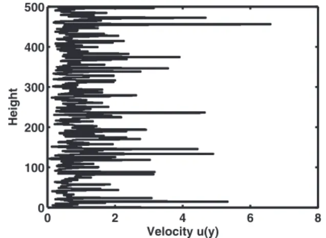
it provides a relatively simple but nontrivial model to study the possible mechanisms that lead to superdiffusive behavior 共i.e., a superlinear growth of the spatial variance兲 in hetero-geneous media in particular and stratified random velocity fields in general. This model can be regarded as an approxi-mation to aquifers characterized by vertical stratification of-ten observed in geological media 关26,27兴. Figure1 shows a realization of the type of velocity fields under consideration in this paper. Previously,关28兴 showed that effective transport

in such a velocity field is non-Markovian and described by a Gaussian concentration distribution. Here we extend this *[email protected]

work and derive explicit expressions for the n-point mo-ments of concentration.

II. MODEL

Transport of a passive scalar g共x,t兩x2

⬘

兲 in a stratified flow field u共x2兲 can be described by the advection diffusion equa-tion ⳵g共x,t兩x₂

⬘

兲 ⳵t = − u共x2兲 ⳵g共x,t兩x₂

⬘

兲 ⳵x₁ + D ⳵2_g共x,t兩x 2

⬘

兲 ⳵x₂2 , 共2兲

where the coordinate vector is given by x =共x1, x2兲T; D is the diffusion coefficient. For simplicity, we restrict this study to an infinite d = 2 dimensional domain with no diffusion in the flow direction. The following analysis can be easily extended to more than two spatial dimensions and longitudinal diffu-sion. The spatial density g共x,t兩x2

⬘

兲 and its gradients at infin-ity are zero. The initial distribution is given by g共x,t = t0兩x2

⬘

兲=␦共x1兲␦共x2− x2

⬘

兲 共which means that g共x,t=t0兩x2

⬘

兲 can be regarded as a Greens function兲. The stratified flow field

u共x2兲 is a realization of a stationary spatial Gaussian random process 兵u共x₂兲其 characterized by the constant ensemble mean velocity uE= E关u共x2兲兴 and correlation of the velocity fluctuations u

⬘

共x2兲=u共x2兲−uE, which is CE共x2− x2

⬘

兲 = E关u

⬘

共x₂兲u

⬘

共x₂

⬘

兲兴. The notation E关·兴 stands for the ensemble average.

We consider now an ensemble of initial plumes that are distributed vertically according to␳共x2兲; ␳共x2兲 is normalized to one, its variance is denoted by a2_{. For aⰇ1, it is assumed} to have the scaling form

␳共x2兲 ⬃ 1

af␳

冉

x2

a

冊

, 共3兲

where f_␳共0兲 is constant. Sampling the ensemble of concen-tration distributions along the vertical and taking the limit of

a→⬁ gives the mean concentration

c ¯共x₁,t兲 = lim a→⬁ 1 a

冕

−⬁ ⬁ dx₂

⬘

f_␳

冉

x2

⬘

a

冊

c共x1,t兩x2

⬘

兲, 共4兲

where we defined the projected concentration

c共x₁,t兩x₂

⬘

兲 ⬅

冕

−⬁

⬁

dx₂g共x,t兩x₂

⬘

兲. 共5兲

The mean squared concentration is defined accordingly by

c2_共x 1,t兲 = lim a_→⬁ 1 a

冕

_−⬁ ⬁ dx₂

⬘

f_␳

冉

x2

⬘

a

冊

c共x1,t兩x2

⬘

兲 2_{. 共6兲}

This averaging procedure is equivalent to performing the ensemble average over the concentration distribution evolv-ing from a point injection because the random shear flow is assumed to be an ergodic random field共recall aⰇ1兲. In the following we derive explicit expressions for the multipoint moments of concentration in general and for the concentra-tion variance␴c

2_共x

1, t兲=c2共x1, t兲−c¯共x1, t兲2in particular.

III. ENSEMBLE STATISTICS

Here we want to determine explicit equations for the evo-lution of the n-point statistics of the ensemble of projected concentration densities 兵c共x1, t兩x2

⬘

兲其. The n-point density of

c共x1, t兩x2

⬘

兲 is defined by ␾n共y,t兲 ⬅ lim a_→⬁ 1 a

冕

_−⬁ ⬁ dx₂

⬘

f_␳

冉

x2

⬘

a

冊

兿

_i=1 n c共x₁共i兲,t兩x₂

⬘

兲. 共7兲 where y =共x₁共1兲, . . . , x₁共n兲兲T. The simplest and most commonly used, statistical characteristics of 兵c共x1, t兩x2

⬘

兲其 are its mean value共4兲, which is c¯共x₁, t兲=␾₁共x₁, t兲 and its variance 共1兲. The

latter is defined in terms of␾1共x1, t兲 and␾2共x1共1兲, x1共2兲, t兲 as

␴c

2_共x

1,t兲 =␾2共x1,x1,t兲 −␾1共x1,t兲2. 共8兲 Let us begin by defining the “raw” n-point density

␸n共x共1兲, . . . ,x共n兲,t兩x2

⬘

兲 =

兿

i=1 n

g共x共i兲,t兩x2

⬘

兲, 共9兲 which satisfies the transport equation

⳵␸n共x共1兲, . . . ,x共n兲,t兩x2

⬘

兲 ⳵t = −

兺

_i=1 n

冋

u共x₂共i兲兲 ⳵ ⳵x1共i兲 − D ⳵ 2 ⳵x₂共i兲2

册

⫻␸n共x共1兲, . . . ,x共n兲,t兩x2

⬘

兲. 共10兲 The initial condition is ␸n共x共1兲, . . . , x共n兲, t = t0兩x2

⬘

兲 =兿_i=1n ␦共x₁共i兲兲␦共x₂共i兲− x₂

⬘

兲. The n-point moment of concentration then is given by ␾n共y,t兩x2

⬘

兲 = lim a→⬁ 1 a

冕

_−⬁ ⬁ dx₂

⬘

f_␳

冉

x2

⬘

a

冊

⫻

冕

−⬁ ⬁ dnx2␸共x共1兲, . . . ,x共n兲,t兩x2

⬘

兲. 共11兲 Equation 共10兲 is a 2n-dimensional Fokker-Planck

equa-tion. It is exactly equivalent to the following system of Langevin equations共e.g., 关29兴兲,

0 2 4 6 8 0 100 200 300 400 500 Velocity u(y) Height

FIG. 1. A sample realization of the considered random velocity field.

DENTZ et al. PHYSICAL REVIEW E 80, 036306共2009兲

dX₁共i兲共t兩x₂

⬘

兲 dt = uE+ u

⬘

关X2 共i兲_共t兩x 2

⬘

兲兴, dX2共i兲共t兩x2

⬘

兲 dt =␰ 共i兲_共t兲 共12兲 for i = 1 , . . . , n. The␰共i兲共t兲 denote Gaussian white noises with zero mean and correlation具␰共i兲共t兲␰共j兲共t

⬘

兲典=␦ij2D␦共t−t

⬘

兲. The

angular brackets denote the white noise average. The initial particle positions at time t = t0are given by关X1共i兲共t0兲,X2共i兲共t0兲兴 =共0,x₂

⬘

兲 for i=1, ... ,n. The raw n-point density in this framework is given by ␸共x共1兲_{, . . . ,x}共n兲_,t兩x

_⬘

_{兲 =}

兿

i=1 n 具␦关x共i兲_{− X}共i兲_共t兩x 2

⬘

兲兴典. 共13兲 Inserting Eq. 共13兲 into Eq. 共11兲, we obtain for the n-point

density ␾n共y,t兩x2

⬘

兲 =

冕

−⬁ ⬁ dx₂

⬘

␳共x₂

⬘

兲

兿

i=1 n 具␦关x1共i兲− X1共i兲共t兩x2

⬘

兲兴典. 共14兲 A. Averaging

Now consider the n-dimensional system of Langevin equations,

dYi共t兲

dt = uE+␨i共t兲 共15兲

for i = 1 , . . . , n, where the initial positions are Yi共t=t0兲=0 and the noise is defined by␨i共t兲=u

⬘

关X2共i兲共t兩x2

⬘

兲兴. The noise has the same distribution as u

⬘

共y兲, which here is a Gaussian random field. Thus,␨i共t兲 is uniquely defined by its mean and variance

具␨i共t兲典␨= lim a→⬁ 1 a

冕

−⬁ ⬁ dx₂

⬘

f_␳

冉

x2

⬘

a

冊

具u

⬘

关X2 共i兲_共t兩x 2

⬘

兲兴典, 共16兲 具␨i共t兲␨j共t

⬘

兲典␨= lim a_→⬁ 1 a

冕

_−⬁ ⬁ dx2

⬘

f␳

冉

x₂

⬘

a

冊

⫻具u

⬘

关X2共i兲共t兩x2

⬘

兲兴u

⬘

关X2共j兲共t

⬘

兩x2

⬘

兲兴典, 共17兲 where 具·典_␨ denotes the noise average. Making use of the ergodicity of u

⬘

共x₂兲, we obtain that 具␨共t兲典_␨= 0 and共e.g., 关28兴兲

具␨i共t兲␨i共t

⬘

兲典␨=

冕

−⬁ ⬁ dx₂CE_共x 2兲G共x2,t − t

⬘

兩0兲, 共18兲 具␨i共t兲␨j共t

⬘

兲典_␨=

冕

−⬁ ⬁ dx2

冕

−⬁ ⬁ dx₂

⬘

CE共x2− x

⬘

2兲G共x2,t兩0兲G共x2

⬘

,t

⬘

兩0兲, 共19兲 where i⫽ j; G共x₂, t兩x₂

⬘

兲 is the Green function for diffusion in vertical direction G共x2,t兩x2

⬘

兲 = 1

冑

4␲Dtexp

冋

− 共x2− x2

⬘

兲2 4Dt

册

. 共20兲 This is the marginal particle distribution in vertical direction. The n-point density共14兲 can now be written in terms of the

n-dimensional correlated random walk共15兲 as

␾n共y,t兩x2

⬘

兲 =

冓

兿

i=1 n ␦关x1共i兲− Yi共t兲兴

冔

␨ . 共21兲

B. Explicit solutions for the n-point density

Discretizing Eq.共15兲 in time, we obtain

Y共tN+␶兲 = Y共tN兲 + uE␶+␨共tN兲␶ 共22兲

with the constant time increment␶and discrete time tN= N␶;

we defined the n-dimensional vector uE=共uE, . . . , uE兲T. The

random walk 共22兲 has the sharp initial position Yi共tN₀兲=0.

The random force␨共tN兲 kicks in at time tN₀. In order to make

the process well defined, for tN⬍tN₀we consider the process

deterministic or driven by white noise. Thus, for tN⬎tN₀the

evolution of Yi共tN兲兴 does not depend on the system states

previous to tN₀. The stochastic process given by the series of

random velocities兵␨i共tl兲其l=N0

⬁ _{can be described by its} charac-teristic function ␹共兵␬共tl兲其兲 共e.g., 关29兴兲. For the

multi-Gaussian correlated processes ␨共t兲=关␨₁共t兲, ... ,␨n共t兲兴, it is

given by ␹共兵␬共tl兲其兲 = exp

冋

− 1 2

兺

_ll⬘ ij=1

兺

n ␬i共tl兲Cij L_共t l,tl⬘兲␬j共tl⬘兲

册

, 共23兲

where from Eqs. 共18兲 and 共19兲 we define the Lagrangian

velocity correlation Cij

L_共t,t

_⬘

_兲⬅具␨

i共t兲␨j共t

⬘

兲典_␨; 兵␬i共tn兲其 denote

the Fourier variables conjugate to兵␨i共tn兲其. In order to derive

an explicit expression for ␾n共y,t兲 we perform a

Fourier-transform of Eq.共21兲, which in discrete time gives

␾

˜_{n共k,tN兲 = 具exp关ik · Y共tn兲兴典␨, 共24兲}

where k =共k1, . . . , kn兲T is the n-dimensional wave vector.

From Eq.共22兲 we obtain for the n-dimensional trajectory Y共tN兲 =

兺

l=N0 N−1 uE␶+

兺

l=N0 N−1 ␨共tl兲␶. 共25兲

Inserting this into Eq.共24兲, and performing the noise

av-erage gives ␾˜_{n共k,tN兲 = exp关ik · uE␶兴␹共兵␬共ti兲 = k其} i=N₀ N−1 ;兵␬共ti兲 = 0其i_ⱖN兲. 共26兲 At large times, tNⰇ␶, we take the limit to continuous

time. Thus, from Eqs.共23兲 and 共26兲

␾

˜_{n共k,t兲 = exp}

冋

_{− k ·}

冕

0

t−t0

dt

⬘

D共t

⬘

兲k + ik · uE

册

, 共27兲

where we have defined the time dependent dispersion coef-ficients Dij共t兲 =

冕

0 t dt

⬘

Cij L_共t,t

_⬘

_{兲. 共28兲}

␾n共y,t兲 =

exp关− 共y − uEt兲␴−2共t − t0兲/2共y − uEt兲兴

冑

共2␲兲n

det␴2共t − t₀兲 , 共29兲 where␴2_{共t兲 is the tensor of trajectory variances}

␴2_{共t兲 = 2}

冕

0

t

dt

⬘

D共t

⬘

兲. 共30兲 and␴−2_{共t兲 its inverse.}

C. Concentration variance

The most commonly used measures of uncertainty are the mean and variance. The concentration variance has been fre-quently studied for transport in heterogeneous porous media 共e.g., 关13–15,30,31兴兲 in both Eulerian and Lagrangian

mod-eling frameworks. Oftentimes, these studies are limited to perturbation theory in the velocity fluctuations. We focus here on the concentration mean and variance as indicators of uncertainty and the self-averaging properties of concentra-tion 共e.g., 关1兴兲. From Eq. 共29兲, we obtain for the

concentra-tion variance共8兲 the compact expression

␴c 2_共x 1,t兲 = c¯共x1,t兲2 ⫻

冢

exp

再

关x1− uE共t − t0兲兴2 ␴12 2 ␴114 +␴122 ␴112

冎

冑

1 −␴₁₂4 /␴₁₁4 − 1

冣

, 共31兲 where the mean concentration is given by关28兴

c ¯共x₁,t兲 = exp

再

−关x1− uE共t − t0兲兴 2 2␴₁₁2

冎

冑

2␲␴₁₁2 . 共32兲 In the case of a delta-correlation in the 2-direction, that is

CE_共x

2兲=␴u2l␦共x2兲 with ␴u2 the variance of the velocity field

and l its correlation length, the dispersion coefficients are 共e.g., 关21,32,33兴兲

Dii共t兲 =

␴u2␶D

冑

␲

冑

t/␶D, Dij共t兲 = 共

冑

2 − 1兲Dii共t兲. 共33兲

We define the diffusion time scale ␶D= l2/D. Inserting Eq.

共33兲 into Eq. 共31兲, we obtain for the relative variance

␴c 2_共x 1,t兲 c ¯共x₁,t兲2 = exp

再

关x₁− uE共t − t0兲兴2

冑

2 − 1 2

冑

2␴₁₁2

冎

冑

2

冑

2 − 2 − 1. 共34兲 At the center of mass, the relative concentration variance is constant and given by ␴c2关uE共t−t0兲,t兴

c

¯_{关uE共t−t0兲,t兴}2⬇0.1. The concentration

variance decreases exponentially with time and distance from the center of mass of the mean concentration. The rela-tive variance, in contrast, increases exponentially with time at positions that do not coincide with the center of mass of the mean distribution, because ␴₁₁2 ⬀共t−t0兲3/2 in Eq. 共34兲. Furthermore, the relative variance increases exponentially

with distance from the mean center of mass, which implies that small concentrations are particularly uncertain. In par-ticular, these observations imply that the concentration is not self-averaging.

From the outset such a behavior is not completely unex-pected because the dispersion behavior in infinitely extended stratified media has been found to be non-self-averaging ei-ther. This is indicated by the fact that the variance of the center of mass fluctuations of the plume, as quantified by the two-particle variance ␴₁₂2 共t兲, increases superdiffusively with time. The latter marks the difference between two dispersion measures which are called the ensemble and effective disper-sion coefficients 共e.g., 关32,34兴兲. While for transport in

non-stratified divergence-free random velocity fields, the two dis-persion measures converge in the asymptotic long time limit, for stratified media they are always different关32兴. In fact, the

relative variance as expressed by Eq.共31兲 would tend to zero

if the two-particle variance␴12共t兲2tended to zero. For a con-fined stratified medium this may be the case.

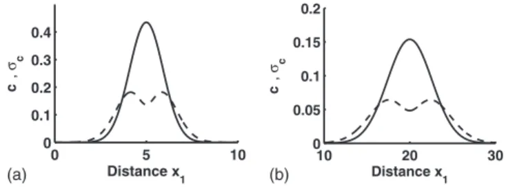
Figure 2shows the mean concentration c¯共x₁, t兲 and stan-dard deviation ␴c共x1, t兲 at t=500␶D and t = 2⫻103␶D. Note

the double peak in the standard deviation, which indicates that the region of maximum uncertainty and maximum aver-age concentration do not coincide. The general shapes of the curves change proportionally in time 共reflecting the fact that the ratio between D11共t兲 and D12共t兲 is constant兲.

D. Numerical simulations

The explicit analytical expression共31兲 for the

concentra-tion variance is compared to Monte Carlo simulaconcentra-tions. We use particle tracking simulations in two-dimensional random shear flow. The simulated flow field is organized in layers of constant thickness l. The velocity within each layer is con-stant, drawn from a Gaussian distribution with unit mean and variance. For transverse scales much larger than the thick-ness of a layer, the correlation is approximately delta 共e.g., 关33兴兲. Solute transport is simulated by random walk particle

tracking. Initial positions are uniformly distributed along a vertical line source, whose length is 104_{l. Within each} stra-tum 103 _{particles are released, which gives a total of 10}7 simulated particle trajectories. Averages are then taken over the projected partial distributions that evolve from the strata. The implementation of the particle tracking method is de-scribed in detail in 关35兴. Equivalently, we considered

aver-ages over particle distributions consisting of 103 _particles evolving from point sources in 104 different realizations of

0 5 10 0 0.1 0.2 0.3 0.4 Distance x 1 c , σc 10 20 30 0 0.05 0.1 0.15 0.2 Distance x₁ c , σc (b) (a)

FIG. 2. Evolution of the mean concentration 共solid兲 and vari-ance共dashed兲 at two times 共a兲 t=500␶Dand共b兲 t=2⫻103␶Dfor a

variance of␴_u2= 1.

DENTZ et al. PHYSICAL REVIEW E 80, 036306共2009兲

the flow field. The results are identical as a consequence of the ergodicity of the random velocity field. In the following, we present only the results obtained for a long line source in a single realization.

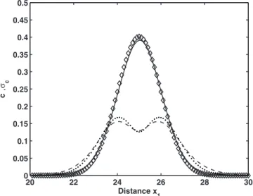
A comparison of the results from the numerical simula-tions and the corresponding analytical solusimula-tions are shown in Fig.3. As one can see, the analytical and numerical solutions are in good agreement, which is not surprising as the derived expressions for the multipoint concentration moments are ex-act for an infinite medium. Several other simulations varying the modeling parameters were run, yielding similar results. Note that the mean concentration obtained by numerical simulations agrees almost perfectly with the predicted behav-ior, while for the variance there are slight deviations. This can be traced back to the fact that the latter is much more sensitive to noise.

IV. SUMMARY AND CONCLUSIONS

We present a Lagrangian methodology for deriving the multipoint concentration statistics in Gaussian distributed random shear flow and determine explicit expressions for the multipoint concentration moments. The specific model under consideration has been frequently considered in the literature to study non-Fickian diffusion and the resulting effective particle densities共e.g., 关3,21,22,24,25,28兴兲. In fact, the

effec-tive dispersion coefficient evolves anomalously with the square root of time. In a stochastic modeling approach, the mean concentration distribution of a solute is defined by en-semble averaging of the concentration distribution originat-ing from an instantaneous point injection in one realization of the random flow field.

Alternatively, for an ergodic random flow field, the mean behavior can be obtained by considering transport in a single

realization for a solute that originates from a line source perpendicular to the stratification that is much larger than the characteristic scale of flow stratification. In this case the mean behavior is obtained by projecting the partial plumes evolving from points along the vertical line source and aver-aging of the source distribution 关28兴. The vertical particle

movements describe a Brownian motion and are independent of the longitudinal movement. Thus the effective distribution is given by the product of the vertically projected effective density and a Gaussian density representing the vertical dis-tribution. Therefore, it is sufficient to focus on the vertical projection of the effective particle distribution. Dentz et al. 关28兴 showed that the effective, or mean, particle movements

can be represented by a correlated random walk, where the noise correlation is uniquely defined by the Lagrangian ve-locity correlation function. The mean particle distribution is then given by the density of this random walk. Being a cor-related random walk, the process is non-Markovian. Here we extend this methodology to determine the full concentration statistics as given by the explicit analytical expressions for the multipoint moments of the concentration distribution. This yields a full statistical characterization of the non-Markovian effective particle dynamics. We obtain multi-Gaussian distribution densities for the n-point densities. These are completely characterized by 共i兲 the mean particle velocity,共ii兲 the single particle velocity correlation, and 共iii兲 the two-particle velocity correlation.

We then study the concentration variance as a simple measure for the uncertainty of concentration values and for the self-averaging properties of the particle distribution. The concentration variance is characterized by a double peak and decreases with time and distance from the center of mass. The relative concentration, in contrast, increases both with distance from the mean center of mass and time. This implies that the low concentration values are particularly uncertain, or in other words, that the low probabilities of finding a particle at a given position at a given time, are very uncer-tain. The relative variance is constant at the center of mass of the mean distribution which indicates that the probability of the bulk of the particles, or the highest concentration, is sub-ject to a basically constant uncertainty.

These results have some practical relevance because ex-perimentally determined concentration values and particle densities are often obtained as space and/or time averages and the observed mean behavior is often found to be super-diffusive. The presented work considers a model that gives some insight in the mechanism that can lead to such behavior and provides a methodology to quantify uncertainty and in fact the full concentration statistics.

In conclusion, by focusing on a relatively simple random flow model, this work sheds some new light and provides novel insights on the features and possible limitations of sto-chastic transport models in random flows. The presented methodology and the results obtained may have some impact for risk assessment studies and extreme value analysis.

20 22 24 26 28 30 0 0.05 0.1 0.15 0.2 0.25 0.3 0.35 0.4 0.45 0.5 Distance x 1 c , σ c

FIG. 3. A comparison between the numerical concentration共-兲 and standard deviation共- -兲 against the analytical values of concen-tration 共〫兲 and standard deviation 共·兲 for ␴_u2= 1 and t = 2.5 ⫻105_␶

关1兴 J. P. Bouchaud and A. Georges, Phys. Rep. 195, 127 共1990兲. 关2兴 B. Berkowitz, A. Cortis, M. Dentz, and H. Scher, Rev.

Geo-phys. 44, RG2003共2006兲.

关3兴 W. R. Young and S. Jones, Phys. Fluids A 3, 1087 共1991兲. 关4兴 E. Frey and K. Kroy, Ann. Phys. 14, 20 共2005兲.

关5兴 J. Carrera, J. Contam. Hydrol. 13, 23 共1993兲.

关6兴 B. Berkowitz and H. Scher, Transp. Porous Media 42, 241 共2001兲.

关7兴 D. Tartakovsky, Geophys. Res. Lett. 34, L05404 共2007兲. 关8兴 D. Bolster, M. Barahona, M. Dentz, D. Fernandez-Garcia, X.

Sanchez-Vila, P. Trinchero, C. Valhondo, and D. M. Tartak-ovsky, Water Resour. Res. 45, W06413共2009兲.

关9兴 J. A. Neufeld and H. E. Huppert, J. Fluid Mech. 625, 353 共2009兲.

关10兴 D. Bolster, M. Dentz, and J. Carrera, Water Resour. Res. 45, W05408共2009兲.

关11兴 S. Pope, Turbulent Flows 共Cambridge University Press, Cam-bridge, England, 2000兲.

关12兴 R. Kubo, M. Toda, and N. Hashitsume, Statistical Physics II, Non-Equilibrium Statistical Mechanics共Springer-Verlag, Ber-lin, Heidelberg, 1991兲.

关13兴 V. Kapoor and L. W. Gelhar, Water Resour. Res. 30, 1775 共1994兲.

关14兴 V. Kapoor and P. K. Kitanidis, Water Resour. Res. 34, 1181 共1998兲.

关15兴 V. Kapoor and P. K. Kitanidis, Stoch. Hydrol. Hydraul. 11, 397共1997兲.

关16兴 W. Graham and D. McLaughlin, Water Resour. Res. 25, 215 共1989兲.

关17兴 S. Fedotov, M. Ihme, and H. Pitsch, Phys. Rev. E 71, 016310 共2005兲.

关18兴 Z. Warhaft, Annu. Rev. Fluid Mech. 32, 203 共2000兲. 关19兴 E. Caroni and V. Fiorotto, Transp. Porous Media 59, 19

共2005兲.

关20兴 O. A. Cirpka, R. L. Schwede, J. Luo, and M. Dentz, J. Contam. Hydrol. 98, 61共2008兲.

关21兴 G. Matheron and G. de Marsily, Water Resour. Res. 16, 901 共1980兲.

关22兴 J. P. Bouchaud, A. Georges, J. Koplik, A. Provata, and S. Redner, Phys. Rev. Lett. 64, 2503共1990兲.

关23兴 S. Redner, Physica A 168, 551 共1990兲.

关24兴 G. Zumofen, J. Klafter, and A. Blumen, Phys. Rev. A 42, 4601 共1990兲.

关25兴 S. N. Majumdar, Phys. Rev. E 68, 050101共R兲 共2003兲. 关26兴 O. Güven, F. Molz, and J. G. Melville, Water Resour. Res. 20,

1337共1984兲.

关27兴 A. Fiori and G. Dagan, Transp. Porous Media 47, 81 共2002兲. 关28兴 M. Dentz, T. LeBorgne, and J. Carrera, Phys. Rev. E 77,

020101共R兲 共2008兲.

关29兴 H. Risken, The Fokker-Planck Equation 共Springer, Heidelberg, New York, 1996兲.

关30兴 A. Fiori and G. Dagan, J. Contam. Hydrol. 45, 139 共2000兲. 关31兴 E. Morales-Casique, S. P. Neuman, and A. Guadagnini, Adv.

Water Resour. 29, 1238共2005兲.

关32兴 M. Clincy and H. Kinzelbach, J. Phys. A 34, 7141 共2001兲. 关33兴 V. Zavala-Sánchez, M. Dentz, and X. Sanchez-Vila, Adv.

Wa-ter Resour. 32, 635共2008兲.

关34兴 M. Dentz, H. Kinzelbach, S. Attinger, and W. Kinzelbach, Wa-ter Resour. Res. 36, 3591共2000兲.

关35兴 T. Le Borgne, J. R. De Dreuzy, P. Davy, and O. Bour, Water Resour. Res. 43, W02419共2007兲.

DENTZ et al. PHYSICAL REVIEW E 80, 036306共2009兲