A monitoring system for spatiotemporal electrical self-potential measurements in cryospheric environments

(1)

Supplement of Geosci. Instrum. Method. Data Syst., 9, 317–336, 2020 https://doi.org/10.5194/gi-9-317-2020-supplement

Supplement of

A monitoring system for spatiotemporal electrical self-potential

measure-ments in cryospheric environmeasure-ments

Maximilian Weigand et al.

Correspondence to:Maximilian Weigand (mweigand@geo.uni-bonn.de)

(2)

S1: Measurement ﬂowchart

schedule measured parameter action

daily contact resistances measure

hourly for Vbat > 12.3 V

or

6-hourly for Vbat< 12.2 V

electrode temperatures measure

5 am - 8 pm 10 min, if Vbat> 12.6 V hourly, if Vbat > 12.3 V; < 12.5V 6-hourly, if Vbat< 12.2 V SP-voltages battery voltage air-temperature solar voltage 8 am - 5 pm 30 min, if Vbat> 12.6 V hourly, if Vbat > 12.3 V; < 12.5V 6-hourly, if Vbat< 12.2 V SP-voltages battery voltage air-temperature solar voltage

6-hourly send data by email

daily update logger time to UTC using ntp

Table 1: Measurement schedule of the measurement system. Note that data upload and ntp schedules have been varied over time to reduce power consumption and increase system reliability

(3)

S2: Internal signal ﬂow

Figure 1: Signal ﬂow in the measurement system. The incoming signal lines (upper left, red) are routed and multiplexed from the incoming cables using custom-made PCB boards, ﬁnally connecting to multiple data logger input channels (bottom, green).

(4)

Figure 2: Lightning protection and low-pass circuit, applied to each SP electrode input line (as such this circuit was duplicated 20 times, using 4 pcb boards with 5 circuits each). The electrode and temperature signals arrive into the SP system via ethernet cables (one electrode group per cable), which are then connected to an ethernet panel (see Fig. 5 of manuscript, lower right corner). From here on each electrode group is routed using a short ethernet cable to to the lightning protection circuit.

(5)

TEMP5_L4 TEMP5_L3 TEMP5_L2 TEMP5_L1 TEMP4_L4 TEMP4_L3 TEMP4_L2 TEMP4_L1 TEMP3_L4 TEMP3_L3 TEMP3_L2 TEMP3_L1 TEMP2_L4 TEMP2_L3 TEMP2_L2 TEMP2_L1 TEMP1_L4 TEMP1_L3 TEMP1_L2 TEMP1_L1

POTENTIAL1 POTENTIAL2 POTENTIAL3 POTENTIAL4 POTENTIAL5

1 2 3 4 5 6 7 8 SENSOR1 0446200002 DT80_CH1A DT80_CH1B DT80_CH1C DT80_CH1D 1 2 3 4 5 6 7 8 TO_MULTIPLEXER1 0446200002 1 2 3 4 5 6 7 8 SENSOR2 0446200002 1 2 3 4 5 6 7 8 SENSOR3 0446200002 1 2 3 4 5 6 7 8 SENSOR4 0446200002 1 2 3 4 5 6 7 8 SENSOR5 0446200002 DT80_CH2A DT80_CH2B DT80_CH2C

DT80_CH2D DT80_CH3D DT80_CH3C DT80_CH3B DT80_CH3A DT80_CH4D DT80_CH4C DT80_CH4B DT80_CH4A DT80_CH5D DT80_CH5C DT80_CH5B DT80_CH5A

brown blue white/orange green

white/green

one input of rsplit circuit

cable input from outside

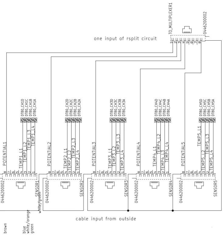
Figure 3: Input splitter diagram, splitting temperature and SP signal lines. Electrode group signals arrive from the lightning protection circuit at the bottom and are then routed either directly to the corresponding logger inputs for temperature measurements (groups of four output in the cen-ter), or, in groups of 5 SP signals, are routed to the resistance split circuit (ethernet output at the top). This circuit was duplicated four time to accommodate the 20 electrode groups.

(6)

ELECTRODE1 ELECTRODE1 ELECTRODE2 ELECTRODE2 ELECTRODE3 ELECTRODE3 ELECTRODE4 ELECTRODE4 ELECTRODE8 ELECTRODE8 ELECTRODE5 ELECTRODE5 ELECTRODE10 ELECTRODE10 ELECTRODE15 ELECTRODE15 ELECTRODE20 ELECTRODE20 ELECTRODE16 ELECTRODE16 ELECTRODE17 ELECTRODE17 ELECTRODE18 ELECTRODE18 ELECTRODE19 ELECTRODE19 ELECTRODE11 ELECTRODE11 ELECTRODE12 ELECTRODE12 ELECTRODE13 ELECTRODE13 ELECTRODE14 ELECTRODE14 ELECTRODE6 ELECTRODE6 ELECTRODE7 ELECTRODE7 ELECTRODE9 ELECTRODE9 1 2 3 4 5 6 7 8 IN3 0446200002 1 2 3 4 5 6 7 8 IN4 0446200002 1 2 3 4 5 6 7 8 IN2 0446200002 1 2 3 4 5 6 7 8 IN1 0446200002 1 2 3 4 5 6 7 8 OUT1 _0446200002 1 2 3 4 5 6 7 8 OUT2 _0446200002 1 2 3 4 5 6 7 8 OUT3 _0446200002 1 2 3 4 5 6 7 8 OUT4 _0446200002 3011A 3011B 3011C 3011D 3021A 3021B 3021C 3021D 3031A 3031B 3031C 3031D 3041A 3041B 3041C 3041D 3051A 3051B 3051C 3051D 3061A 3061B 3061C 3061D 3071A 3071B 3071C 3071D 3081A 3081B 3081C 3081D 3091A 3091B 3091C 3091D 3101A 3101B 3101C 3101D 3111A 3111B 3111C 3111D 3121A 3121B 3121C 3121D 3131A 3131B 3131C 3131D 3141A 3141B 3141C 3141D 3151A 3151B 3151C 3151D 3161A 3161B 3161C 3161D 3171A 3171B 3171C 3171D 3181A 3181B 3181C 3181D 3191A 3191B 3191C 3191D 3201A 3201B 3201C 3201D EXTRA1A EXTRA1B EXTRA1C EXTRA1D

inputs from input_split circuit

to multiplexer circuit

Figure 4: Resistance multiplexer diagram, multiplexing electrode lines to separate inputs for resistance measure-ments. SP signals arrive at the top from the four resistance splitting circuits. Signals are then multiplexed to certain logger inputs for resistance measurements (outputs in the center of the circuit, note that two outputs are always short circuited). The SP signals are directly routed to the outputs at the bottom for

(7)

ELECTRODE20 ELECTRODE20 ELECTRODE20 ELECTRODE19 ELECTRODE19 ELECTRODE18 ELECTRODE18 ELECTRODE17 ELECTRODE17 ELECTRODE17 ELECTRODE17 ELECTRODE1

ELECTRODE1 ELECTRODE1 ELECTRODE1 ELECTRODE1 ELECTRODE1 ELECTRODE1

ELECTRODE16

ELECTRODE16 ELECTRODE16 ELECTRODE16 ELECTRODE16

ELECTRODE2 ELECTRODE2 ELECTRODE2 ELECTRODE3 ELECTRODE3 ELECTRODE3 ELECTRODE4 ELECTRODE4 ELECTRODE4 ELECTRODE5 ELECTRODE5 ELECTRODE5 ELECTRODE6 ELECTRODE6 ELECTRODE6 ELECTRODE7 ELECTRODE7 ELECTRODE7 ELECTRODE8 ELECTRODE8 ELECTRODE8 ELECTRODE9 ELECTRODE9 ELECTRODE9 ELECTRODE10 ELECTRODE10 ELECTRODE10 ELECTRODE11 ELECTRODE11 _ELECTRODE11 ELECTRODE12 ELECTRODE12 ELECTRODE12 ELECTRODE13 ELECTRODE13 ELECTRODE13 ELECTRODE14 ELECTRODE14 ELECTRODE14 ELECTRODE15 ELECTRODE15 ELECTRODE15 1 2 3 4 5 6 7 8 IN_E1_E5 1 2 3 4 5 6 7 8 IN_E6_E10 E1_1A E1_1B E1_1C

E1_1D E1_2D E1_2C E1_2B E1_2A E1_3D E1_3C E1_3B E1_3A E1_4D E1_4C E1_4B E1_4A E1_5D E1_5C E1_5B E1_5A E16_1D E16_1C E16_1B E16_1A E16_2D E16_2C E16_2B E16_2A E16_3D E16_3C E16_3B E16_3A E16_4D E16_4C E16_4B E16_4A E16_5D E16_5C E16_5B E16_5A

1 2 3 4 5 6 7 8 IN_E11-E15 1 2 3 4 5 6 7 8 IN_E16-E20 E1_6A E1_6B E1_6C

E1_6D E16_6D E16_6C E16_6B E16_6A E20_1D E20_1C E20_1B E20_1A E19_1D E19_1C E19_1B E19_1A

* Multiplexer Inputs Electrode Inputs ELECTRODE 18 ELECTRODE 19 ELECTRODE 19 ELECTRODE17

Figure 5: Multiplexer circuit diagram multiplexing SP input lines to speciﬁc inputs of the data logger. Each electrode is connected to one port on the bottom (“Electrode inputs”) and then routed to one or more of the data logger multiplexer channels on the top (“Multiplexer Inputs”). Note that each logger input channel consists of four physical inputs, allowing for a variety of measurement combinations.

(8)

S3: Electrode matching

15.50 15.75 16.00 16.25 16.50 16.75 17.00 17.25 time [hours] 6 4 2 0 2 Voltage [mV]

before selection

21.20 21.25 21.30 21.35 21.40 21.45 time [hours]

after selection

Figure 6: Test measurements of base-line electrical offsets in saline solution. Left: Voltage measure-ments for 20 randomly selected SP electrodes, right: Voltage measuremeasure-ments for 20 matched SP electrodes

The absolute potentials of SP electrodes changes with age, chemical environment, and usage history. As such, it is commonly advised to check the baseline potential difference between electrodes before measurements commence (e.g., Corwin, 1989), in order to not confuse the offsets with process-based signals. Out of the pool of available SP electrodes, we initially selected 20 random electrodes. This yielded voltages with respect to electrodes 1 and 16 of down to -5.4 mV (Fig. 6, left). Following this, electrodes were selected out of the available pool to minimize this offset voltage, resulting in a maximum voltage difference of±1 mV (Fig. 6, right).

(9)

S4: SP data ﬁltering

Figure 7: Data processing steps applied to SP data presented in this study, shown for the dipole E5-E1. Captured SP data presented in this study exhibits quite large noise levels (e.g., Fig. 7a). This is caused by aliasing artifacts, as well as anthropogenic noise due to the operation of the cable-car to the summit and corresponding touristic operations. As such data was processed as follows: First, data was resampled to 30 minute intervals, using linear interpolation and averaging. The effect of this operation is exemplarily shown in Fig. 7b. Depending on the speciﬁc application, in the following various rolling mean ﬁlters are

(10)

applied to the data, serving as simple, yet crude, low-pass ﬁlters. The effects of various window sizes is presented in Fig. 7c.

We fully acknowledge that the use of rolling average filters is not necessarily optimal for frequency-domain filtering. In addition, other filters, such as the rolling median or the alpha-trimmed-mean filter (Gersztenkorn and Scales, 1988), are known to better preserve transient spikes. Yet, in the present study we only aimed at presenting certain characteristics or concepts, which allowed us to use the robust and simple rolling average filter.

(11)

S5: Wavelet analysis of noise data

Figure 8: Wavelet analysis of the noise measurements 2019

In order to gain more information on spatio-temporal spectral content, a wavelet-based analysis (e.g., Grinsted et al., 2004) was conducted on the noise measurements conducted in 2019. The analysis shows strong 30 minute components during the day, a section of a few hours with 60 minute components just before night, and no signiﬁcant spectral components during night-time hours (Fig. 8).

The analysis was conducted using the waipy software package (originally from https://github.com/ mabelcalim/waipy, fork used here: https://github.com/m-weigand/waipy).

(12)

1 Data Logger programming

' DT80M program Schilthorn SP system 2017

'reset the logger

session stop session clear cevtlog cerrlog

deldjob=*archive=y

deljob *

' restore settings to default factorydefaults

'some debug infos

profile parametersP56=1

' we operate on UTC profile locale time_zone=+0H

'sim:

profile modemservice=gsm_preferred

profile modemMIN_SIGNAL_FOR_DATA_DBM=-110

' coop mobile CH internet settings profile modem pin=XXXX

profile modem apn=click profile modem apn_account="" profile modem apn_password="" profile modem_session smtp_server=XXXX profile modem_session smtp_account=XXXX profile modem_session smtp_password=XXXX

PROFILE UNLOAD FTP_RETRIES=10

'mains frequency[Hz]

profile parametersp11=20

' sleep while on power, but not if USB is connected profile parameters p15=1

'5V power outputwhilethe measurement system is on

PWR5V=1

' should prevent some debug messages profile http_server enable_wdg=no

'reduce power by disabling ethernet

profile ethernetenable=no

profile ethernetip_address=192.168.21.10

profile ethernetsubnet_mask=255.255.255.0

' define functions for the yellow button profile function f1_label = "mail data" profile function f1_command = "copyd start=new \

dest=mailto:XX@XX.XX?&subject=sch17_01&priority=high&interface=modem \ format=dbd merge=N"

profile function f2_label = "PWR5V" profile function f2_command = "PWR5V=1"

(13)

profile function f3_label = "session signal" profile function f3_command = "session signal"

profile function f4_label = "download all"

profile function f4_command = "COPYD job=* dest=a: merge=N format=dbd; \ servicedata a:\\\\servicedata.txt; removemedia"

profile function f5_label = "servicedata to usb"

profile function f5_command = "SERVICEDATA a:\\\\servicedata.txt"

profile modem_session sTART_CRON=0:5:10:*:*:* profile modem_session stop_CRON=0:20:10:*:*:* profile modem_session timing_control=cron

'[seconds : minutes : hours : day : month : weekday]

BEGIN"sch17_01" ' measure voltages RA"SPV"("B:",data:ov:370D)10M 101*V("E02-E01",ES10) 101+V("E03-E01",ES10) 101-V("E04-E01",ES10) 102*V("E05-E01",ES10) 102+V("E06-E01",ES10) 102-V("E07-E01",ES10) 103*V("E08-E01",ES10) 103+V("E09-E01",ES10) 103-V("E10-E01",ES10) 104*V("E11-E01",ES10) 104+V("E12-E01",ES10) 104-V("E13-E01",ES10) 105*V("E14-E01",ES10) 105+V("E15-E01",ES10) 105-V("E16-E01",ES10) 106*V("E19-E01",ES10) 106+V("E20-E01",ES10) 107*V("E02-E16",ES10) 107+V("E03-E16",ES10) 107-V("E04-E16",ES10) 108*V("E05-E16",ES10) 108+V("E06-E16",ES10) 108-V("E07-E16",ES10) 109*V("E08-E16",ES10) 109+V("E09-E16",ES10) 109-V("E10-E16",ES10) 110*V("E11-E16",ES10) 110+V("E12-E16",ES10) 110-V("E13-E16",ES10) 111*V("E14-E16",ES10) 111+V("E15-E16",ES10) 111-V("E17-E16",ES10) 112*V("E18-E16",ES10) 113*V("E18-E20",ES10) 113+V("E19-E20",ES10) 114*V("E17-E19",ES10) 115*HV("Battery") 116PT385("TempOutside",4W) 117*HV("RH_INSIDE") 118*HV("RH_OUTSIDE") 119*HV("RAIN") 120*HV("SOLAR") 13

(14)

VEXT 'measure temperatures RB"TEMPS"("B:",data:ov:370D)1H 201*V("T1Voltage")201PT385("Temp01",4W) 202*V("T2Voltage")202PT385("Temp02",4W) 203*V("T3Voltage")203PT385("Temp03",4W) 204*V("T4Voltage")204PT385("Temp04",4W) 205*V("T5Voltage")205PT385("Temp05",4W) 206*V("T6Voltage")206PT385("Temp06",4W) 207*V("T7Voltage")207PT385("Temp07",4W) 208*V("T8Voltage")208PT385("Temp08",4W) 209*V("T9Voltage")209PT385("Temp09",4W) 210*V("T10Voltage")210PT385("Temp10",4W) 211*V("T11Voltage")211PT385("Temp11",4W) 212*V("T12Voltage")212PT385("Temp12",4W) 213*V("T13Voltage")213PT385("Temp13",4W) 214*V("T14Voltage")214PT385("Temp14",4W) 215*V("T15Voltage")215PT385("Temp15",4W) 216*V("T16Voltage")216PT385("Temp16",4W) 217*V("T17Voltage")217PT385("Temp17",4W) 218*V("T18Voltage")218PT385("Temp18",4W) 219*V("T19Voltage")219PT385("Temp19",4W) 220*V("T20Voltage")220PT385("Temp20",4W)

REFT 1REFT 2REFT 3REFT

' Resistances RC"RES"("B:",data:ov:1MB)[0:5:6] 301R("R01-02",III) 301*V("V01-02") 302R("R02-03",III) 302*V("V02-03") 303R("R03-04",III) 303*V("V03-04") 304R("R04-08",III) 304*V("V04-08") 305R("R01-05",III) 305*V("V01-05") 306R("R05-06",III) 306*V("V05-06") 307R("R06-07",III) 307*V("V06-07") 308R("R07-08",III) 308*V("V07-08") 309R("R08-12",III) 309*V("V08-12") 310R("R05-09",III) 310*V("V05-09") 311R("R09-10",III) 311*V("V09-10") 312R("R10-11",III) 312*V("V10-11") 313R("R11-12",III) 313*V("V11-12") 314R("R12-16",III) 314*V("V12-16") 315R("R09-13",III) 315*V("V09-13") 316R("R13-14",III) 316*V("V13-14") 317R("R14-15",III) 317*V("V14-15") 318R("R15-16",III) 318*V("V15-16") 319R("R01-19",III) 319*V("V01-19") 320R("R16-17",III) 320*V("V16-17") VLITH R100 VREF VZERO

'at night we increase measurement intervals

RD[0:5:20]IF(115*HV>12.6){RA30M}

RE[0:5:4]IF(115*HV>12.6){RA10M}

RF6H

DO{copydstart=new2dest=mailto:XXX@XXX.XX?&\

subject=sch17_01&priority=high&interface=modemformat=dbdmerge=N}

(15)

' Alarm section RH2H

ALARM1(115*HV>12.6)"Battery larger than 12.6 V"{RA10M RB1H}

ALARM2(115*HV><12.3,12.5)"Battery below 12.5, but above 12.3 V"{RA1H RB1H} ALARM3(115*HV<12.2)"Battery below 12.2 V"{RA6H RB6H}

DO{PWR5V=1} 'update clock RX[0:10:11:*:*:*]do{ntp} LOGON END ' disable debug profile parametersP56=0

Listing 1: Programming of the DataTaker DT80M – Series 4 logger

(16)

S6: Laboratory Experiment

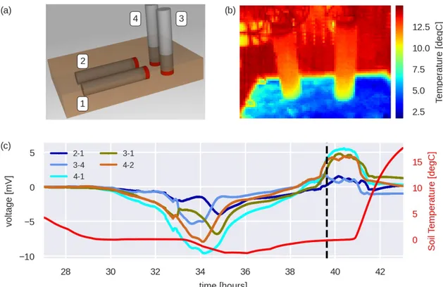
Figure 9: Laboratory experiment investigating electrode effects during freezing and thawing. a) Sketch of experimental setup. The container is 30 cm in length, 20 cm in depth, and 5 cm high. Electrodes are shown in gray, with the wood membranes in contact with the surrounding highlighted in red and assigned electrode numbers in white boxes. b) Thermal image (surface temperatures) during thawing c) Electrical voltages and soil temperatures; vertical black line indicates time of thermal image in b).

(17)

References

Corwin, R.: Data quality for engineering self-potential surveys, in: Detection of Subsurface Flow Phenomena, edited by Merkler, G.-P., Militzer, H., Hötzl, H., Armbruster, H., and Brauns, J., pp. 49–72, Springer Berlin Heidelberg, Berlin, Heidelberg, https://doi.org/10.1007/BFb0011630, 1989.

Gersztenkorn, A. and Scales, J. A.: Smoothing seismic tomograms with alpha-trimmed means, Geophysical Journal International, 92, 67–72, https://doi.org/10.1111/j.1365-246X.1988.tb01121.x, 1988.

Grinsted, A., Moore, J., and Jevrejeva, S.: Application of the cross wavelet transform and wavelet coherence to geo-physical time series, Nonlinear processes in geophysics, 11, 561–566, https://doi.org/10.5194/npg-11-561-2004, 2004.