Constraints from observations and modeling on atmosphere–
surface exchange of mercury in eastern North America
The MIT Faculty has made this article openly available. Please share
how this access benefits you. Your story matters.
Citation
Song, Shaojie, Noelle E. Selin, Lynne E. Gratz, Jesse L. Ambrose,
Daniel A. Jaffe, Viral Shah, Lyatt Jaeglé, et al. “Constraints from
Observations and Modeling on Atmosphere–surface Exchange
of Mercury in Eastern North America.” Elementa: Science of the
Anthropocene 4 (April 8, 2016): 000100. © 2016 Song et al
As Published
http://dx.doi.org/10.12952/journal.elementa.000100
Publisher
University of California Press
Version
Final published version
Citable link
http://hdl.handle.net/1721.1/109353
Terms of Use
Creative Commons Attribution
Constraints from observations and modeling
on atmosphere–surface exchange of mercury
in eastern North America
Atmosphere-surface exchange of mercury in eastern North AmericaShaojie Song1*• Noelle E. Selin1,2• Lynne E. Gratz3• Jesse L. Ambrose4• Daniel A. Jaffe5,6• Viral Shah6•
Lyatt Jaeglé6• Amanda Giang2• Bin Yuan7,8• Lisa Kaser9• Eric C. Apel9• Rebecca S. Hornbrook9•
Nicola J. Blake10• Andrew J. Weinheimer9• Roy L. Mauldin III11,12• Christopher A. Cantrell11• Mark
S. Castro13• Gary Conley14• Thomas M. Holsen15• Winston T. Luke16• Robert Talbot17
1Department of Earth, Atmospheric and Planetary Sciences, Massachusetts Institute of Technology, Cambridge,
Massachusetts, United States
2Institute for Data, Systems and Society, Massachusetts Institute of Technology, Cambridge, Massachusetts, United
States
3Environmental Program, Colorado College, Colorado Springs, Colorado, United States
4College of Engineering and Physical Sciences, University of New Hampshire, Durham, New Hampshire, United
States
5School of Science, Technology, Engineering and Mathematics, University of Washington, Bothell, Washington,
United States
6Department of Atmospheric Sciences, University of Washington, Seattle, Washington, United States
7Chemical Sciences Division, Earth System Research Laboratory, National Oceanic and Atmospheric Administration,
Boulder, Colorado, United States
8Cooperative Institute for Research in Environmental Sciences, University of Colorado, Boulder, Colorado, United
States
9Atmospheric Chemistry Observations & Modeling Laboratory, National Center for Atmospheric Research,
Boulder, Colorado, United States
10Department of Chemistry, University of California, Irvine, Irvine, California, United States
11Department of Atmospheric and Oceanic Sciences, University of Colorado, Boulder, Colorado, United States 12Department of Physics, University of Helsinki, Helsinki, Finland
13Center for Environmental Science, Appalachian Laboratory, University of Maryland, Frostburg, Maryland,
United States
14Center for Air Quality, Ohio University, Athens, Ohio, United States
15Department of Civil and Environmental Engineering, Clarkson University, Potsdam, New York, United States 16Air Resources Laboratory, National Oceanic and Atmospheric Administration, College Park, Maryland, United States 17Department of Earth and Atmospheric Sciences, University of Houston, Houston, Texas, United States
*song33@mit.edu
Abstract
Atmosphere–surface exchange of mercury, although a critical component of its global cycle, is currently poorly constrained. Here we use the GEOS-Chem chemical transport model to interpret atmospheric Hg0
(gaseous elemental mercury) data collected during the 2013 summer Nitrogen, Oxidants, Mercury and Aerosol Distributions, Sources and Sinks (NOMADSS) aircraft campaign as well as ground- and ship-based observations in terms of their constraints on the atmosphere–surface exchange of Hg0 over eastern North
America. Model–observation comparison suggests that the Northwest Atlantic may be a net source of Hg0,
with high evasion fluxes in summer (our best sensitivity simulation shows an average oceanic Hg0 flux of
3.3 ng m-2 h-1 over the Northwest Atlantic), while the terrestrial ecosystem in the summer of the eastern
United States is likely a net sink of Hg0 (our best sensitivity simulation shows an average terrestrial Hg0 flux
of -0.6 ng m-2 h-1 over the eastern United States). The inferred high Hg0 fluxes from the Northwest Atlantic
may result from high wet deposition fluxes of oxidized Hg, which are in turn related to high precipitation
Domain Editor-in-Chief
Joel D. Blum, University of Michigan
Guest Editor
Ian Michael Hedgecock, CNR Institute for Atmospheric Pollution Research
Knowledge Domains
Atmospheric Science Earth & Environmental Science
Article Type
Research Article
Part of an Elementa Special Feature
Monitoring, measuring and modeling atmospheric mercury and air-surface exchange – are we making progress?
Received: November 23, 2015 Accepted: March 10, 2016 Published: April 8, 2016
rates in this region. We also find that increasing simulated terrestrial fluxes of Hg0 in spring compared to
other seasons can better reproduce observed seasonal variability of Hg0 concentration at ground-based sites
in eastern North America.
Introduction
Mercury (Hg) is a trace metal that has adverse effects on human health and the environment (Driscoll et al., 2013). Unlike most other metals, mercury in the lower atmosphere exists primarily in its elemental form (Hg0;
also known as gaseous elemental mercury, GEM), which is volatile and poorly soluble (Lin and Pehkonen, 1999). The major loss pathway of atmospheric Hg0 is via oxidation to its oxidized state (HgII), a much more
soluble form that partitions between the gas and particle phases, and subsequently undergoes dry and wet deposition (Lindberg et al., 2007; Selin, 2009). After being deposited on land and water surfaces, HgII can be
reduced photochemically and/or biochemically to Hg0, which can be reemitted back to the atmosphere (Selin
et al., 2008). The atmosphere–surface exchange of Hg0 is thus bidirectional: both evasion (upward) and dry
deposition (downward) occur at the interface (Gustin and Lindberg, 2005; Xu et al., 1999). Wet deposition of Hg0 is insignificant due to its low solubility (Maestas, 2011). A positive (negative) net flux indicates
that Hg0 evasion exceeds (is lower than) its dry deposition (Gustin et al., 2006). Hg0 exchange fluxes are
important components of global Hg emissions, which also include anthropogenic sources, geogenic activities, and biomass burning (Pirrone et al., 2010). Despite their global importance, Hg0 fluxes from terrestrial and
oceanic surfaces remain poorly constrained at global and regional scales, leading to considerable uncertainty in our understanding of the biogeochemical Hg cycle.
Based on field flux measurements and modeling studies, it remains unclear whether the global terrestrial ecosystem acts as a net source or a net sink of atmospheric Hg0. More than 100 field studies have been
conducted since the 1970s to measure terrestrial Hg0 fluxes from various surface types (e.g., bare soil, forest,
grassland, and snow/ice) and to determine environmental factors influencing Hg0 exchange (e.g., Lindberg
and Turner, 1977; Xiao et al., 1991; Poissant et al., 2004; Ferrari et al., 2005; Obrist et al., 2005; Fritsche et al., 2008; Fu et al., 2010). A recent global database summarizing these studies shows a high variability in measured Hg0 fluxes over terrestrial surfaces (Agnan et al., 2016). Small-scale (<0.1 to 103 m2) measurements,
although unevenly distributed in time and among regions and landscapes, have been extrapolated to estimate terrestrial Hg0 fluxes at a global scale (for example, (1000–3410 Mg yr-1, Mason, 2009); -2810 to 4650 Mg yr-1
(50% uncertainty range; Agnan et al., 2016)). Agnan et al. (2016) has suggested that the largest uncertainty in estimating global terrestrial Hg0 fluxes arises from the forest ecosystem, which has a median flux of -59
Mg yr-1 (a small net sink) with a very large 50% uncertainty range (-2580–3276 Mg yr-1).
Most atmospheric mercury models treat Hg0 emission from, and dry deposition to, land separately. Dry
deposition is typically simulated using a resistance-in-series scheme (Wesely, 1989; Zhang et al., 2009). Some models calculate soil emissions with empirical equations involving important controlling factors such as solar radiation, temperature, and substrate Hg concentrations (Selin et al., 2008; Holmes et al., 2010; Lei et al., 2013; Lin et al., 2010; Shetty et al., 2008). Terrestrial emissions in some other models are mapped according to biogenic CO emission and/or historical Hg deposition and scaled by global Hg budgets (Dastoor et al., 2015; Chen et al., 2015; Jung et al., 2009). Simulated global Hg0 fluxes from terrestrial surfaces range from
-1300 to 3500 Mg yr-1 (Holmes et al., 2010; Chen et al., 2015; Lei et al., 2013; Corbitt et al., 2011;
Smith-Downey et al., 2010; Kikuchi et al., 2013; Amos et al., 2013, 2014; De Simone et al., 2014). Net Hg0 fluxes
from the contiguous United States may also be positive or negative based on flux scaling methods (-183 to 269 Mg yr-1, 50% uncertainty range; Agnan et al., 2016) and a newly developed bidirectional exchange model
(118–141 Mg yr-1, Wang et al., 2014).
The global ocean is believed to be a net Hg0 source, but its magnitude is uncertain. Air–ocean Hg0
exchange can be estimated using flux chamber techniques or by measuring the gradient between air Hg0 and
oceanic Hg0 (also known as dissolved gaseous mercury, DGM) levels (Gårdfeldt et al., 2003). Most surface
ocean waters have been observed to be supersaturated in DGM, generating a positive net flux of Hg0 to the
atmosphere (Sprovieri et al., 2010; Soerensen et al., 2014; Kuss et al., 2011; Ci et al., 2011a). Global Hg0
fluxes from oceanic surfaces have been estimated in the range of 800–5500 Mg yr-1 by different numerical
models (Strode et al., 2007; Soerensen et al., 2010; Zhang et al., 2014; De Simone et al., 2014; Lei et al., 2013; Chen et al., 2015; Amos et al., 2013, 2014; Sunderland and Mason, 2007) and using flux scaling methods (Mason and Sheu, 2002).
Atmospheric Hg0 data can provide constraints on terrestrial and oceanic sources and sinks. For example,
Hg0 observations at a background site in Nova Scotia, Canada, show that air originating from the Northwest
Atlantic has about 0.06 ng m-3 higher (p < 0.05, independent samples t-test) concentrations than air originating
over terrestrial surfaces, implying Hg0 evasion from the ocean (Cheng et al., 2014). A recent application of
global-scale inverse modeling combined a global mercury model and atmospheric Hg0 concentrations observed
However, the relatively large systematic uncertainty (or bias) of Hg0 concentration measurements at different
sites (Slemr et al., 2015), about 10% estimated from several side-by-side intercomparison experiments (e.g., Ebinghaus et al., 1999; Temme et al., 2006), limits the assessment of terrestrial and oceanic Hg0 fluxes across
multiple sites (Song et al., 2015). This systematic uncertainty is minimized, however, when a consistent instrument is used to measure atmospheric Hg0 at different locations. Here, we use aircraft measurements to accomplish
this task. In this study, we conduct atmospheric mercury chemical transport modeling and quantitatively compare these model results with Hg0 data from the Nitrogen, Oxidants, Mercury and Aerosol Distributions,
Sources and Sinks (NOMADSS) aircraft campaign as well as ground- and ship-based observations. Our goal is to provide constraints on the large scale terrestrial and oceanic fluxes of Hg0 from eastern North America.
Methods
In this section, we first present the aircraft-, ground-, and ship-based observations used for this study. A brief description of the GEOS-Chem Hg chemical transport model (CTM) is then given and different model simulations we perform are introduced.
Observations
Aircraft-based observations from NOMADSS
The NOMADSS campaign was conducted onboard the National Science Foundation (NSF)/National Center for Atmospheric Research (NCAR) C-130 aircraft from June 1 to July 15, 2013, during which 19 research flights were made out of Smyrna, Tennessee (Figure 1). NOMADSS was part of the Southeast Atmosphere Study (SAS; http://www.eol.ucar.edu/field_projects/sas), a field campaign that focused on southeastern U.S. regional air quality and climate. Mercury concentrations were measured using the onboard University of Washington’s Detector for Oxidized Hg Species (DOHGS). Its design, configuration, and calibration have been described in detail by Lyman and Jaffe (2012) and Ambrose et al. (2013, 2015), and are briefly summarized here. The DOHGS was used to simultaneously and continuously measure total Hg (THg) and Hg0 concentrations using two parallel channels, with HgII determined by their difference. The two channels
sample ambient air at 1 standard liter per minute from a heated (110 °C) Teflon sample line connected to a rear-facing aircraft inlet. In the THg channel, air passes through a heated (650 °C) quartz pyrolyzer to reduce all HgII species to Hg0. In the Hg0 channel, a trapping sorbent, either quartz wool or a cation exchange
membrane, is used to selectively remove HgII from the air. Each channel employs a Tekran® 2537B analyzer
to detect Hg0 at a time resolution of 2.5 minutes, using cold vapor atomic fluorescence spectrometry after
pre-concentration on two alternating gold traps and subsequent thermal desorption. A customized Hg0
permeation source was applied to perform the pre-, in-, and post-flight calibrations during NOMADSS. Mercury concentrations were reported in nanograms per cubic meter (ng m-3) at standard temperature and
pressure. The overall measurement uncertainty was calculated as the quadratic sum of the 1σ precision and calibration uncertainties, varying from 6–10% for Hg0 among different research flights. The NOMADSS
speciated Hg observations have been used to assess oxidation of Hg0 by bromine in the subtropical Pacific
free troposphere (Shah et al., 2016; Gratz et al., 2015), to quantify THg enhancement ratios for coal-fired power plants (Ambrose et al., 2015), and to evaluate the Hg outflow from the Chicago/Gary urban/industrial area (Gratz et al., in preparation).
Other NOMADSS measurements used here to help interpret mercury observations include isoprene, dimethyl sulfide (DMS), propane, SO2, NOx, and meteorological and state variables. Isoprene is known as a
tracer for terrestrial forest emissions and DMS is a marker for marine emissions (Seinfeld and Pandis, 2006). Isoprene was measured using the Proton Transfer Reaction Mass Spectrometer (Yuan et al., 2015). Propane and DMS were measured by the Trace Organic Gas Analyzer, an online Gas Chromatograph Mass Spectrometer
Figure 1
Aircraft-, ground-, and ship-based observations used in this study.
The orange lines are research flight tracks of the NOMADSS aircraft campaign (out of Smyrna, Tennessee, United States). The red triangles and numbers in them show the locations and names of the 11 rural/ remote NADP AMNet sites. The three ship cruise routes in the Northwest Atlantic are shown in blue lines. The thick blue line for the ship cruise during August 2008 (denoted as AUG08) represents the route in the coastal Gulf of Maine where mercury observations are influenced by anomalously high freshwater input (see details in the Discussion section).
(Apel et al., 2010). A Thermo Scientific model 43i-TLE monitor was used to collect SO2 data. NOx (= NO
+ NO2) data were collected from an in situ chemiluminescence instrument (Ridley and Grahek, 1990). We
average all these measurements to a 2.5-minute resolution to be consistent with the DOHGS Hg data.
Ground- and ship-based observations
As shown in Figure 1, Hg0 concentration observations at 11 ground-based rural/remote sites in the eastern
United States are drawn from the National Atmospheric Deposition Program’s Atmospheric Mercury Network (NADP AMNet). Gay et al. (2013) summarized site characteristics, as well as instrumentation, standard operating procedures, and quality assurance in the NADP AMNet network. Briefly, Tekran® analyzers are used at these sites with sampling intervals of 5–30 minutes. The original high-frequency observational data from 2009 to 2013 are converted into hourly averages and then into monthly averages. We require at least 30 minutes of data to derive an hourly average and at least 10 days of data to derive a monthly average. We use mercury observations from three summertime ship cruises (denoted AUG08, JUN09, and AUG10 for the August 2008, June 2009, and August 2010 cruises, respectively) in the Northwest Atlantic Ocean, to facilitate the analysis of net oceanic Hg0 flux (Figure 1). Concentrations of air Hg0, aqueous Hg0 (Hg
aq0),
and total aqueous Hg (HgaqT) along the ship cruise routes are drawn from Soerensen et al. (2013), which
also described in detail the methods of atmospheric measurement and seawater collection and analysis. In addition, we compare the model outputs with the wet deposition flux of HgII in the eastern United States
measured by the NADP Mercury Deposition Network (MDN) (Prestbo and Gay, 2009).
GEOS-Chem model simulations
Model descriptionThe GEOS-Chem global CTM (version 9-02; http://www.geos-chem.org) of atmospheric composition is driven by assimilated meteorological fields from the NASA Global Modeling and Assimilation Office Goddard Earth Observing System. The GEOS-5 Forward Processing (FP) and GEOS-5.2.0 data are used for the simulation year of 2013 and the spin-up period of 2010–2012, respectively, due to their different time periods covered (http://gmao.gsfc.nasa.gov/products/). We run the CTM in a one-way nested grid formulation with the native GEOS-5 FP horizontal resolution of 0.25° × 0.3125° over North America (130–60° W, 10–60° N). The global simulation with a coarser resolution of 2° × 2.5° (degraded from the native grid) generates initial and boundary conditions for the nested grid simulation. Both simulations have 47 vertical layers in the atmosphere. The GEOS-Chem Hg nested grid simulation was developed by Zhang et al. (2012) based on GEOS-5.2.0 (with a native 0.5° × 0.667° resolution in North America), and is updated to the most recent GEOS-5 FP fields. The GEOS-Chem Hg model dynamically couples a 3D atmosphere (Selin et al., 2007), a 2D terrestrial reservoir (Selin et al., 2008), and a 2D mixed layer slab ocean (Soerensen et al., 2010). Speciated inorganic Hg tracers are tracked in both the atmosphere and the ocean mixed layer. Following Holmes et al. (2010), we include atomic bromine as the predominant oxidant of Hg0 in the atmosphere and
use a two-step oxidation mechanism (Goodsite et al., 2004, 2012). A full chemistry GEOS-Chem simulation generates tropospheric bromine fields used here (Parrella et al., 2012). Some previous Hg model simulations (e.g., Pongprueksa et al., 2011) have hypothesized photo-reduction of HgII in gas and/or aqueous phases and
adjusted the reduction rates to match global mean surface Hg0 measurements, but in our simulations, we do
not include this process. Model results are sampled along flight and ship cruise routes. We use a non-local planetary boundary layer (PBL) mixing scheme developed by Holtslag and Boville (1993) and implemented in GEOS-Chem by Lin and McElroy (2010).
Atmosphere–surface exchange in the model
The surface fluxes of Hg0 at the Earth’s surface include anthropogenic sources, biomass burning, geogenic
activities, as well as the bidirectional fluxes involved in the atmosphere–terrestrial and atmosphere–ocean exchange. Note that anthropogenic sources also emit a small fraction of HgII. In our model, the sink of
atmospheric Hg0 is the oxidation by bromine radicals. For all the simulations, biomass burning emissions (382
Mg yr-1) are estimated using a global CO emission database (van der Werf et al., 2010) and a volume mixing
ratio of Hg/CO of 2 × 10⁻⁷ (Slemr et al., 2014). Geogenic activities (90 Mg yr-1) are spatially distributed
based on the locations of mercury mines.
GEOS-Chem estimates the bidirectional exchange of Hg0 between the atmosphere and the terrestrial
and oceanic surfaces in different ways. For atmosphere–terrestrial exchange, GEOS-Chem treats the evasion and dry deposition of Hg0 separately (Selin et al., 2008). Dry deposition is parameterized with a
resistance-in-series scheme (Wesely, 1989). Hg0 evasion includes volatilization from soil and rapid recycling of newly
deposited Hg. The former is estimated as a function of soil Hg content and solar radiation. The latter is modeled by recycling a fraction of wet/dry deposited HgII to the atmosphere as Hg0 immediately after deposition
(60% for snow covered land and 20% for all other land uses) (Selin et al., 2008). The net terrestrial flux is calculated as the sum of the three individual processes. GEOS-Chem estimates the atmosphere–ocean exchange of Hg0 using a standard two-layer diffusion model (Liss and Slater, 1974):
F= K(Hgaq0– Hgair0/H) (1)
where F is the net emission flux (ng m-2 h-1), K is the mass transfer coefficient estimated by wind speed and
temperature-corrected Schmidt numbers for CO2 and Hg0 (Nightingale et al., 2000), and H is a temperature
dependent Henry’s law constant (Andersson et al., 2008). Hgaq0 and Hgair0 are the modeled concentrations
of elemental Hg in the mixed layer waters and in the lowest layer of the atmosphere, respectively. In our model, the ocean mercury in the mixed layer interacts not only with the atmospheric boundary layer but also with the subsurface waters through entrainment/detrainment of the mixed layer and wind-driven Ekman pumping (Soerensen et al., 2010).
Model simulations performed
In this study, multiple global GEOS-Chem model simulations with nested grid over North America are performed to test different representations and hypotheses of atmosphere–surface exchange of Hg0, including
a reference simulation following Song et al. (2015) referred to here as “REF”, a simulation “INV” that is based on global observational constraints from inverse modeling (Song et al., 2015), and four sensitivity simulations (HSO, HOX, HOXSO, and HOCEAN). The global mercury budgets of several model simulations are shown in Table 1.
In REF, global anthropogenic mercury emissions are taken from the United Nations Environment Programme (UNEP) for 2010 (AMAP/UNEP, 2013). Over North America, UNEP 2010 emissions are replaced by U.S. EPA’s National Emissions Inventory (NEI) and Environment Canada’s National Pollutant Release Inventory (NPRI), both based on activity data for 2011 (U.S. EPA, 2013; Environment Canada, 2013). These inventories result in global emissions of 1598 Mg yr-1 Hg0 and 340 Mg yr-1 HgII. Net terrestrial
emission fluxes of Hg0 can be calculated as the sum of soil volatilization, rapid recycling, and dry deposition
of Hg0 over land. In REF, the net terrestrial and oceanic fluxes of Hg0 are 960 and 2960 Mg yr-1, respectively,
at a global scale (see Table 1).
Table 1. Global budgets of mercury from three GEOS-Chem model simulationsa
REF INV HOXSO
Hg mass in the troposphere (Mg)
Hg0 4230 4070 3700
HgII 520 510 550
Hg mass in the ocean mixed layer (Mg)
Hg0 270 250 260 HgII 3050 3950 4040 Hg emission (Mg yr-1) Hg0, anthropogenic 1600 2290 2290 HgII, anthropogenic 340 340 340 Hg0, net oceanic 2960 3260 3530 Hg0, geogenic 90 90 90 Hg0, biomass burning 380 380 380 Hg0, soil volatilization 1700 410 610 Hg0, quick re-evasion 580 560 600 Hg deposition (Mg yr-1)
Hg0, dry deposition over land 1320 1250 1190
HgII, dry deposition 730 700 720
HgII, wet deposition 4450 4320 4880
HgII, sea salt scavenging 1130 1070 1060
Hg redox (Mg yr-1) Oxidation of Hg0 by BrO
x 5970 5750 6320
aThe global budget of HOCEAN is similar to that of HOXSO, as only net oceanic Hg0 flux from the Northwest Atlantic during summer is changed.
Song et al. (2015) optimized four model parameters and emission fluxes, including soil volatilization, Asian anthropogenic emission, and two ocean physicochemical parameters (the rate constant of dark oxidation of Hgaq0 and the partition coefficient of HgaqII on particles), using a Bayesian inversion approach and global
ground-based atmospheric mercury observations. These changes are applied in the sensitivity simulation of INV. As described in detail in Song et al. (2015), the anthropogenic Asian emission of Hg0 in the UNEP
2010 inventory is increased by 90%, and the soil volatilization in the REF is reduced by 76% (see Figure 2). Changing the two ocean parameters affects the modeled global ocean mercury budget, particularly the mass exchange between the mixed layer and subsurface waters, and also the magnitude and seasonality of Hg0
evasion from the ocean surfaces. On a global scale, the net terrestrial and oceanic Hg0 surface fluxes modeled
by INV are -280 and 3260 Mg yr-1, respectively (see Table 1).
Several sensitivity GEOS-Chem model simulations (HOX, HSO, and HOXSO; HOX standards for “high oxidation” and HSO standards for “high soil volatilization”) are conducted by making additional changes to INV. The enhanced concentration levels of HgII and BrO were measured in the free troposphere during the
NOMADSS aircraft campaign, supporting the role of bromine as the dominant Hg0 oxidant (Gratz et al.,
2015). Using the default tropospheric bromine fields and the oxidation mechanism (as described above), modeled HgII levels are about a factor of 3 too low (Shah et al., 2016). Therefore, in HOX, we increase the
rates of Hg0 oxidation to HgII by tripling the summertime bromine radical (BrO
x = Br + BrO) concentrations
in the tropical and subtropical free troposphere (45° S–45° N; from 750 hPa to the tropopause), in order to match the observed high levels of HgII during NOMADSS. Shah et al. (2016) showed that using faster
oxidation kinetics (e.g., Ariya et al., 2002) could also simulate the observed high HgII levels during NOMADSS.
Recent studies have indicated that the bromine fields and kinetics used in current atmospheric models are both very uncertain (e.g., Wang et al., 2015; Ariya et al., 2015; Schmidt et al., 2015, submitted), but a detailed discussion on atmospheric oxidation and reduction is beyond the scope of this study. We hypothesize that the mid-latitude terrestrial flux of Hg0 in spring may be enhanced based on the evidence from both atmospheric
mercury modeling and surface flux measurements (see details in the Discussion section). Therefore, in HSO, the springtime soil volatilization in the mid-latitudes (20°–60°) is increased by a factor of 4 in order to evaluate this hypothesis against atmospheric observations. We will show below that this increase improves the model’s ability to reproduce the seasonal pattern of observed Hg0 concentration in the NADP AMNet network.
In “HOXSO”, we combine HOX and HSO by increasing both summertime oxidation and springtime soil volatilization. As shown in Table 1, these changes influence the modeled net terrestrial Hg0 emission, Hg0
oxidation, and HgII wet deposition. The sensitivity simulation “HOCEAN” is the same as HOXSO, except
that net oceanic Hg0 flux from the Northwest Atlantic during summer is increased by 80% (derived from the
comparison between model results of HOXSO and ship cruise observations, see details in the Results section). In the rest of the paper, these model simulation results are compared to different types of observations in eastern North America.
Results
Observed Hg
0over terrestrial and oceanic surfaces in NOMADSS
During 19 research flights, 1589 2.5-minute observations of Hg0 were sampled by the DOHGS. We select
those observations within the planetary boundary layer (PBL), where rapid atmosphere–surface exchanges of chemical species take place. PBL heights exhibit significant spatiotemporal variations, and are typically diagnosed from vertical profiles of meteorological parameters measured by radiosonde soundings (Liu and
Figure 2
Seasonal variations of terrestrial fluxes of Hg0 from three model
simulations.
The monthly Hg0 terrestrial
fluxes (soil volatilization, rapid recycling, and dry deposition) modeled by REF, INV, and HOXSO are shown in (a), (b), and (c), respectively. The net emission flux is the sum of the three unidirectional processes. The 1σ uncertainty range from the emission inversion in Song et al. (2015) is also indicated in (c).
Liang, 2010). However, the PBL height for each NOMADSS data point cannot be determined in such a way since sounding measurements are limited in time and space (Seidel et al., 2010). Here, we select observations below the lower of 1.2 km (a fixed PBL height estimated from the vertical profile of potential temperature observed in all research flights, see Figure S1) and the modeled PBL height in the GEOS-5 FP meteorological fields. It should be noted that Kim et al. (2015) have recently shown, over the summertime southeastern United States, that the daytime GEOS-5 FP PBL heights may have a 30–50% positive bias against LIDAR and ceilometer measurements. From the sensitivity model simulations that decrease the daytime GEOS-5 FP PBL heights by 40%, we find that such potential bias does not significantly affect our simulation results and the conclusion of the paper remains unchanged. About 30% (466 data points out of 1589) of the NOMADSS Hg0 observations are identified within the PBL. The within-PBL Hg0 observations
have a significantly larger (p < 0.001) median concentration of 1.47 ± 0.10 ng m-3 than free tropospheric Hg0
observations (1.37 ± 0.12 ng m-3), with significance determined by the non-parametric Mann-Whitney U test
(Rosner and Grove, 1999). This vertical gradient indicates Hg0 oxidation in the free troposphere (Shah et al.,
2016). The air within the PBL is characterized by a high water vapor mixing ratio (WVMR) of 12.7 ± 1.4 g kg-1 whereas the free troposphere is much drier (WVMR ∼ 2.2 ± 2.7 g kg-1). We further remove about 3%
(13 data points out of 466) of the within-PBL observations with the highest 1% of concentrations of SO2,
NOx, or propane to avoid the influence of nearby anthropogenic sources (Ambrose et al., 2015; Miller et al.,
2013). Measurements made over Lake Michigan in RF-15 are also screened out.
The selected background within-PBL NOMADSS observations are then divided into two groups: those over terrestrial and over oceanic surfaces. The air over oceanic surfaces was sampled in two flights out to the Northwest Atlantic (RF-14 and RF-16) and one flight out to the Gulf of Mexico (RF-12) (Figure 1). Measurements over terrestrial surfaces were made in 14 out of the 19 flights. The extremely low mixing ratios of isoprene (0.00 ± 0.01 ppbv) and high levels of DMS (8.26 ± 4.37 pptv) observed over oceanic surfaces, compared to those observed over terrestrial surfaces (isoprene of 1.38 ± 0.49 ppbv and DMS of 1.95 ± 1.63 pptv), suggest that the two groups represent different types of air masses (Table 2). The median Hg0
concentration observed over oceanic surfaces (1.55 ± 0.11 ng m-3, N = 73) is significantly higher than that
over terrestrial surfaces (1.45 ± 0.09 ng m-3, N = 360) (p < 0.001, Mann-Whitney U test).
Comparison between model and different types of observations
Below, we compare model simulation results with Hg0 concentration observations from 11 ground-based
sites, three ship cruises, and the NOMADSS campaign, as well as the wet deposition data of HgII.
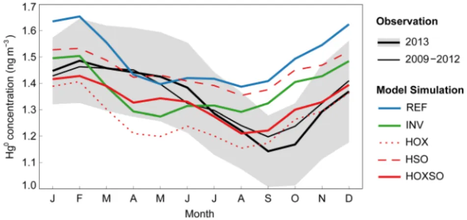
Figure 3 shows the average Hg0 concentration measured at the 11 NADP AMNet ground-based sites.
The average observation in 2013 is similar to that in 2009–2012, both of which indicate pronounced seasonal variations with a maximum of Hg0 in late winter and early spring (about 1.45 ng m-3 in February–April) and
a minimum in late summer and early fall (about 1.20 ng m-3 in August–October). We use the Normalized
Root Mean Square Error (NRMSE) to evaluate the performance of model simulations: NRMSE =
√
—————————
12 × ∑12 i = 1 (Hg0obs,i - Hg0mod,i)2 ∑12 i = 1 Hg0obs,i (2)Table 2. Observed and modeled Hg0 concentrations during NOMADSS
Over terrestrial surfaces Over oceanic surfaces Mann-Whitney
U test
Median ± MAD N. of samples Median ± MAD N. of samples
Background within-PBL NOMADSS observations
Hg0 (ng m-3) 1.45 ± 0.09 360 1.55 ± 0.11 73 p < 0.001 Isoprene (ppbv) 1.38 ± 0.49 358 0.00 ± 0.01 71 p < 0.001 DMS (pptv) 1.95 ± 1.63 176 8.26 ± 4.37 60 p < 0.001 REF Hg0 (ng m-3) 1.39 ± 0.03 360 1.32 ± 0.03 73 p < 0.001 INV Hg0 (ng m-3) 1.30 ± 0.03 360 1.28 ± 0.02 73 p = 0.45 HOXSO Hg0 (ng m-3) 1.29 ± 0.05 360 1.26 ± 0.05 73 p < 0.001 HOCEAN Hg0 (ng m-3) 1.29 ± 0.03 360 1.29 ± 0.05 73 p = 0.67 doi: 10.12952/journal.elementa.000100.t002
where Hg0
obs,i and Hg0mod,i are the observed and modeled Hg0 concentrations in the ith month, respectively.
A smaller NRMSE value indicates a better model performance. Compared to the average NADP AMNet observation in 2013, the NRMSE values for REF, INV, HOX, HSO, and HOXSO are 0.14, 0.09, 0.09, 0.10, and 0.05, respectively, and thus HOXSO has the best performance among them. As shown in Figure 3, HOXSO is also the only simulation that reproduces the observed seasonal pattern of Hg0 concentration. The
two changes applied in HOXSO, the faster summertime Hg0 oxidation (also made in HOX) and the elevated
springtime mid-latitude soil volatilization (also made in HSO), are both essential for modeling this seasonal pattern. The tripled summertime BrOx accelerates the conversion of Hg0 to HgII through oxidation, and thus
the modeled Hg0 concentration in HOXSO shows a similar decreasing gradient (about -0.06 ng m-3 month-1)
during the summer months with the observation in 2013 (about -0.08 ng m-3 month-1) and in 2009–2012
(about -0.04 ng m-3 month-1). However, the model simulations without enhanced oxidation (REF, INV, and
HSO) cannot reproduce this feature in the observed Hg0 concentration. In contrast, the simulations without
elevated soil volatilization (REF, INV, and HOX) show a large decline of about 0.23 ng m-3 in modeled Hg0
during the spring months, which is not seen in the ground-based observations. By increasing springtime soil volatilization, HOXSO better reproduces the observed Hg0 trend in this season. Since the two sensitivity
simulations, HOX and HSO, cannot reproduce the observed seasonal pattern of ground-based Hg0, hereafter
we do not compare their results with ship cruise and aircraft measurements. Figure S2 shows the comparison of HgII wet deposition fluxes between the MDN measurements and different model simulations (REF, INV,
and HOXSO) during 2013 summer over eastern North America. REF and INV have similar insignificant positive biases of +2% and +1%, respectively. This is because only Hg0 surface fluxes differ between these two
simulations. HOXSO shows a large positive bias of +59% due to the enhanced bromine radical fields used in this sensitivity simulation. It is noted that this bias should become smaller if an in-plume HgII reduction
is applied in GEOS-Chem (e.g., Zhang et al., 2012).
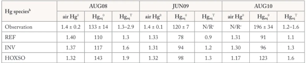
Table 3 compares the observed and modeled concentrations of Hg in both the atmospheric boundary layer and the ocean mixed layer for three summertime ship cruises in the Northwest Atlantic Ocean (Soerensen et al., 2013). These simulations (REF, INV, and HOXSO) produce air Hg0 concentrations (1.2–1.4 ng m-3) within
the uncertainty ranges of the observations. Among these simulations, REF leads to the lowest mixed layer concentrations of both Hgaq0 and HgaqT, whereas HOXSO predicts the highest. Compared with measurements,
REF and INV underestimate mixed layer Hgaq0 concentrations by 17–54% and 12–51%, respectively. HOXSO
models comparable Hgaq0 concentrations for one ship cruise (AUG08), but still underestimates its levels for
the other two (up to 40%). On average, HOXSO underestimates the observed mixed layer Hgaq0 by about
20%. As shown in Figure 4 (b–d), the modeled net oceanic Hg0 emission fluxes also follow the order of
REF < INV < HOXSO. Considering that HOXSO may underestimate mixed layer Hgaq0 concentrations
by 40% and that different gas exchange parameterizations may lead to a 30% variability in estimated oceanic Hg0 fluxes (Sunderland et al., 2010; Andersson et al., 2007), we conduct an additional sensitivity simulation
referred to as HOCEAN, in which the net Hg0 fluxes from the Northwest Atlantic (100–60° W, 15–45°
N) during the summer months (June–July–August) are increased by 80% above the oceanic Hg0 fluxes in
HOXSO. HOCEAN thus represents a potential upper limit of oceanic emissions from the Northwest Atlantic determined from the above model–observation comparison of ship cruises.
Table 2 shows the background within-PBL Hg0 observations during the NOMADSS aircraft campaign,
divided into two groups (over terrestrial and over oceanic surfaces), and the corresponding model results from REF, INV, HOXSO, and HOCEAN. All these model simulations predict lower Hg0 concentrations
than the DOHGS observed. The modeled median concentrations of Hg0 over terrestrial surfaces range from
1.29–1.39 ng m-3, about 4–11% lower than its observed median of 1.45 ng m-3. This difference generally falls
within the overall measurement uncertainty range of 6–10% of the DOHGS. In contrast, by comparing the observed and modeled Hg0 concentrations (1.33 and 1.30–1.42 ng m-3, respectively) during the NOMADSS
Figure 3
Averaged monthly observations and model simulations of Hg0
concentrations for the NADP AMNet ground-based sites.
Locations of the 11 remote/rural NADP AMNet sites are plotted in Figure 1. The thick black line and gray shaded region show the average and 1σ uncertainty range of observed Hg0 concentration in 2013. The thin black line shows the average observation in 2009– 2012. The blue, green, and red solid lines indicate model results from REF, INV, and HOXSO, respectively. The dotted and dashed red lines indicate model results from HOX and HSO, respectively.
period (2013 June–July) for the 11 AMNet ground-based sites in the eastern United States, we do not find a consistent negative bias in our model simulations (Figure 3). As described earlier, the DOHGS observed a significantly higher Hg0 concentration of 0.10 ng m-3 over oceanic surfaces in the Northwest Atlantic than
over terrestrial surfaces in the eastern United States. However, our model simulations cannot reproduce this land–ocean difference. As shown in Table 2, REF, INV, and HOXSO indicate that the median Hg0
concentrations over oceanic surfaces are 0.07 (p < 0.001), 0.02 (p = 0.45), and 0.03 (p < 0.001) ng m-3 lower
than those over terrestrial surfaces. HOCEAN increases the summertime net Hg0 flux from the Northwest
Atlantic by 80% than HOXSO, and predicts comparable (p = 0.67) Hg0 concentrations over terrestrial surfaces
(1.29 ± 0.03 ng m-3) and over oceanic surfaces (1.29 ± 0.05 ng m-3). Among our sensitivity GEOS-Chem
model simulations, HOCEAN can be considered as the best simulation with regard to the comparison with Hg0 observations.
Discussion
Enhanced terrestrial flux of Hg
0in spring
We have described that HOXSO can reproduce the seasonal variation of Hg0 concentration observed at
the NADP AMNet ground-based sites with an enhanced springtime soil volatilization in the mid-latitude region (20°–60°). As shown in Figure 2, the net terrestrial fluxes of Hg0 (the sum of soil volatilization, rapid
recycling, and dry deposition) modeled by HOXSO are positive in the spring months. We hypothesize that the mid-latitude terrestrial flux of Hg0 in spring may be enhanced based on the following evidence from both
atmospheric mercury modeling and surface flux measurements. Song et al. (2015) quantitatively constrained monthly soil volatilization using worldwide ground-based observations and a Bayesian inversion approach. As shown in Figure 2, the 1σ uncertainty range of soil volatilization from the emission inversion revealed an enhancement during the spring months (Song et al., 2015), and increasing the soil volatilization by a factor of 4 agrees well with this modeling result. The measured net Hg0 fluxes in the mid-latitudes for different land
use types (i.e., forest, grassland, agriculture, and bare soil) and different seasons are summarized in Table S1. We find that most of them (7 out of 9) show higher terrestrial Hg0 fluxes in spring (by 40% to a factor of
6) than the averages in other seasons. Bash and Miller (2007) suggested that springtime agricultural tilling operations can significantly mobilize Hg into the atmosphere from its soil pool. The small vegetation coverage in spring, which allows the penetration of solar radiation to the soil surface, may also be another important factor for the measured high Hg0 emission fluxes (Choi and Holsen, 2009). It is important to note, however,
that only limited terrestrial flux measurements are available and very large uncertainties exist in them. Net deposition fluxes of Hg0 during springtime have also been suggested (Mao et al., 2008; Converse et al., 2010).
Implications for regional terrestrial and oceanic Hg
0fluxes during summer
The NOMADSS aircraft campaign found higher Hg0 concentrations over the Northwest Atlantic than over
the eastern United States (Table 2). Gay et al. (2013) reported a similar finding by combining the NADP AMNet sites into several loosely defined groups, including a coastal/remote group (NS01 and NH06) and a continental/remote group (VT99, NY20, and GA40) (Figure 1). Three years of data show that the former group has about 0.07 ng m-3 higher Hg0 concentrations than the latter. However, the Hg0 measurement systematic
uncertainty for these NADP AMNet sites, which is estimated to be about 0.14 ng m-3 (10% of the observed
Hg0 concentration of 1.3–1.4 ng m-3; Figure 3), is larger than this 0.07 ng m-3 difference between the two site
groups, limiting our ability to apply these results in a modeling context. NOMADSS minimizes potential systematic differences since the DOHGS was used to measure Hg0 over both terrestrial and oceanic surfaces.
Table 3. Observed and modeled air and aqueous Hg for three summertime Northwest Atlantic ship cruisesa
Hg speciesb AUG08 JUN09 AUG10
air Hg0 Hg aq0 HgaqT air Hg0 Hgaq0 HgaqT air Hg0 Hgaq0 HgaqT Observation 1.4 ± 0.2 133 ± 14 1.3–2.9 1.4 ± 0.1 120 ± 7 N/Rc N/Rc 196 ± 34 1.2–1.6 REF 1.40 110 1.3 1.33 78 0.9 1.31 91 1.1 INV 1.37 117 1.6 1.31 94 1.2 1.30 96 1.3 HOXSO 1.32 143 1.9 1.32 98 1.3 1.17 123 1.6
a Observations are obtained from Soerensen et al. (2013). For the cruise in August 2008, we exclude aqueous mercury data measured in the coastal Gulf of Maine because they were affected by anomalously high freshwater inputs.
bThe units of air Hg0, Hg
aq0, and HgaqT are ng m-3, fM (10-12 mol m-3), and pM (10-9 mol m-3), respectively. cN/R, not reported.
This land–ocean difference of atmospheric Hg0 concentrations over eastern North America has important
implications for regional terrestrial and oceanic Hg0 fluxes. The modeled net surface fluxes in 100–60° W and
20–50° N during summer are shown in Figure 4 (b–d). Note that all model simulations also include the same three unidirectional sources that occur over land (i.e., anthropogenic, geogenic, and biomass burning), which together emit 3.1 Mg month-1 Hg0 from terrestrial surfaces (corresponding to an average Hg0 flux of 0.8
ng m-2 h-1), as shown in Figure 4a. REF emits an average net oceanic flux of 1.3 ng m-2 h-1 from the Northwest
Atlantic and an average net terrestrial flux of 0.8 ng m-2 h-1 from the eastern United States. (Figure 4b).
Thus, in REF, the total Hg0 flux emitted over land (1.6 ng m-2 h-1) is larger than that from oceanic surfaces
(1.3 ng m-2 h-1). As described earlier, in REF, the median Hg0 over land is 0.07 ng m-3 higher (p < 0.001)
than that over ocean, which is opposite to the observed land–ocean difference in NOMADSS. Among our model simulations, HOCEAN has the lowest terrestrial Hg0 flux of -0.6 ng m-2 h-1 (total Hg0 flux emitted
over land is thus 0.2 ng m-2 h-1) and the highest oceanic Hg0 flux of 3.3 ng m-2 h-1, and predicts the same Hg0
concentrations (p = 0.67) over both surfaces in NOMADSS. Consequently, the above comparison between our model results and NOMADSS observations implies either even higher oceanic Hg0 fluxes from the
Northwest Atlantic or lower Hg0 fluxes emitted from land in the eastern United States, or both, than the
fluxes simulated by HOCEAN.
We have demonstrated through the model–observation comparison of ship cruises that HOCEAN represents a potential upper limit of oceanic emissions from the Northwest Atlantic. However, riverine discharges of Hg, an oceanic source that is not considered in the 2D mixed layer slab ocean of GEOS-Chem, may lead to additional Hg0 emissions from coastal/shelf areas and help to reconcile the difference between
model results and NOMADSS observations. Soerensen et al. (2013) found, during the ship cruise AUG08 in the Northwest Atlantic (Figure 1), that enhanced freshwater inputs due to anomalously high precipitation in July 2008 strongly increased the mixed layer Hgaq0 concentrations and Hg0 fluxes in waters of the Gulf
of Maine approximately 60 km offshore (270 ± 50 fM and 7.2 ± 4.2 ng m-2 h-1), when compared to those in
more open waters (130 ± 14 fM and 3.8 ± 2.9 ng m-2 h-1). A spatial trend of higher Hg
aq0 levels in coastal
waters (∼ 100 km) than in open waters has also been observed in other cruises (e.g., Ci et al., 2011b). Two NOMADSS research flights, RF-14 and RF-16, sampled the oceanic air 50–150 km off the coast of South Carolina on July 5 and July 8 of 2013, respectively (Figure 1). Unusually high water discharges were measured in July 2013 for rivers in South Carolina (see Figure S3a for an example). Additionally, measurements within the NADP Mercury Deposition Network (MDN; Prestbo and Gay, 2009) showed heavy rainfall and high
Figure 4
Spatial distributions of modeled atmospheric Hg0 fluxes in eastern
North America in summer.
The average fluxes during the summer months (June–July– August) are shown. The sum of the three unidirectional emissions (anthropogenic, geogenic, and biomass burning) is shown in (a). The net terrestrial and oceanic fluxes from REF, INV, and HOXSO are plotted in (b), (c), and (d), respectively.
wet deposition fluxes of Hg in late June and early July 2013, right before the sampling time of these two flights (see Figure S3b for an example). Overall, these results suggest that riverine discharges of mercury may contribute to the observed high Hg0 concentration over the Northwest Atlantic.
HOCEAN simulates an average net terrestrial flux of -0.6 ng m-2 h-1, meaning that the simulated terrestrial
ecosystem in the eastern United States is a net sink of Hg0 during summer. The simulated dry deposition
of Hg0 of 2.0 ng m-2 h-1 is only partially offset by its evasion that includes soil volatilization (0.6 ng m-2 h-1)
and rapid recycling of newly deposited Hg (0.8 ng m-2 h-1). The global terrestrial flux measurement database
(Agnan et al., 2016) suggests a small positive median Hg0 flux of 0.1 ng m-2 h-1 (50% uncertainty range: -0.1
to 0.5 ng m-2 h-1) over background bare soil, which is in agreement with measured vertical profiles of Hg0
in soil pores (Obrist et al., 2014). However, forest is the most important land use type in the eastern United States, especially during summer when the leaf area index is maximum (thus leaf surface areas are several times larger than underlying soil surface areas) (Drummond and Loveland, 2010; Buermann et al., 2001). Forest canopies can reduce Hg0 evasion from underlying soils by absorbing most of the incoming solar radiation
and suppressing the rising of soil temperature (Wang et al., 2006; Choi and Holsen, 2009). Foliage is well-known to constitute a net sink of atmospheric Hg0 through stomatal and non-stomatal uptake (Wang et al.,
2014; Stamenkovic and Gustin, 2009), and the median Hg0 flux measured over leaves at background forest
sites is -0.12 ng m-2 h-1 with a 50% uncertainty range from -1.48 to 1.65 ng m-2 h-1 (Agnan et al., 2016). Hg
translocation from soil to leaves is unlikely to be significant (Fay and Gustin, 2007; Cui et al., 2014). Therefore, it is not unreasonable to consider the summertime terrestrial ecosystem in the eastern United States as a net sink of Hg0, given relatively low soil evasion and high foliage uptake. However, it is not possible to provide
an accurate estimate for the magnitude of this sink, since reliable flux measurements over forests are currently lacking, and the mechanism of Hg transport in plant/vegetation is not well understood (Agnan et al., 2016). The unidirectional sources over land (i.e., anthropogenic, geogenic, and biomass burning) are also uncertain and their fluxes may be higher or lower than the values applied in our model. However, their uncertainties are small compared to those associated with terrestrial and oceanic fluxes in the studied region. In summer, simulated geogenic activities and biomass burning emit little atmospheric Hg0 from the eastern United States
(< 0.1 ng m-2 h-1 on average), and thus the contributions of their uncertainties on Hg0 fluxes are insignificant
in this context. The NEI 2011 inventory used in our model has an average Hg0 flux of 0.7 ng m-2 h-1 in the
eastern United States. In general, anthropogenic emissions in North America are considered to be relatively well constrained (1σ error around ± 30%) (e.g., Pacyna et al., 2010; AMAP/UNEP, 2013). Although U.S. EPA will not release the NEI inventory in 2013 (the year in which NOMADSS took place), another estimate, the Toxics Release Inventory (TRI; U.S. EPA, 2015), shows that the magnitudes of estimated mercury emissions for 2011 and 2013 differ only slightly (< 2%).
Figure 5
Spatial distributions of modeled vertical exchange fluxes in the North Atlantic in summer.
Model results from HOXSO are shown. The plots in (a–e) indicate different mercury exchange fluxes between the atmosphere and the mixed layer and between the mixed layer and subsurface waters. The spatial distribution of precipitation rate is shown in (f) overlaid with geopotential height contour lines at 850 hPa. The geopotential height data are obtained from the NCEP/ NCAR reanalysis (http://www. esrl.noaa.gov/psd/data/gridded/ reanalysis/).
Origin of high Hg
0flux from the Northwest Atlantic
Based on the comparison between model results and aircraft and ship cruise observations, our analysis suggests a high Hg0 flux from the Northwest Atlantic. In our simulations, this high Hg0 flux helps to explain the
land–ocean differences of observed atmospheric Hg0 concentrations in the eastern North America, and also
agrees with the observed high aqueous Hg0 levels in the mixed layer. In contrast, a recent study by Weigelt et al.
(2015) classified Hg0 data observed at the Mace Head station on the Northeastern Atlantic coast of Ireland
into different air mass groups according to their geographical origins. Air masses originating mostly from the Northeast Atlantic were found to have generally lower Hg0 concentrations (0.07 ± 0.04 ng m-3 calculated
from monthly means and 0.04 ± 0.05 ng m-3 from monthly medians, both using data in 2010–2013) than
those from continental Europe. As shown in Figure S4, our model simulations of the Northwest Atlantic, particularly the waters near the continental United States, have overall higher Hg0 fluxes when compared
to the Northeast Atlantic. This is qualitatively consistent with the different land–ocean patterns of observed atmospheric Hg0 over the Northeast and Northwest Atlantic.
The model also enables us to identify physicochemical processes that lead to simulated high Hg0 fluxes in
the Northwest Atlantic (and the relatively low fluxes in the Northeast Atlantic). The modeled Hg0 fluxes are
positively correlated with the mixed layer Hgaq0 concentrations (Equation 1), which are in turn determined
by multiple processes in the mixed layer, including photochemical- and biological- redox reactions and adsorption/desorption on particles, and the vertical interactions of the mixed layer with the above atmosphere and subsurface waters. The wet/dry deposition of HgII from the atmosphere is a source of mercury in the
mixed layer, whereas Hg0 evasion into the atmosphere is a sink. Vertical exchanges between the mixed layer
and subsurface waters include entrainment/detrainment, wind-driven Ekman pumping, and particle sinking (biological carbon pump) (Soerensen et al., 2010; Batrakova et al., 2014; Song et al., 2015). Figure 5a shows the spatial distribution of net Hg0 fluxes (modeled by HOXSO) from the North Atlantic Ocean (100° W–20° E,
20–60° N) in summer. The spatial distributions of modeled Hg fluxes associated with several above-mentioned processes are shown in Figure 5(b–e). A comparison of the magnitude of these Hg fluxes indicates that the high wet deposition of HgII into the Northwest Atlantic is the dominant process determining the simulated
high net oceanic flux of Hg0 from this region. The wet deposition of HgII is closely related to the precipitation
rate, which also has a spatial pattern with generally higher values in the Northwest Atlantic, in particular the waters near the continental United States, and lower values in the Northeast Atlantic (see Figure 5f). The summertime precipitation in the North Atlantic is influenced by the North Atlantic Subtropical High (NASH, also known as the Bermuda High), a semi-permanent high pressure system in the lower troposphere (Li et al., 2012). As shown in Figure 5f, strong precipitation is located along the western boundary of the NASH, which can be represented by the 1560 m geopotential contour line at 850 hPa (Li et al., 2011), while the precipitation rate in eastern side of the NASH is very small. Overall, the high simulated Hg0 flux from
the Northwest Atlantic is mainly a result of high wet deposition of HgII, which is in turn linked to high
precipitation rates in this region during summer. Given the uncertainties in modeling oceanic mercury and the limited representation of these processes in our slab ocean model, however, our ability to draw process-based conclusions from this study is limited. Similarly, a more detailed 3D oceanic mercury model (Zhang et al., 2014) suggests that high wet deposition of HgII leads to high Hg0 flux from the Northwest Atlantic
(Zhang Y, personal communication).
Conclusions
Atmosphere–surface exchange of Hg0 in eastern North America is constrained by combining aircraft-based
observations made during the 2013 summer NOMADSS campaign (as well as ground- and ship-based measurements) and GEOS-Chem CTM simulations. As a consistent instrumentation (the DOHGS) measured Hg throughout NOMADSS, the systematic uncertainty of Hg0 concentration measurements at
different locations is minimized. Within the PBL, significantly higher median Hg0 concentrations were
observed over oceanic surfaces of the Northwest Atlantic than over terrestrial surfaces of the eastern United States during NOMADSS (p < 0.001). The model simulation (HOCEAN) with a low (negative) terrestrial Hg0 flux and a high (positive) oceanic flux in this region obtains the same Hg0 concentrations (p = 0.67)
over both surfaces. Riverine discharges of mercury, an oceanic source that is not included in GEOS-Chem but may be significant in the NOMADSS period, may help to reconcile the model–observation discrepancy. By analyzing processes in the 2D mixed layer slab ocean of GEOS-Chem, we show that inferred high Hg0
emission fluxes from the Northwest Atlantic may be a result of high wet deposition fluxes of oxidized mercury, which are in turn linked to high precipitation rates in this region. Given relatively low soil evasion and high foliage uptake, it is likely that terrestrial ecosystem in the summer eastern United States acts as a net sink of Hg0. Increasing simulated terrestrial fluxes of Hg0 in spring compared to other seasons can better reproduce
References
Agnan Y, Le Dantec T, Moore CW, Edwards GC, Obrist D. 2016. New constraints on terrestrial surface–atmosphere fluxes of gaseous elemental mercury using a global database. Environ Sci Technol 50(2): 507–524. doi:10.1021/acs.est.5b04013. AMAP/UNEP. 2013. Technical background report for the Global Mercury Assessment 2013. Arctic Monitoring and
Assessment Programme, Oslo, Norway/UNEP Chemicals Branch Geneva, Switzerland. http://www.amap.no/documents/
doc/technical-background-report-for-the-global-mercury-assessment-2013/848. Accessed February 2, 2016. Ambrose JL, Gratz LE, Jaffe DA, Campos T, Flocke FM, et al. 2015. Mercury emission ratios from coal-fired
power plants in the Southeastern United States during NOMADSS. Environ Sci Technol 49(17): 10389–10397. doi: 10.1021/acs.est.5b01755.
Ambrose JL, Lyman SN, Huang J, Gustin MS, Jaffe DA. 2013. Fast time resolution oxidized mercury measurements during the Reno Atmospheric Mercury Intercomparison Experiment (RAMIX). Environ Sci Technol 47(13): 7285–7294. doi: 10.1021/es303916v.
Amos HM, Jacob DJ, Kocman D, Horowitz HM, Zhang Y, et al. 2014. Global biogeochemical implications of mercury discharges from rivers and sediment burial. Environ Sci Technol 48(16): 9514–9522. doi: 10.1021/es502134t. Amos HM, Jacob DJ, Streets DG, Sunderland EM. 2013. Legacy impacts of all-time anthropogenic emissions on the
global mercury cycle. Global Biogeochem Cy 27(2): 410–421. doi: 10.1002/gbc.20040.
Andersson ME, Gårdfeldt K, Wängberg I, Sprovieri F, Pirrone N, et al. 2007. Seasonal and daily variation of mercury evasion at coastal and off shore sites from the Mediterranean Sea. Mar Chem 104(3–4): 214–226. doi:10.1016/j.marchem.2006.11.003.
Andersson ME, Gårdfeldt K, Wängberg I, Strömberg D. 2008. Determination of Henry’s law constant for elemental mercury. Chemosphere 73(4): 587–592. doi: 10.1016/j.chemosphere.2008.05.067.
Apel EC, Emmons LK, Karl T, Flocke F, Hills AJ, et al. 2010. Chemical evolution of volatile organic compounds in the outflow of the Mexico City Metropolitan area. Atmos Chem Phys 10(5): 2353–2375. doi: 10.5194/acp-10-2353-2010. Ariya PA, Amyot M, Dastoor A, Deeds D, Feinberg A, et al. 2015. Mercury physicochemical and biogeochemical
transformation in the atmosphere and at atmospheric interfaces: A review and future directions. Chem Rev 115(10): 3760–3802. doi: 10.1021/cr500667e.
Ariya PA, Khalizov A, Gidas A. 2002. Reactions of gaseous mercury with atomic and molecular halogens: Kinetics, product studies, and atmospheric implications. J Phys Chem A 106(32): 7310–7320. doi: 10.1021/jp020719o.
Bash JO, Miller DR. 2007. A note on elevated total gaseous mercury concentrations downwind from an agriculture field during tilling. Sci Total Environ 388(1–3): 379–388. doi: 10.1016/j.scitotenv.2007.07.012.
Batrakova N, Travnikov O, Rozovskaya O. 2014. Chemical and physical transformations of mercury in the ocean: A review.
Ocean Sci 10(6): 1047–1063. doi: 10.5194/os-10-1047-2014.
Buermann W, Dong J, Zeng X, Myneni RB, Dickinson RE. 2001. Evaluation of the utility of satellite-based vegetation leaf area index data for climate simulations. J Clim 14(17): 3536–3550. doi: 10.1175/1520-0442(2001)014<3536:eo tuos>2.0.co;2.
Chen HS, Wang ZF, Li J, Tang X, Ge BZ, et al. 2015. GNAQPMS-Hg v1.0, a global nested atmospheric mercury transport model: Model description, evaluation and application to trans-boundary transport of Chinese anthropogenic emissions.
Geosci Model Dev 8(9): 2857–2876. doi: 10.5194/gmd-8-2857-2015.
Cheng I, Zhang L, Mao H, Blanchard P, Tordon R, et al. 2014. Seasonal and diurnal patterns of speciated atmospheric mercury at a coastal-rural and a coastal-urban site. Atmos Environ 82(0): 193–205. doi: 10.1016/j.atmosenv.2013.10.016. Choi H-D, Holsen TM. 2009. Gaseous mercury fluxes from the forest floor of the Adirondacks. Environ Pollut 157(2):
592–600. doi: 10.1016/j.envpol.2008.08.020.
Ci ZJ, Zhang XS, Wang ZW. 2011a. Elemental mercury in coastal seawater of Yellow Sea, China: Temporal variation and air–sea exchange. Atmos Environ 45(1): 183–190. doi: 10.1016/j.atmosenv.2010.09.025.
Ci ZJ, Zhang XS, Wang ZW, Niu ZC, Diao XY, et al. 2011b. Distribution and air-sea exchange of mercury (Hg) in the Yellow Sea. Atmos Chem Phys 11(6): 2881–2892. doi: 10.5194/acp-11-2881-2011.
Converse AD, Riscassi AL, Scanlon TM. 2010. Seasonal variability in gaseous mercury fluxes measured in a high-elevation meadow. Atmos Environ 44(18): 2176–2185. doi: 10.1016/j.atmosenv.2010.03.024.
Corbitt ES, Jacob DJ, Holmes CD, Streets DG, Sunderland EM. 2011. Global source–receptor relationships for mercury deposition under present-day and 2050 emissions scenarios. Environ Sci Technol 45(24): 10477–10484. doi: 10.1021/ es202496y.
Cui L, Feng X, Lin C-J, Wang X, Meng B, et al. 2014. Accumulation and translocation of 198Hg in four crop species.
Environ Toxicol Chem 33(2): 334–340. doi: 10.1002/etc.2443.
Dastoor A, Ryzhkov A, Durnford D, Lehnherr I, Steffen A, et al. 2015. Atmospheric mercury in the Canadian Arctic. Part II: Insight from modeling. Sci Total Environ 509–510: 16–27. doi: 10.1016/j.scitotenv.2014.10.112.
De Simone F, Gencarelli CN, Hedgecock IM, Pirrone N. 2014. Global atmospheric cycle of mercury: A model study on the impact of oxidation mechanisms. Environ Sci Pollut R 21(6): 4110–4123. doi: 10.1007/s11356-013-2451-x. Driscoll CT, Mason RP, Chan HM, Jacob DJ, Pirrone N. 2013. Mercury as a global pollutant: Sources, pathways, and
effects. Environ Sci Technol 47(10): 4967–4983. doi: 10.1021/es305071v.
Drummond MA, Loveland TR. 2010. Land-use pressure and a transition to forest-cover loss in the eastern United States.
BioScience 60(4): 286–298. doi: 10.1525/bio.2010.60.4.7.
Ebinghaus R, Jennings SG, Schroeder WH, Berg T, Donaghy T, et al. 1999. International field intercomparison measurements of atmospheric mercury species at Mace Head, Ireland. Atmos Environ 33(18): 3063–3073. doi: 10.1016/S1352-2310(98)00119-8.
Environment Canada. 2013. The 2011 National Pollutant Release Inventory downloadable datasets [dataset]. http://www. ec.gc.ca/inrp-npri/. Accessed February 2, 2016.
Fay L, Gustin M. 2007. Assessing the influence of different atmospheric and soil mercury concentrations on foliar mercury concentrations in a controlled environment. Water Air Soil Pollut 181(1–4): 373–384. doi: 10.1007/s11270-006-9308-6.