HAL Id: tel-02162077
https://tel.archives-ouvertes.fr/tel-02162077
Submitted on 21 Jun 2019HAL is a multi-disciplinary open access archive for the deposit and dissemination of sci-entific research documents, whether they are pub-lished or not. The documents may come from teaching and research institutions in France or abroad, or from public or private research centers.
L’archive ouverte pluridisciplinaire HAL, est destinée au dépôt et à la diffusion de documents scientifiques de niveau recherche, publiés ou non, émanant des établissements d’enseignement et de recherche français ou étrangers, des laboratoires publics ou privés.
Multi-dimensional Teager-Kaiser signal processing for
improved characterization using white light
interferometry
Gianto Gianto
To cite this version:
Gianto Gianto. Multi-dimensional Teager-Kaiser signal processing for improved characterization using white light interferometry. Signal and Image Processing. Université de Strasbourg, 2018. English. �NNT : 2018STRAD026�. �tel-02162077�
UNIVERSITÉ DE STRASBOURG
ÉCOLE DOCTORALE MATHEMATIQUES, SCIENCES DE L'INFORMATION
ET DE L'INGENIEUR (MSII) – ED 269
LABORATOIRE DES SCIENCES DE L'INGENIEUR, DE
L'INFORMATIQUE ET DE L'IMAGERIE (ICUBE UMR 7357)
THÈSE
présentée par :Gianto GIANTO
soutenue le : 14 Septembre 2018pour obtenir le grade de :
Docteur de l’université de Strasbourg
Discipline/ Spécialité: SIAR-Traitement du signal et des images
Multi-dimensional Teager-Kaiser signal
processing for improved characterization
using white light interferometry
THÈSE dirigée par :Dr. MONTGOMERY Paul Directeur de recherche, CNRS, ICube (Strasbourg)
Encadrant :
Dr. SALZENSTEIN Fabien Maître de conférences, ICube (Strasbourg)
RAPPORTEURS :
Pr. CHONAVEL Thierry Professeur des Universités, IMT Atlantique (Brest)
Dr. SANDOZ Patrick Chargé de Recherche, CNRS, FEMTO-ST (Besançon)
AUTRES MEMBRES DU JURY :
Dr. BOUDRAA Abdel Maître de conférences, Ecole Naval IRENAV (Brest)
ii
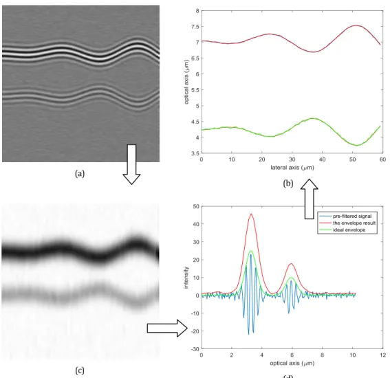
CONTENTS
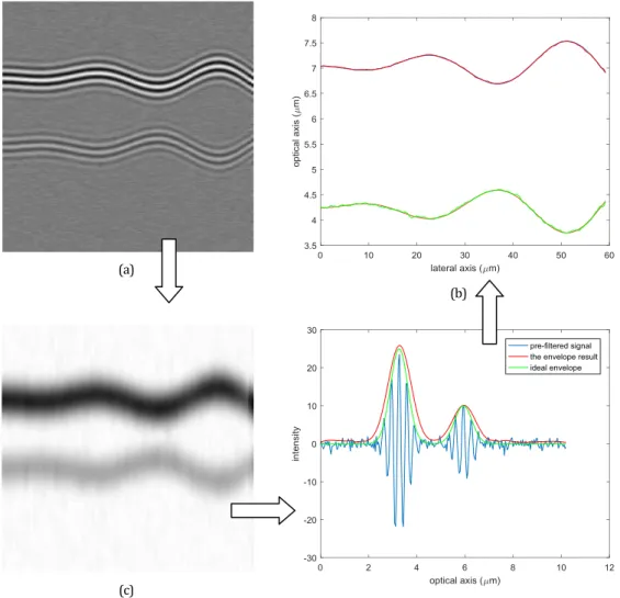
ACKNOWLEDGEMENTS ... vii
TABLE OF FIGURES ...viii
LIST OF TABLES ... xiv
RÉSUMÉ….. ... xv
NOMENCLATURE ... xviii
ABBREVIATIONS ... xix
GENERAL INTRODUCTION ... 1
Chapter 1. COHERENCE SCANNING INTERFEROMETRY ... 7
1.1 3D SURFACE PROFILING ... 7
1.2 GENERAL PRINCIPLE OF CSI ... 13
1.3 FRINGE SIGNAL ... 14
1.4 Z-SCAN TECHNIQUE (ID) ... 16
1.5 XZ-SCAN TECHNIQUE (2D) ... 16
1.6 ANALYSIS OF WHITE LIGHT INTERFERENCE FRINGES ... 17
1.6.1 Pre-filtering ... 18
1.6.2 Envelope Detection ... 18
1.6.3 Post-filtering ... 22
1.7 PERFORMANCE EVALUATION OF DIFFERENT OFFSET COMPONENT REMOVAL TECHNIQUES IN CSI... 23
1.7.1 The Offset Component removal technique ... 24
1.7.2 The denoising technique ... 27
1.7.3 Simulation results... 28
1.8 SURFACE MEASUREMENT ERRORS IN CSI ... 31
1.9 MICROSCOPE SYSTEM ... 33
1.10 STRUCTURE OF THE SAMPLES SURFACE ... 35
iii
1.11.1 Lateral resolution ... 38
1.11.2 Axial resolution ... 40
1.12 RÉSUMÉ DU CHAPITRE 1 ... 41
Chapter 2. COMPARISON OF PRE-FILTERING AND ENVELOPE DETECTION TECHNIQUES... 43
2.1 TEAGER KAISER ENERGY OPERATOR ... 43
2.1.1 Signal energy ... 43
2.1.2 Teager Kaiser Energy Operator ... 44
2.1.3 Discrete Teager Kaiser Energy Operator ... 45
2.1.4 Continuous Teager Kaiser Energy Operator ... 46
2.2 Performance Comparison Of Different Mother Wavelet In Continuous Wavelet Transform Algorithm On Fringe Signal Processing ... 47
2.2.1 Application wavelet analysis in fringe signal processing ... 47
2.2.2 Mother wavelet selection ... 47
2.2.3 Simulation results... 50
2.3 COMPARISON OF PRE-FILTERING TECHNIQUES ... 53
2.4 COMPARISON OF ENVELOPE DETECTION TECHNIQUES ... 55
2.4.1 Comparison Procedure ... 55
2.4.2 Synthetic Samples ... 56
2.4.3 Simulation Results ... 57
2.5 RESULTS USING MEASUREMENTS ON RESIN LAYER ON SILICON ... 64
2.6 CONCLUSION ... 72
2.7 RÉSUMÉ DU CHAPITRE 2 ... 72
Chapter 3. 2D FRINGE PROCESSING IN CSI ... 75
3.1 2D FRINGE ENVELOPE DETECTION ... 78
3.1.1 Analytic signal-Hilbert Transform (HT2D) ... 78
3.1.2 Teager Kaiser Energy Operator (TKEO2D) ... 79
3.2 THE ROBUSTNESS EVALUATION OF 2DTKEO AND 2DHT ... 81
3.3 DETECTION OF THE LAYERS NUMBER ON A TRANSPARENT LAYERS 84
iv
3.4 RESULTS OF MEASUREMENTS ON MYLAR POLYMER FILM USING
Z-SCAN AND XZ-Z-SCAN TECHNIQUE ... 91
3.4.1 Z-scan technique (1D Fringe Processing) results ... 92
3.4.2 XZ-scan technique (2D Fringe Processing) results ... 93
3.4.3 Measurement of thickness of Mylar polymer film ... 96
3.4.4 Error Approximation of Thickness Measurement of Mylar Film ... 98
3.5 CONCLUSION ... 100
3.6 RÉSUMÉ DU CHAPITRE 3 ... 100
Chapter 4. 3D FRINGE PROCESSING IN CSI ... 103
4.1 XYZ-SCAN TECHNIQUE (3D) ... 103
4.2 3D TEAGER KAISER ENERGY OPERATOR ... 104
4.2.1 Continuous 3D Teager Kaiser Energy Operator ... 107
4.2.2 Discrete 3D Teager Kaiser Energy Operator ... 109
4.3 PROCEDURE OF 3D FRINGE PROCESSING ... 112
4.4 PERFORMANCE COMPARISON OF ENVELOPE DETECTION USING 1D, 2D, 3D FRINGE PROCESSING ... 116
4.5 EVALUATION OF THE MEASUSUREMENT ACCURACY USING STEP HEIGHT STANDARD ... 122
4.6 PERFORMANCE OF 3D FRINGE PROCESSING ON DIFFERENT REAL SAMPLES ... 129
4.7 PERFORMANCE COMPARISON OF 3D FRINGE PROCESSING USING CONTINUOUS 3DTKEO AND DISCRETE 3DTKEO ... 133
4.8 CONCLUSION ... 139
4.9 RÉSUMÉ DU CHAPITRE 4 ... 139
GENERAL CONCLUSION ... 142
CONCLUSION GÉNÉRALE ... 144
LIST OF PUBLICATIONS AND COMMUNICATIONS... 146
SUPPLEMENTARY WORK ... 148
v
Appendix-2: Multi-scale roughness measurement of cementitious materials using window resizing analysis ... 153 BIBLIOGRAPHY ... 157
vi
vii
ACKNOWLEDGEMENTS
This PhD research would not have been possible without the help, the support, and the contribution of many people and institutions.
Firstly, I am very grateful to my supervisor (Directeur de thèse), Paul Montgomery, whom I greatly respect, for supervising my research work over the years. Many thanks for all the advice, the encouragement, the availability and the hours he spent for reading and correcting the manuscript. I am also very grateful to my co-supervisor (Encadrant), Fabien Salzenstein, for his great availability for discussion whenever I had a problem or a question about my PhD research. Many thanks also for the help, the encouragement, and the contribution for the improvement of the manuscript.
Thanks are given to Audrey Leong-Hoï and Husneni Mukhtar for providing the measurements on real samples and to Stéphane Perrin for useful discussions, all from the IPP team. Finally, I will always remember all of the kindness of my colleagues in the IPP team and to all parties that cannot be mentioned one by one for their support during my study.
My appreciation is also extended to the institution where I work, the Metrological Resources Development Centre, which gave me permission to study in France. I am also grateful to the Indonesian Government (Ministry of Trade), which provided the scholarship for my studies.
viii
TABLE
OF
FIGURES
Fig. 1 Schematic of the OCT system [17] ... 2
Fig. 2 Challenges of fringe signal processing in CSI ... 5
Fig. 3 Schematic of confocal microscope: showing the scanning (a) in the focal plane of the objective and (b) out of focus. (c) schematic of chromatic confocal microscopy [44] .. 8
Fig. 4 Phase determination, from 4 discrete steps of 120°[47]. ... 10
Fig. 5 The technique of the change of phase[47]. ... 10
Fig. 6 (a) A schematic layout of a CSI system (Leitz-Linnik interference microscope) and (b) typical signal from a single surface [49]. ... 13
Fig. 7 The interferogram construction on a surface using CSI (source: Guide to the measurement using CSI [50]). ... 14
Fig. 8 Double signal of white light interference fringes from a transparent layer (synthetic signal). ... 15
Fig. 9 Z scan technique. ... 16
Fig. 10 XZ scan technique [49]... 17
Fig. 11 The procedure of white light interference fringe analysis [53]. ... 17
Fig. 12 Fringe envelope detection process using Hilbert Transform technique [53]. ... 19
Fig. 13 FSA Algorithm ... 20
Fig. 14 The modulus of coefficient CWT of the fringe signal [53]. ... 22
Fig. 15 The use of post-filtering in CSI: (a) fringe signal, (b) prefiltered signal, and its envelope obtained (c) without post-filtering and (d) using post-filtering. ... 23
Fig. 16 An example of background variation on the fringe signal (resin on Si)... 24
Fig. 17 Illustration of the Savitzky Golay filter ... 27
Fig. 18 Synthetic fringe signals with: (a) constant, (b) linear, (c) non-linear offset components. ... 28
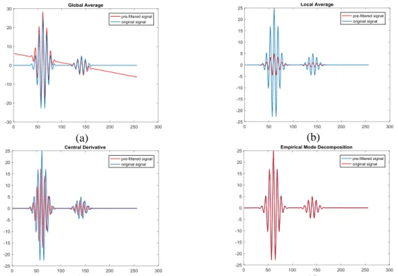
Fig. 19 Prefiltered signal obtained using: (a) Global average, (b) Local average, (c) Central derivative, (d) EMD, applied to the synthetic fringe signal with a constant offset component. ... 29
Fig. 20 Prefiltered signal obtained using: (a) Global average, (b) Local average, (c) Central derivative, (d) EMD, applied to the synthetic fringe signal with a linear offset component. ... 30
ix
Fig. 21 Prefiltered signal obtained using: (a) Global average, (b) Local average, (c) Central derivative, (d) EMD, applied to the synthetic fringe signal with a nonlinear offset component. ... 30 Fig. 22 A square wave grating that shows the batwing effect at the step edges ... 32 Fig. 23 Profile measurement of V-groove using white light interferometry [78] ... 33 Fig. 24 The modified Leica DMR-X interference microscope developed in the IPP team [83]. ... 35 Fig. 25 XZ images showing the interferograms from (a) a Step Height Standard and (b) a rock surface [85]. ... 36 Fig. 26 An XZ image showing the interferogram on a transparent layer on a substrate consisting of a resin layer on a silicon substrate ... 37 Fig. 27 An XZ image showing the interferogram of the transparent polymer film sample. ... 38 Fig. 28 The illustration of 3D PSF ... 40 Fig. 29 Wavelet familes: (a) Morlet, (b) complex Morlet, (c) Gaussian, (d) complex Gaussian, and (e) Mexican hat ... 48 Fig. 30 Synthetic fringe signal in (a) XZ image and (1D) ... 49 Fig. 31 Fringe envelope obtained using wavelet familes: (a) Morlet, (b) complex Morlet, (c) Gaussian, (d) complex Gaussian, and (e) Mexican hat ... 50 Fig. 32 Signal processing analysis for a wavy synthetic transparent surface: (a) output of pre-filtering using the EMD-SGolay filter; (b) surface profile, (c) 2D and (d) 1D fringe envelope obtained by CWT(complex Gaussian). ... 51 Fig. 33 Signal processing analysis for a wavy synthetic transparent surface: (a) output of pre-filtering using the EMD-SGolay filter; (b) surface profile, (c) 2D and (d) 1D fringe envelope obtained by CWT (complex Morlet). ... 52 Fig. 34 (a) Synthetic signal with noise σ =20% and prefiltered signal resulting from: (b) pre-filter 1; (c) pre-filter 2; (d) pre-filter 3. ... 54 Fig. 35 The comparison procedure to evaluate the performance of the different
algorithms[53]. ... 56 Fig. 36 Synthetic fringe signal with a non-linear offset and 10% Gaussian noise (XZ image) 256 x 256 pixel on a (a) flat transparent layer and (b) wavy transparent layer. .... 57 Fig. 37 Signal processing analysis for synthetic flat transparent surface: (a) output of pre-filtering using EMD-SGolay filter; (b) surface profile, (c) XZ image of envelope and (d) 1D fringe envelope obtained by TKEO. ... 58
x
Fig. 38 Signal processing analysis for a wavy synthetic transparent surface: (a) output of pre-filtering using EMD-SGolay filter; (b) surface profile, (c) XZ image of envelope and
(d) 1D fringe envelope obtained by TKEO... 59
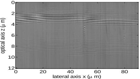
Fig. 39 Real fringe measurements on the resin on silicon sample: (a) raw XZ image data and (b) output of pre-filtering of (a) using the EMD-SGolay filter. ... 64
Fig. 40 2D envelope peak detection obtained by: (a) HT, (b) FSA, (c) CWT, (d) TKEO. 65 Fig. 41 Region of interest (ROI). ... 66
Fig. 42 1D fringe envelopes obtained by: (a) HT, (b) FSA, (c) CWT, and (d) TKEO at x = 11.41 µm near the resin edge where the two surfaces are closer together. ... 68
Fig. 43 Typical fringe signals from a sample of a resin layer on Silicon ... 69
Fig. 44 The dispersion curve corresponding to the resin layer ... 70
Fig. 45 The altitude Z (axis) of resin on Si ... 71
Fig. 46 The limitation of the PSM technique in height measurement ... 75
Fig. 47 The measurement of a spherical surface using the PSM technique resulting in phase discontinuities ... 76
Fig. 48 The technique of phase unwrapping in PSM to measure deeper structures ... 76
Fig. 49 The illustration of airy spot on the pixels ... 77
Fig. 50 The batwing effect on the measurement of a step ... 78
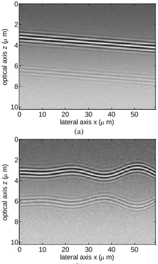
Fig. 51 (a) Synthetic XZ fringe image 256 x 256 pixel and (b) profile of fringe signal along the optical axis Z. ... 82
Fig. 52 Analysis of a noisy synthetic fringe signal (σ=20%): (a) 2D and (b) 1D fringe envelope obtained by Z-scan technique (FSA), (c) surface profile. ... 82
Fig. 53 Analysis of a noisy synthetic fringe signal (σ=20%): (a) 2D and (b) 1D fringe envelope obtained by XZ-scan technique (2DTKEO), (c) surface profile. ... 83
Fig. 54 Scheme of the interferogram construction on a transparent layer using CSI [83] 85 Fig. 55 Identify the number of Gaussian function using curve fitting ... 86
Fig. 56 (a) Synthetic XZ fringe image 256 x 256 pixel and (b) profile of fringe signal along the optical axis Z of transparent multilayer. ... 86
Fig. 57 Fringe envelope of a synthetic transparent layers ... 87
Fig. 58 (a) Surface detection on the synthetic transparent layers and (b) detected surface profile ... 88
Fig. 59 Comparison of the measured structures with the reference structures ... 89
Fig. 60 Interferogram of a transparent polymer film ... 90
xi
Fig. 62 Result of surface detection using the neighborhoods number as the threshold ... 91
Fig. 63 (a) XZ fringe image of a Mylar polymer and (b) the fringe signal along the optical axis Z. ... 91
Fig. 64 Logarithmic transformation of fringe envelope obtained by (a) FSA, (b) post-processing result using cubic spline smoothing. ... 92
Fig. 65 Surface extraction of Mylar polymer obtained by Z-scan technique using FSA algorithm. ... 93
Fig. 66 Logarithmic transformation of fringe envelope obtained by (a) 2DTKEO, (b) its post-processing result using cubic spline smoothing. ... 94
Fig. 67 Logarithmic transformation of fringe envelope obtained by (a) 2DHT, and (b) its post-processing result using cubic spline smoothing. ... 94
Fig. 68 Surface extraction of Mylar polymer obtained by XZ-scan technique using (a) 2DTKEO and (b) 2DHT. ... 95
Fig. 69 The refractive index of the Mylar ... 96
Fig. 70 Thickness measurements of Mylar polymer film. ... 98
Fig. 71 Thickness of Mylar polymer film. ... 98
Fig. 72 The technique of 3D fringe processing using 3DTKEO ... 103
Fig. 73 Stack image XYZ of fringe signals s(x,y,z) ... 104
Fig. 74 The stack image XYZ of fringe signal corresponds as reconstruction of the projection XZ slices and YZ slices ... 105
Fig. 75 The fringe envelope and the local frequency/orientation ... 106
Fig. 76 3D surface profile, XY surface profile z0(x,y), and the line surface profile ... 107
Fig. 77 Fringe signals of Graphene ... 112
Fig. 78 Pre-filtered fringe signals of Graphene after pre-processing step ... 113
Fig. 79 The volume of amplitude A(x,y,z) of fringe signals obtained using 3D fringe envelope detection ... 114
Fig. 80 Improvement results of 3D envelope detection using post-processing ... 115
Fig. 81 Surface extraction of a sample of Graphene obtained using 3D fringe signal processing ... 116
Fig. 82 Synthetic surface (XYZ image) 256 x 256 x 25 pixel and it’s fringe signals: (a), (c), (e) flat transparent layer and (b), (d), (f) wavy transparent layer. ... 117
Fig. 83 Signal processing analysis for synthetic flat transparent surface ... 118
xii
Fig. 85 Surface extracted obtained using: (a) and (b) Z-scan Technique (1DTKEO), (c) and (d) XZ-scan Technique (2DTKEO), (e) and (f) XYZ-scan Technique (3DTKEO). 120 Fig. 86 1D Fringe envelope obtained using (a) 1DTKEO, (b) 2DTKEO, (c) 3DTKEO . 121 Fig. 87 Camera image (XY slice) of the step-height standard (VLSI Standard Inc.) ... 122 Fig. 88 Fringe signal processing of Step Height Standards (SHS) by the modified Leitz-Linnik microscope ... 123 Fig. 89 Surface extracted of the Step Height Standards (SHS) obtained using 3D fringe signal processing on measurements from the modified Leitz-Linnik microscope ... 123 Fig. 90 Line profile of the Step Height Standards (SHS) obtained using 3D fringe signal processing on measurements with the modified Leitz-Linnik microscope ... 124 Fig. 91 Fringe signal processing of the Step Height Standards (SHS) from measurements on the new Fogale microscope ("Michelin") ... 124 Fig. 92 Surface extracted of the Step Height Standard (SHS) obtained using 3D fringe signal processing from measurements with the new Fogale microscope ("Michelin") ... 125 Fig. 93 Line profile of the Step Height Standards (SHS) obtained using 3D fringe signal processing from measurements with the new Fogale microscope ("Michelin") ... 125 Fig. 94 Fringe signal processing of the Step Height Standard (SHS) from measurements with the "immersion" Fogale microscope ... 126 Fig. 95 Surface extracted of the Step Height Standard (SHS) obtained using 3D fringe signal processing on measurements with the "immersion" Fogale microscope ... 126 Fig. 96 Line profile of the Step Height Standard (SHS) obtained using 3D fringe signal processing on measurements with the "immersion" Fogale microscope ... 127 Fig. 97 The measured step height obtained using: (a) Leitz-Linnik microscope; (b)
"Michelin" Fogale Microscope; (c) "immersion" Fogale microscope ... 128 Fig. 98 Fringe signals of DOE (Diffractive Optical Elements) ... 129 Fig. 99 Surface extraction of a sample of DOE (Diffractive Optical Elements) obtained using 3D fringe signal processing ... 129 Fig. 100 Fringe signals of Resin on Silicon ... 130 Fig. 101 (a) Surface extraction of a sample of Resin on Silicon obtained using 3D fringe signal processing and (b) the line profile ... 130 Fig. 102 Fringe signals from measurements on a Cable ... 131 Fig. 103 Surface extraction of a sample of Cable obtained using 3D fringe signal
processing ... 131 Fig. 104 Fringe signals of measurements on a Rock surface ... 132
xiii
Fig. 105 Surface extraction of a sample of Rock obtained using 3D fringe signal
processing ... 132 Fig. 106 (a) Fringe image of a Cable and (b) its fringe profile in 1D ... 133 Fig. 107 Prefiltered fringe image of a measurements from the Cable after the
pre-processing step and (b) its prefiltered fringe profile in 1D ... 134 Fig. 108 XZ fringe envelope obtained using (a) Continuous 3DTKEO and (b) Discrete 3DTKEO ... 135 Fig. 109 Comparison fringe envelope profile in 1D obtained using (a) Continuous
3DTKEO and (b) Discrete 3DTKEO ... 135 Fig. 110 3D Surface extraction obtained using (a) Continuous 3DTKEO and (b) Discrete 3DTKEO ... 136 Fig. 111 Image of surface profile obtained using (a) Continuous 3DTKEO and (b)
Discrete 3DTKEO ... 137 Fig. 112 Line profile comparison of Cable surface obtained using (a) Continuous
3DTKEO and (b) Discrete 3DTKEO ... 137 Fig. 113 Deviation value of surface extraction obtained using (a) Continuous 3DTKEO and (b) Discrete 3DTKEO ... 138 Fig. 114 Coordinate system used showing basic cell for δ = 1 (in this case giving 3x3 = 9 points) ... 153 Fig. 115 Measurement of surface roughness of unpolished samples using SCM and CSI ... 155 Fig. 116 Variation of different roughness values as a function of window size δdx for unpolished cement ... 156
xiv
LIST
OF
TABLES
Table 1 Computation times for the different pre-processing techniques applied to the synthetic fringe signals ... 31 Table 2 The lateral resolution criteria based on the illumination type ... 39 Table 3 Mean absolute error (mae) of surface extraction obtained using the CWT algorithm (complex Gaussian and complex Morlet wavelet) ... 53 Table 4 Experiment result using pre-filter 1 and different envelope detection
techniques (nm) ... 60 Table 5 Experiment result using pre-filter 2 and different envelope detection
techniques (nm) ... 61 Table 6 Experiment result using pre-filter 3 and different envelope detection
techniques (nm) ... 62 Table 7 Improvement of axial sensitivity of measurement obtained using Gaussian fitting (nm) ... 63 Table 8 Experiment result using pre-filter 3 and different envelope detection
techniques (nm) ... 67 Table 9 Mean absolute error (mae) of surface extraction corresponding to synthetic fringe image ... 84 Table 10 Mean value of mylar polymer thickness ... 97 Table 11 Performance Comparison of Envelope Detection using ... 121 Table 12 Calibration results of 3D fringe signal processing (3D TKEO) using Step Height Standards (SHS) ... 127
xv
RÉSUMÉ
L'utilisation de franges d'interférence en lumière blanche comme une sonde optique en microscopie interférométrique est d'une importance croissante dans la caractérisation des matériaux, la métrologie de surfaces et l'imagerie médicale. La technique, basée sur la microscopie interférométrique, a l’avantage d’y parvenir en ne faisant qu’un balayage vertical de l’échantillon, alors que les techniques de mesure ponctuelle nécessitent un grand nombre de balayages dans le plan horizontal pour imager un échantillon. L'Interférométrie en lumière blanche (Coherence Scanning Interferometry, CSI, également connu comme White Light Scanning Interferometry, WLSI) est une technique basée sur la détection de l’enveloppe de franges d’interférence. Cette technique (CSI) utilise généralement un échantillonnage des franges selon l'axe optique par moyen d'une acquisition d'une pile d'images XYZ. Le traitement d'image est ensuite utilisé pour identifier les enveloppes des franges, le long de l’axe Z à chaque pixel afin de mesurer les positions d’une surface unique ou des structures enterrées dans une couche. La mesure de la forme de la surface en CSI, nécessite généralement la détection d’un pic ou l'extraction de la phase du signal de franges mono-dimensionnel.
La plupart des méthodes sont basées sur un modèle de signal AM-FM, qui représente la variation de l'intensité lumineuse mesurée le long de l'axe optique d'un microscope interférométrique. Il a été démontré antérieurement, la capacité des approches 2D à rivaliser avec certaines méthodes classiques utilisées dans le domaine de l'interférométrie, en termes de robustesse et de temps de calcul. En outre, alors que la plupart des méthodes tiennent compte seulement des données 1D, il semblerait avantageux de prendre en compte le voisinage spatial utilisant des approches multidimensionnelles (2D, 3D), y compris le paramètre de temps afin d'améliorer les mesures.
Dans ce projet de recherche, nous sommes intéressés à développer de nouvelles approches n-D en utilisant Multi dimensionel Teager Kaiser qui sont appropriées pour une meilleure caractérisation des surfaces plus complexes et des couches transparentes. Dans ce travail, nous effectuons trois étapes pour le traitement des signaux de frange, à savoir le pré-traitement afin de supprimer le bruit et supprimer la composante de
xvi
décalage, la détection d'enveloppe et le post-traitement afin de déterminer plus précisément la mesure.
Nous commençons notre étude en évaluant la détection d'enveloppe en utilisant 1D Teager kaiser Energy Operator dans le traitement des signaux de frange, qui est comparé à d'autres techniques. Nous avons développé un programme de simulation de franges blanches (sur MATLAB) qui permet de comparer les résultats de mesures synthétiques (une couche transparente) effectués par différentes techniques de traitement de signal. Ces méthodes consistent en la Transformée de Fourier (TF), ondelettes, la FSA (Five-Sample-Adaptive), Opérateur d'énergie de Teager Kaiser (TKEO). Sur la base des résultats de simulation utilisant les images de franges synthétiques, il a été démontré que TKEO fournit les résultats les plus précis pour l'extraction de la surface supérieure et plus proche de la performance de CWT pour l'extraction de l'interface enterrée (surface arrière), mais présente l'avantage d'être plus compact et donc plus rapide. Les algorithmes TKEO et CWT fournissent également une meilleure extraction de surface que les algorithmes HT et FSA. Enfin, nous avons étudié la réalisation des algorithmes en utilisant des données réelles, c'est-à-dire l'image de frange de la couche de résine sur Silicium. Le résultat montre que CWT et TKEO ont des capacités différentes pour identifier deux positions de pic adjacentes. Sur la zone où se trouvent deux signaux de franges qui se chevauchent, le TKEO est capable d'obtenir l'enveloppe de frange qui distingue deux couches, tandis que CWT échoue dans le cas.
Après avoir commencé sur des signaux 1D, nous avons implémenté des traitements sur des signaux 2D. Dans ce projet de recherche, l'étude de la robustesse du traitement des franges 2D en CSI a également été réalisée pour la caractérisation d'un film de polymère Mylar transparent. Nous avons démontré la capacité des approches 2D Teager Kaiser à concurrencer certaines méthodes classiques (approches 1D) utilisées dans le domaine de l'interférométrie, en termes de robustesse. Ces résultats démontrent que l'enveloppe de frange XZ extraite par les approches 2D Teager Kaiser donne des résultats plus satisfaisants que l'approche 1D en révélant les structures internes et la surface arrière. La technique permet également une amélioration des détails dans les images XZ ainsi que des mesures plus précises de l'épaisseur du film polymère.
À la fin de ce travail, nous présentons l'étude de l'application de 3D Teager Kaiser Energy Operator (3DTKEO), qui est développé sur la base de l'opérateur d'énergie TK multi-dimensionnel. Grâce à une simulation utilisant un signal de frange synthétique,
xvii
nous avons évalué la robustesse des performances de 3DTKEO dans le traitement des signaux de franges, qui est comparé à l'approche 1D et 2D. De plus, nous avons également effectué l'algorithme sur des données réelles, c'est-à-dire une norme de hauteur de pas (VLSI Standard Inc.) afin d'évaluer la précision de la mesure. De plus, nous avons enrichi le domaine d'étude en testant l'algorithme sur différents échantillons, tels que le graphène, les DOE (Diffractive Optical Elements), la résine sur silicium, le câble et la roche.
xviii
NOMENCLATURE
, , Intensity signal at a given point of the sample surface (x,y)
Vertical scanning position along the optical axis in relation to the surface , , Offset intensity related to the reference and obje
s x y z z a x y z
0 ct beam intensities , Fringe contrastFringe envelope function
Mean wavelength of the light source
, Phase offset
( , ) Amplitude - value of the envelope for a single sampling position
( , ) Phase n b x y g z x y A x y x y
shift due to the scanning step ( , ) Intensities of sampling positions
First derivative of signal Second derivative of signal Teager Kaiser Energy Operator Instantaneous envelope n I x y s z s z s z s z s z a t t
Instantaneous phase, CWT coefficient function, where a is the scale factor and b is the shift factor Continuous function in time and frequency domain called the mother wavelet Total (or peak-vall
t W a b z R max min ey) roughness Highest peak of the surface profile Lowest peak of the surface profile Arithmetic roughness
mean line of the roughness profile height a j z z R z z
xix
ABBREVIATIONS
1D One dimensional
2D Two dimensional
2DHT Two dimensional analytic signal-Hilbert Transform
2DTKEO Two dimensional Teager-Kaiser energy operator
3D Three dimensional
AM-FM Amplitude Modulation - Frequency Modulation CSI Coherence Scanning Interferometry
CWT Continuous Wavelet Transform
DEOs Differential energy operators
EMD Empirical Mode Decomposition
ESA Energy Separation Algorithm
FF-OCT Full Field Optical Coherence Tomography
FFT Fast Fourier Transform
FSA Five-sample adaptive
FT Fourier Transform
HT Hilbert Transform
IMFs Intrinsic mode functions
MAE Mean absolute error
MEMS Micro Electro Mechanical Systems
NA Numerical Aperture OPD Optical path difference
PSM Phase Shifting Microscopy
xx SG filter Savitzky-Golay filter
SNR Signal to noise ratio
TK Teager-Kaiser
TKEO Teager-Kaiser energy operator
1
GENERAL
INTRODUCTION
This thesis is the result of my PhD research carried out for more than three years in fringe signal analysis in the field of Coherence Scanning Interferometry (CSI). The work has been performed in the IPP team (Photonics Instrumentation and Processes), in the ICube laboratory, University of Strasbourg-CNRS. The PhD scholarship has been funded by the Ministry of Trade, Indonesian government from 2014 to 2018. The purpose of the project was to develop new n-D approaches (2D, 3D) which are suitable for improved characterization of more complex surfaces and transparent layers using white light interferometry.
Several surface analysis techniques, such as the classical stylus probe, SEM (Scanning Electron Microscopy), AFM (Atomic Force Microscopy), confocal microscopy and interference microscopy, are important in the field of materials characterization, industrial metrology, and inspection [1],[2],[3]. It is often useful to use several techniques to elucidate the various surface characteristics, especially since there is no single technique capable of providing all the information on the morphology of a surface. The technique of interference microscopy, which makes use of light interference as the optical probe, has the advantages of being non-destructive and fast [4],[5],[6]. There are two families of techniques in interference microscopy: Phase Shifting Microscopy (PSM) and Coherence Scanning Interferometry (CSI). PSM is a mathematical method of fringe interpolation based on the introduction of known phase shifts between the two arms of the interferometer. The technique is well suited for the analysis of small surface roughness (depth < 200 nm) and commonly has a nanometric axial resolution. The dynamic range of PSM is limited to λ/2 due to the periodicity of the interference fringes that induce a 2π ambiguity in the measured surface profiles.
Due to this limitation, the second family of techniques, i.e. CSI was developed to allow the measurement of much deeper surfaces. The advantages of this technique compared to the PSM are the larger vertical depth of field and the possibility of measuring height differences of several microns and more [7],[8]. Nowadays, the use of CSI, which is also common known as white light interferometry, is widely used in various fields, including surface metrology, materials characterization, and medical imaging. For instance in the field of metrology, white light interferometry has been applied in the
2
characterisation of the fabrication of Micro Electro Mechanical Systems (MEMS) and other micro-component devices [9],[10],[11]. White light interferometry has also been applied for the measurement of surface roughness and microscopic structures in materials science and microelectronics [12],[13]. In another field, Dubois et al. developed full-field optical coherence tomography (FF-OCT) based on white light interferometry for high-resolution optical imaging of biological tissue [14],[15],[16]. This technique achieves a better spatial resolution than conventional OCT, without using an expensive light source, achieving a resolution of axial × transverse = 0.7 µm × 0.9 µm. Conventional OCT is usually based on a fibre Michelson interferometer illuminated by a broad-bandwidth spatially coherent source (laser). The measurement requires scanning of a point probe in the transverse direction over the sample in order to obtain the cross sectional image. The spatial resolution of OCT in the axial direction is defined by the coherence length of the illumination source, typically 10–15 µm in the case of a super luminescent diode (SLD) [16], [17], [18]. By using ultra-short femto second laser technology, the spatial resolution of OCT has improved down to ∼ 1 µm. Nowadays, OCT can be applied at the cellular level [14], [17].
A schematic layout of a simplified OCT system is illustrated in Fig. 1. The light from a low coherence source is coupled into a fiber-optic Michelson interferometer. This light is then split at a fiber coupler into the reference and the sample arm. The light retroreflected from the reference mirror and the light backscattered from the sample is recombined in the coupler and generates an interference pattern, which is detected by a single point detector (a photodiode) [17], [19], [20].
3
The use of white light interference fringes as an optical probe in microscopy has a long history. In 1665, Robert Hooke investigated the coloured fringe that can be observed in white light when the two glass plates are in contact [21]. This phenomenon can be called as the starting point of optical interferometry. Coloured fringe were then studied by Isaac Newton in 1717 as an interference pattern created by the reflection of light between two surfaces (known as “Newton’s rings”). Since then, the development of white light interferometry has been extended right up to the present day. The method developed for the three dimensional measurement of surface topography using white light interferometry is generally based on the analysis of fringe contrast. In this method, vertical fringe scanning (either the object or reference mirror) is carried out, followed by measuring the fringe intensity at each point of the object surface. The fringe pattern is observable when the optical path difference between the reference mirror position and the object surface is smaller than the coherence length of the used light. The zero value of the optical path difference is related to the surface position of the object (sample).
Developments in digital signal processing now allow three dimensional measurement using white light interferometry rapidly and automatically. The first automated 3D measurement using white light interferometry was reported by Balasubramanian in 1980 [22]. The variation in fringe contrast is recorded using a detector (CCD), point by point for each surface position. If the maximum fringe contrast level is observed, that point is determined as having a zero path difference that indicates the surface position. In 1987, Davidson reported the application of white light interferometry for integrated circuit inspection and metrology [23]. In this application, the use of an automated mechanical piezoelectric stage for fringe scanning was applied. The fringe intensity was captured using a detector, and then the peak of the fringe contrast was detected for profiling the object (integrated circuits). In 1990, by extending the concept of the Davidson’s work and focusing on the profilometry capabilities of white light interferometry, Lee and Starnd reported the advantage of white light interferometry over the conventional microscope in lateral resolution [24]. In 1992, the work on three dimensional sensing using white light interferometry for rough objects was reported [25]. In 1990, Chim and Kino introduced another way of fringe analysis by digital filtering of the interferogram (interference data). The fringe analysis used two different algorithms based on the Fourier Transform and Hilbert transform for extracting the fringe envelope [26], [27]. In 1993, Caber used the demodulation technique adapted from
4
communications theory for retrieving the fringe envelope [7], [28], [29]. In 1993, Montgomery and Fillard applied the algorithm of PFSM (peak fringe scanning microscopy) [30], [31], a very efficient algorithm which was then adapted for 3D measurement in real time [32],[33]. In 1996, Larkin developed the Five Sample Adaptive (FSA) algorithm which is an efficient algorithm in computational time for retrieving the fringe contrast envelope [34]. This was then demonstrated to be a member of the wider family of very compact and efficient Teager-Kaiser Energy Operators by Salzenstein et al. (TKEO) [35], [36], [37]. The work demonstrated that the TKEO algorithms are robust and very competitive with the other types of fringe envelope detection algorithms, being very efficient in terms of computation time, and making them quicker than the other techniques when implemented on the appropriate hardware. The extended versions of this operator show that the method substantially provides the effective results in term of the surface measurement [38]. Then, another method using the wavelet transform algorithm in order to retrieve the fringe envelope in white-light interferometry was applied by Sandoz in 1997 [39]. The advantage of the wavelet transform method implemented in white light interferometry is that it is very robust to noise.
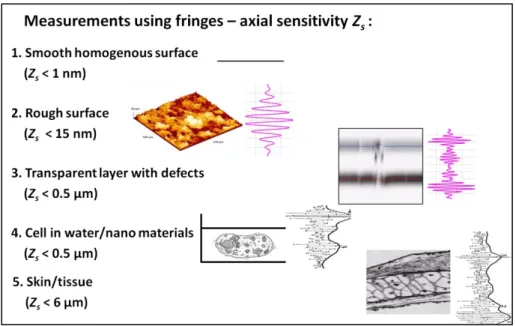
Most of the above fringe envelope detection methods are implemented on the one dimensional fringe signal (1D approach). The work in [13] used a 2D imaging processing method of the XZ images in an image stack for tomographic analysis of transparent layers. We also demonstrated in [12], [40] the ability of 2D approaches to compete with some classical methods used in the field of interferometry, in terms of robustness. Whereas most methods only take into account the 1D data, it is advantageous to take into account the spatial neighborhood using multidimensional approaches (2D, 3D). The objective of this project was therefore to study and develop new n-D approaches using Teager Kaiser energy operators for fringe analysis in CSI. This study is one part of dealing with several challenges of fringe signal processing currently in CSI. The challenges include the precision required along Z (optical axis) and XY (lateral direction), speed of processing, quantitative and qualitative aspects, noise aspects, the offset component, n-D approaches, and a formalised protocol for processing. Another challenge is the degree of complexity of the surface, that can be classified going from the simplest to the more complex, by a smooth homogenous surface, a rough surface, a transparent layer with defects, a cell in water, and skin/tissue, as shown in Fig. 2.
5
Fig. 2 Challenges of fringe signal processing in CSI
This thesis is composed of four main chapters.
The first chapter discusses the state of the art of Coherence Scanning Interferometry as related to this project. We mainly discuss the general principles of CSI and the procedure of fringe analysis. We study and observe the structure of the fringe signal and the various approaches (Z-scan and XZ-scan techniques) for fringe analysis. The study of pre-processing for the offset component removal, microscope system, and description of the samples which we use in the work are also reported.
In the second chapter, we begin our study by evaluating the performance of envelope detection using the 1D Teager Kaiser Energy Operator, which is compared to other techniques. These methods consist of the Fourier Transform (TF), wavelet, the FSA (Five-Sample-Adaptive). We have developed a simulation program (on MATLAB) that allows the comparison of the performance of different methods using a synthetic fringe signal (a synthetic transparent layer). Then, we have studied the realization of the algorithms using real data, in this case on fringe images from a resin layer on Silicon.
In the third chapter, we implement the 2D approach using Teager Kaiser for fringe analysis. In this work, the study of the robustness of the 2D approach in CSI was carried out for the characterization of a transparent polymer film. The results demonstrate that the XZ fringe envelope extracted by the 2D Teager Kaiser approaches gives more satisfactory results than the 1D approach by revealing the internal structures and the rear surface of
6
the transparent polymer film. The technique also results in improved details in the XZ images as well as more accurate measurements of the thickness of the polymer film.
In the fourth chapter, we present the study of the application of the 3D Teager Kaiser Energy Operator (3DTKEO), which is developed on the basis of the multi-dimensional Teager Kaiser energy operator. Through a simulation using a synthetic fringe signal, we have evaluated the robustness of the 3DTKEO's performance in fringe signal processing, which is compared to the 1D and 2D approaches. In addition, we have also used the algorithm on real data, in this case a step height standard (VLSI Standard Inc.) to evaluate the accuracy of the measurement. In addition, we have enriched the field of study by testing the algorithm on various other samples, such as graphene, DOE (Diffractive Optical Elements), resin on silicon, cable, and rock.
7
Chapter 1. COHERENCE
SCANNING
INTERFEROMETRY
In this chapter, we discuss several of the existing three dimensional surface profiling techniques, including Atomic Force Microscopy (AFM), confocal microscopy, and interference microscopy. Futhermore, we describe how the technique of Coherence Scanning Interferometry (CSI) generates an interferogram (fringe signal). We study and observe the structure of the fringe signal and the various approaches (Z-scan and XZ-scan techniques) for the fringe analysis. Then, we focus on the steps of the fringe analysis procedure which we perform in this work. The study of pre-processing for the offset component removal and determination of the surface structure of the sample which we use in the work are also reported.
1.1 3D SURFACE PROFILING
The measurement of 3D surface structures is an important field in materials characterization and industrial metrology. The existing techniques of 3D surface topography measurement consist of contact profilometers and optical profilometers. A stylus profiler is the oldest contact profiler, using a tactile probe to measure the surface profile [1], [2]. The technique works by moving the object surface in relation to the stylus tip and sensing the height variations of the stylus tip to determine the surface height profile. In the 1980’s, another type of scanning probe profilometer involving near field microsopy was developed [41]. The first mode was Scanning Probe Microscopy (SPM), based on electron tunnelling, that works by moving a fine tip in close proximity to the sample surface, to within several nm to a few angstroms depending on the technique. The Atomic Force Microscope (AFM) is the most popular SPM, using Van der Waal’s forces that can provide 3D images of surfaces generally at the nanometer scale. AFM is popular particularly for use in measuring non-conductive materials such as cells, bacteria, viruses and proteins [42], [43].
AFM has the advantages of nanometric resolution, but the images take in general several minutes to several tens of minutes or more to acquire. Optical profilers on the other hand have the advantage of allowing high speed surface profiling. The two most
8
common optical profilers are confocal microscope and white light interferometery (Coherence Scanning Interferometry).
Confocal microscope. The confocal microscope is based on focusing principle, as
illustrated in Fig. 3. that uses a pinhole to ensure only light at the point of focus on the sample surface can enter the detector. Fig. 3(a) shows the sample in the focal plane of the objective, while the sample moving out of the focus is shown in Fig. 3(b). The complete image is formed through point by point scanning of the illuminating and detecting pinhole on the spot over the sample surface. The image will not be formed if the sample moves out of focus, as shown in Fig. 3(b).
Another type, the chromatic confocal microscope was then developed which the vertical scanning is not required [1],[4], as shown in Fig. 3(c). Rather than using the vertical scanning, the technique uses an objective with an axial chromatic aberration that has a different focus position for each different wavelength corresponding to the height of the surface. A spectrometer in place of CCD as a detector, detects the wavelength value. The measurement of the object focus position based on the spectrum measurement makes the measurement process much faster. The technique has the disadvantage of the optical sensitivity for the inhomogeneous materials. Similarly as the conventional confocal system, another disadvantage is the necessity of lateral scanning of the sample.
Fig. 3 Schematic of confocal microscope: showing the scanning (a) in the focal plane of the objective and (b) out of focus. (c) schematic of chromatic confocal microscopy [44]
pinhole Illuminating beam Focal plane Sample out of focus pinhole Illuminating beam Focal plane (a) (b) Spectrometer Object surface Object scan x y Spatial filter Spatial filter White light source
�
9
Phase Shifting Microscopy. There are two main techniques used in interference
microscopy: Phase Shifting Microscopy (PSM) and CSI [12],[8],[45]. PSM is a mathematical method of fringe interpolation based on the introduction of known phase shifts between the two arms of the interferometer. These phase shifts vary the optical path difference (OPD) which result in several interferograms. The technique is well suited for the analysis of small surface roughness (depth < 200 nm) and commonly has a nanometric axial resolution. The PSM also has the capability to deliver results with low noise and high precision for smooth optical surfaces. However, the dynamic range of PSM is limited to λ/2 due to the periodicity of the interference fringes that induce a 2π ambiguity in the measured surface profiles. Due to this limitation, the second family of techniques, i.e. CSI was developed to allow the measurement of much deeper surfaces. The advantages of this technique compared to the PSM are the larger vertical depth of field and the possibility of measuring height differences of several microns and more [7],[8].
In PSM technique, a monochromatic or quasi-monochromatic light source is used for illumination on the sample such as with Köhler illumination. During the measurement, the optical path difference (OPD) is changed by taking three or more images using the camera. The phase of the interference signal is then analyzed at each point on the image using the PSM algorithm. The altitude which represents the surface profile is calculated based on the result of the phase measurement.
The following Eq.(1.1) [46] express the intensity at a coordinate point (x,y) in an interference pattern:
(1.1)
where Io(x,y) is the irradiance, γ0 is the fringe visibility (also called modulation or
contrast), φ(x,y) is the signal phase, and αi is the phase shift. Based on the Eq. (1.1)
mathematically, the three unknown parameters: Io(x,y), γ0 and φ(x,y) can be calculated by
using at least three interferograms. The precision of the measurement in PSM technique can be improved using higher numbers of interferograms.
In order to introduce the phase shifts in PSM, there are two basic modes, i.e. the discrete mode and continuous mode. For description of this phase shift in discrete and continuous mode, the algorithm of 4 steps of 120° is chosen as illustration.
10
Discrete mode. The discrete mode of this technique based on the discrete phase steps calculation is also known as the phase stepping microscopy. The illustration in Fig. 4 shows a phase determination from 4 discrete mode which is represented by the intensity of the interference fringes. The phase is then can be calculated using the following equation, which is usually displayed as a grayscale image of the phase:
(1.2)
Fig. 4 Phase determination, from 4 discrete steps of 120°[47].
Continuous mode. The continuous mode of the phase change technique in PSM, also known as the technique of the phase integration. As illustrated in Fig. 5, the technique is based on a linear variation of the phase. The parameter T is the period time of the change of the phase, while the parameter τ, which depends on the number of interferograms, is a time of the acquisition of an image.
11
In this technique several interferograms over the period T (assuming T is continuous) are recorded in order to determine the initial phase. On the other hand, one interferogram represents each integration time τ. Fig. 5 shows the illustration of phase determination in continuous mode corresponding to the example of Fig. 4. The integration time represents respectively the phase determination of 4 steps of 120°.
PSM algorithms
Several phase reconstruction algorithms have been developed. The phase measurement algorithms are based on the acquisition of a series of N interferograms (N ranging generally from 3 to 7) obtained with known phase shifts. The essential parameters in these measurement techniques are the mode of variation of the phase (discrete or continuous), the frequency of acquisition of the interference fringes and the number N of interferograms used to calculate the phase at a given instant.
a. Three step technique
If a phase shift of 2π is introduced between the object and reference beams, the phase φ(x,y) can be deduced from the intensities I1, I2, I3 of the three interferograms recorded for
the angular offsets π/4, 3π/4, 5π/4. The intensities measured are given by:
1 0 2 0 3 0 , , 1 cos ( , ) 4 3 , , 1 cos ( , ) 4 5 , , 1 cos ( , ) 4 I x y I x y x y I x y I x y x y I x y I x y x y (1.3)The resolution of these equations gives the expressions of phase and visibility at a point of coordinates (x,y) as follows:
3 2 1 2 2 2 1 2 2 3 0 , , ( , ) , , , , , , , 2 , I x y I x y x y arctg I x y I x y I x y I x y I x y I x y x y I x y (1.4)12 b. Four step technique
The intensity of the interference fringes for phase shifts of 2π is given by:
1 0 2 0 3 0 4 0 , , 1 cos ( , ) , , 1 cos ( , ) 2 , , 1 cos ( , ) 3 , , 1 cos ( , ) 2 I x y I x y x y I x y I x y x y I x y I x y x y I x y I x y x y (1.5)By a combination of these equations, the phase and visibility can be calculated with the following expressions:
4 2 1 3 2 2 4 2 1 3 0 , , ( , ) , , , , , , , 2 , I x y I x y x y arctg I x y I x y I x y I x y I x y I x y x y I x y (1.6)c. Five step technique
The intensity of the interference fringes for phase shifts of 2π is given by:
1 0 2 0 3 0 4 0 5 0 , , 1 cos ( , ) , , 1 cos ( , ) 2 , , 1 cos ( , ) , , 1 cos ( , ) 2 , , 1 cos ( , ) I x y I x y x y I x y I x y x y I x y I x y x y I x y I x y x y I x y I x y x y 1.7)By a combination of these equations, the phase and visibility can be calculated by the following expressions:
2 4 3 5 1 2 2 2 4 3 5 1 0 2 , , ( , ) 2 , , , 2 , , 2 , , , , 4 , I x y I x y x y arctg I x y I x y I x y I x y I x y I x y I x y I x y x y I x y (1.8)13
As mentioned previously, the limited depth range of PSM led to the development of white light interferometry and a different technique altogether based on the fringe envelope detection to give unambiguous depth measurement over large depths. This is now presented in the next section.
1.2 GENERAL PRINCIPLE OF CSI
A typical layout of a CSI system is shown in Fig. 6(a) [11]. The working principle of the CSI technique is based on the cross coherence analysis between the reference beam and the reflected object beam which come from a low coherence source using a beam splitter. During the measurement of the sample surface, the reference beam is reflected from the reference mirror, whilst the reflected object beam is reflected from the sample [48].
(a)
(b)
Fig. 6 (a) A schematic layout of a CSI system (Leitz-Linnik interference microscope) and (b) typical signal from a single surface [49].
The two light beams are then combined at the detector. The interference will occur when the optical path difference between the reference beam and the reflected object beam is close to zero. This is when the optical path length to the sample is nearly identical with the optical path length to the reference mirror. With the goal of finding the interference maximum, fringe scanning is carried out at each point on the sample surface, point by point. The fringe intensities, which vary according to the change in distance between the sample and the objective (in z axis), are captured by the detector (camera) generating the stored data signal, or interferogram. Fringe analysis is then applied in order to retrieve the peak of the fringe contrast envelope which indicates the axial position of
14
the surface of the sample. Fig. 7 shows how the interference is constructed at each pixel, point by point in the detector (camera).
Fig. 7 The interferogram construction on a surface using CSI (source: Guide to the measurement using CSI [50]).
The advantage of white light over monochromatic light is its ability to avoid ambiguity in order to determine the fringe order due to white light having a low coherence length. On the other hand, many factors can affect the accuracy of the CSI measurements, including the camera performance, the control and linearity of the piezo-controlled vertical scanning, the metrology frame design, the environment, and the sample stability [50].
1.3 FRINGE SIGNAL
The light intensity giving rise to the fringe signal, s(x,y,z), captured from a detector (CCD) as the optical path difference is varied through focus in a white light interferometer, has the following form [26], [34]:
0
0
0 4 , , , , , , .cos , , where s x y z a x y z b x y g z z x y z z x y x y z k (1.9) The function s corresponds to the intensity signal at a given point of the sample surface (x,y), where z represents a vertical scanning position in relation to the surface. The parameter z is referred to as k, with k the index-scanning step and the value of scanning step. The height of the surface z0(x,y) is a spatial function that depends on lateral15
coordinates x and y. The quantity a(x,y,z) is an offset intensity related to the reference and object beam intensities, b(x,y) is the fringe contrast, g(z) is the fringe envelope function related to the spectral profile of the white light source, and λ0 is the mean wavelength of
the light source. The phase offset related to the phase change on reflection is represented by α(x,y). The fringe signal in Fig. 6(b) shows a synthetic fringe signal from a single surface that has been generated based on the structure of white light interferences in Eq.(1.9).
Fig. 8 Double signal of white light interference fringes from a transparent layer (synthetic signal).
Eq.(1.9) corresponds to the simple case of light propagation in air which is assumed to be equal to 1. In the case of the light passing through a transparent layer, a double signal is produced, one from each side of the layer (Fig. 8). In this case the refractive index is greater than one and wavelength dependent, thus inducing the phenomenon of dispersion for the signal from the other side of the layer. In this case the actual distance for the second signal is measured by Eq.(1.10). CSI measures the optical path difference along the optical axis Z. By measuring the distance separating the peaks of the two envelopes, the actual distance d of the transparent layer at that point (X,Y) can be measured. If the sample displacement d along the optical axis (Z) and the refractive index n of the layer is known, the actual distance d is:
d
n (1.10) A completely description about this topic will be discussed in Chapter 2 and Chapter 3 in measurement the sample of resin on Si and Mylar polymer film.
16
1.4 Z-SCAN TECHNIQUE (ID)
The description of fringe analysis in CSI using the Z-scan technique is shown in Fig. 9. By means of a single vertical scan of the sample, a stack of XYZ images is generated. Signal processing is then used to obtain the fringe envelopes along Z in order to measure the positions of the peak of the fringe envelope which corresponds to the height of the surface at each pixel in the XY image [51], [52].
Fig. 9 Z scan technique.
Z-scan technique allows the initial manual investigation of the nature and quality of the fringe signal obtained which is generated by CSI. A priori information of the nature of the fringe signal is useful for the checking the presence of artefacts, for instance in a complex layer.
1.5 XZ-SCAN TECHNIQUE (2D)
Two dimensional fringe signal processing can be chosen using the raw XYZ data by operating on the XZY images as shown in Fig. 10. The technique is based on analyzing the XZ fringe images at a given point along the Y axis. The fringes are low pass filtered in 2D so as to find the fringe envelope. By processing a given XZ image, the cross sectional profile of a transparent sample can be obtained [52], also known as a B-scan in optical coherence tomography.
17
Fig. 10 XZ scan technique [49].
1.6 ANALYSIS OF WHITE LIGHT INTERFERENCE FRINGES
In general, the techniques of signal processing developed in this work consist of three main steps: pre-filtering, envelope detection and post-filtering (Fig. 11). The envelope detection is needed in order to obtain the fringe envelope of which the peak represents the surface position. Pre-filtering is used to remove the offset component and reduce the noise, while post-filtering is used to determine more precisely the measurement.18
1.6.1 Pre-filtering
The robustness of the signal processing of fringe signals depends on the sensitivity to the different sources of signal noise and artifacts. Another problem lies in an additive offset component (background) which can appear in the fringe signals during the acquisition process, particularly over large scanning depths. In order to remove this offset component and the additive noise, it is important to filter out both of them before applying fringe envelope detection.
1.6.2 Envelope Detection
In the following we present the different techniques used to retrieve the fringe envelope in CSI.
1. Analytic Signal (Hilbert Transform)
In analytic signals, the Hilbert Transform is often used for the purpose of amplitude demodulation. If we consider a real signal s(t), then the analytic signal sA(t) is defined
as:
exp
A H
s t s t is t A t i t
(1.11) Where the Hilbert transform of a signal is given by:
1 1
H s u s t s t du t t u
(1.12) In the frequency domain, the analytic signal corresponds to:
1
A
S sign S (1.13) In particular, for obtaining the analytic signal sA(t), the negative frequency component
of the signal is suppressed, which can be performed using a Fast Fourier Transform (FFT). The main steps of the Analytic Signal (Hilbert Transform) technique using a Fast Fourier Transform (FFT) calculation are outlined in Fig. 12. The FFT is applied to the signal in Fig. 12(a), producing the spectrum of the signal (Fig. 12(b)). The FFT coefficients that correspond to negative frequencies are then replaced with zeros (Fig. 12(c)). Finally, the fringe envelope is extracted (Fig. 12(d)) by calculating the inverse FFT of the positive frequency packet in Fig. 12(c). By removing negative frequencies from the spectrum of real signal s(t), the signal provided by inverse FFT becomes
19
complex as shown in Eq. (1.11), which gives directly the phase (t) and the amplitude A(t).
(a) (b)
(c) (d)
Fig. 12 Fringe envelope detection process using Hilbert Transform technique [53].
2. Five Sample Adaptive (FSA) algorithm
The FSA technique is a fast and simple algorithm which has been commonly used in CSI to retrieve the fringe envelope [34]. The main idea of the technique is the application of phase shifting algorithms for white light interferogram demodulation and to use the fringe visibility (or modulation) to calculate the fringe envelope. In the case of the FSA technique, five interferograms are captured by a digital imaging system.
At each pixel location in the image (x,y), the value of the visibility(x,y) of the fringes at that point is calculated from the intensities of five sampling positions, In–2 to
In+2, along the optical axis z (Fig. 13):
2
2 2 4 1 3 5 1 ( , ) 4 2 4 A x y I I I I I (1.14) where I1 to I5 are the interferogram intensities, giving exact values when the phaseshifting between interferograms is 90. The amplitude A(x,y) can be calculated with
0 2 4 6 8 10 12 -5 0 5 optical axis (m) in te n si ty -150 -10 -5 0 5 10 15 20 40 60 80 100 frequency (106) m a g n it u d e -150 -10 -5 0 5 10 15 50 100 150 200 frequency (106) m a g n it u d e 0 2 4 6 8 10 12 -5 0 5 optical axis (m) in te n si ty
20
just two multiplications and one square root operation, which gives the advantage of efficient computation time. This well-known technique in fact corresponds to a derivative of the signal followed by the discrete Teager Kaiser operator which we discuss next.
Fig. 13 FSA Algorithm
3. Teager Kaiser Energy Operator (TKEO)
The Teager Kaiser Energy Operator (TKEO) [54] is an operator that tracks the instantaneous energy of a signal. This non-linear energy operator and its 1D/2D discrete versions has found applications in various fields of signal and image processing due to its success in analysing and demodulating AM-FM signals with high resolution, simplicity, and efficiency [55]. In its discrete version, only three samples are required at each time instant. In the continuous case, the Teager Kaiser Energy Operator is defined by:
2
2
2
2 s z s z s z s z s z s z s z z z
(1.15)where s(z) is the signal, s(z) and s(z) means the first derivative and the second derivative of s respectively. A discrete forward and backward approximation of the derivatives of Eq.(1.15) leads to the discrete TKEO [56]:
2
1 1
s n s n s n s n
![Fig. 14 The modulus of coefficient CWT of the fringe signal [53].](https://thumb-eu.123doks.com/thumbv2/123doknet/14459503.520222/43.892.221.706.183.617/fig-modulus-coefficient-cwt-fringe-signal.webp)
![Fig. 24 The modified Leica DMR-X interference microscope developed in the IPP team [83]](https://thumb-eu.123doks.com/thumbv2/123doknet/14459503.520222/56.892.204.716.104.490/fig-modified-leica-dmr-interference-microscope-developed-ipp.webp)