Minimum Eccentricity Shortest Path Problem: an Approximation Algorithm and Relation with the k-Laminarity Problem

HAL Id: hal-01366782

https://hal.archives-ouvertes.fr/hal-01366782

Preprint submitted on 15 Sep 2016

HAL is a multi-disciplinary open access

archive for the deposit and dissemination of

sci-entific research documents, whether they are

pub-lished or not. The documents may come from

teaching and research institutions in France or

abroad, or from public or private research centers.

L’archive ouverte pluridisciplinaire HAL, est

destinée au dépôt et à la diffusion de documents

scientifiques de niveau recherche, publiés ou non,

émanant des établissements d’enseignement et de

recherche français ou étrangers, des laboratoires

publics ou privés.

Minimum Eccentricity Shortest Path Problem: an

Approximation Algorithm and Relation with the

k-Laminarity Problem

Etienne Birmelé, Fabien de Montgolfier, Léo Planche

To cite this version:

Etienne Birmelé, Fabien de Montgolfier, Léo Planche. Minimum Eccentricity Shortest Path Problem:

an Approximation Algorithm and Relation with the k-Laminarity Problem. 2016. �hal-01366782�

Minimum Eccentricity Shortest Path Problem:

an Approximation Algorithm and

Relation with the k-Laminarity Problem

´

Etienne Birmel´e1_{, Fabien de Montgolfier}2_{, and L´eo Planche}1,2

1

MAP5, UMR CNRS 8145, Univ. Sorbonne Paris Cit´e etienne.birmele@parisdescartes.fr

2

IRIF, UMR CRNS 8243, Univ. Sorbonne Paris Cit´e

fm@liafa.univ-paris-diderot.fr leo planche@liafa.univ-paris-diderot.fr

Abstract. The Minimum Eccentricity Shortest Path (MESP) Problem consists in determining a shortest path (a path whose length is the dis-tance between its extremities) of minimum eccentricity in a graph. It was introduced by Dragan and Leitert [9] who described a linear-time algorithm which is an 8-approximation of the problem. In this paper, we study deeper the double-BFS procedure used in that algorithm and ex-tend it to obtain a linear-time 3-approximation algorithm. We moreover study the link between the MESP problem and the notion of laminarity, introduced by V¨olkel et al [12], corresponding to its restriction to a di-ameter (i.e. a shortest path of maximum length), and show tight bounds between MESP and laminarity parameters.

Keywords: Graph search, Graph theory, Eccentricity, Diameter, BFS, Approximation Algorithms, k-Laminar Graph

1

Introduction

For both graph classification purposes and applications, it is an important issue to determine to which extent a graph can be summarized by a path. Different path constructions and metrics to characterize how far the graph is from the constructed path can be used, for example path-decompositions and path-width [11] or path-distance-decompositions and path-distance-width [13]. Another ap-proach, on which we focus in this article, is to characterize the graph by a spine defined by one of its paths.

This problem was first studied in terms of domination, that is finding a path such that every vertex in the graph belongs to or has a neighbor in the path. Several graphs classes were defined in terms of dominating paths. [7] studies the graphs for which the dominating path is a diameter. [8] introduces dominating pairs, that is vertices such that every path linking them is dominating. Graphs such that short dominating paths are present in all induced subgraphs are char-acterized in [2]. Linear-time algorithms to find dominating paths or dominating vertex pairs were also developed for AT-free graphs [4, 6].

Dominating paths do not exist however in every graph and have no associated metric to measure the distance from the graph to the path. A natural extension of the notion of domination is the notion of k-coverage for a given integer k, defined by the fact that a path k-covers the graphs if every vertex is at distance at most k from the path. The smallest k such that a path k-covers the graph is then a metric as desired.

In the present paper, we study the latter problem in which the covering path is required to be a shortest path between its end-vertices. It was introduced in [9] as the Minimum Eccentricity Shortest Path Problem, and shown to be linked to the minimum line distortion problem [14].

The MESP problem is also closely related to the notion of k-laminar graphs introduced in [12], in which the covering path is required to be a diameter.

The MESP problem, as well as determining if a graph is k-laminar for a given k, are NP-hard [9, 12]. However, Dragan and Leitert [9] develop a 2-approximation algorithm for MESP of time complexity O(n3_{), a 3-approximation}

algorithm in O(nm) and a linear 8-approximation. The latter is extremely simple as it consists in a double-BFS procedure.

Roadmap

In this paper, we introduce a different analysis of the double-BFS procedure and prove that it is in fact a 5-approximation algorithm, and that the bound is tight. We then develop the idea of this algorithm and reach a 3-approximation, which still runs in linear time. Finally, we establish bounds relating the MESP problem and the notion of laminarity.

Definitions and Notations

Through this paper G = (V, E) denotes a finite connected undirected graph. A shortest path between two vertices u and v is a path whose length is minimal among all u, v-paths. This length (counting edges) is the distance d(u, v). De-pending on the context, we consider a path either as a sequence, or as a set of vertices. The distance d(v, S) between a vertex v and a set S is smallest distance between v and a vertex from S.

The eccentricity ecc(S) of a set S is the largest distance between S and any vertex of G.

The maximal eccentricity of any singleton {v}, or equivalently the largest distance between two vertices, denoted here diam(G), is often called the diameter of the graph, but for clarity in this paper a diameter is always a shortest path of maximum length, i.e. a shortest path of length diam(G), and not its length.

2

Double-BFS is a 5-Approximation Algorithm

Definition 1 (Minimum Eccentricity Shortest Path Problem (MESP)). Given a graph G, find a shortest path P such that, for every shortest path Q, ecc(P ) ≤ ecc(Q).

k(G) denotes the eccentricity of a MESP of G.

Theorem 1 (Dragan and Leitert [9]). Computing k(G) or finding a MESP are NP-complete problems.

It is therefore worth using polynomial-time approximation algorithms. We say that an algorithm is an α-approximation of the MESP if every path output by this algorithm is a shortest path of eccentricity at most αk(G).

Double-BFS is a widely used tool for approximating diam(G) [3]. It simply consists in the following procedure:

1. Pick an arbitrary vertex r

2. Perform a BFS (Breadth-First Search) starting at r and ending at x. x is thus one of the furthest vertices from r.

3. Perform a BFS (Breadth-First Search) starting at x and ending at y. The output of the algorithm is the path from x to y, called a spread path, while its extremities (x, y) are called a spread pair. A folklore result is that the distance between x and y 2-approximates the diameter of G. As noted by Dragan and Leitert, Double-BFS may also be used for approximating MESP: they have shown in [9] that any spread path is an 8-approximation of the MESP problem.

The first result of the present paper is that any spread path is in fact a 5-approximation of the MESP problem and that the bound is tight. But before we prove this result (Theorem 2), let us give the key lemma used for proving our three theorems:

Lemma 1. Let G be a graph having a shortest path v0, v1...vtof eccentricity k.

Let P=x0, x1, ...xsbe a shortest path of G.

Let iP

min (resp. i P

max) be the smallest (resp. largest) integer such that viP min

(resp. viP

max) is at distance at most k of P.

For every integer i such that iP

min≤ i ≤ iPmax, vi is then at distance at most

2k from P .

Subsequently, every vertex v of G at distance at most k from the subpath between viP

min and viPmax is at distance at most 3k of P .

Lemma 2 (from Dragan et al. [9]). If G has a shortest path of eccentricity at most k from s to t, then every path Q with s in Q and d(s, t) ≤ maxv∈Qd(s, v)

has eccentricity at most 3k.

The difference lies in the fact that the k in Lemma 2 is specific to the given couple of vertices (s, t) while the k in Lemma 1 is global. On the other hand, Lemma 2 gives a bound on the eccentricity of a path with respect to the whole graph, while Lemma 1 only guarantees an eccentricity for a defined subgraph. Proof (of Lemma 1). The second assertion of the lemma is straightforward given the first one. To prove the latter, we define, for all l between 0 and s, the subpath Pl= x0, x1...xl.

Let us show by induction on l that for all i between iPl

min and i Pl

max, vi is at

distance at most 2k of Pl.

• l = 0, P0= x0.

Using the triangle inequality: d(v_iP0 min , v_iP0 max) ≤ d(viP0min , x0) + d(x0, v_iP0 max) ≤ 2k (1)

Hence, for all i between iP0

min and i P0 max, d(v_iP0 min , vi) ≤ k or d(v_iP0 max, vi) ≤ k (2)

The result is thus verified for l = 0.

• Let l in (1...s) such that the property if verified for l − 1. For all i between iPl−1

min and i P_l−1

max, vi is at distance at most 2k of Pl−1by the

induction hypothesis. Hence, vi is at distance at most 2k of Pl.

Moreover,

d(v

iPl−1max, viPlmax) ≤ d(vixl−1max, vi xl

max) (3)

and by the triangle inequality: d(v_ixl−1

max, vixlmax) ≤ d(vixl−1max, xl−1) + d(xl−1, xl) + d(xl, vixlmax) ≤ 2k + 1 (4)

As the sub-path of P between v_iPl−1

max and viPlmax is a shortest path, it follows

that for all i between iPl−1

max and iPmaxl ,

d(v_iPl−1 max

, vi) ≤ k or d(v_iPl

max, vi) ≤ k, (5)

meaning that vi is at distance at most 2k of Pl−1or of xl.

A similar proof shows that for all i between iPl

min and i Pl−1

min, viis at distance

at most 2k from Pl−1 or from xl.

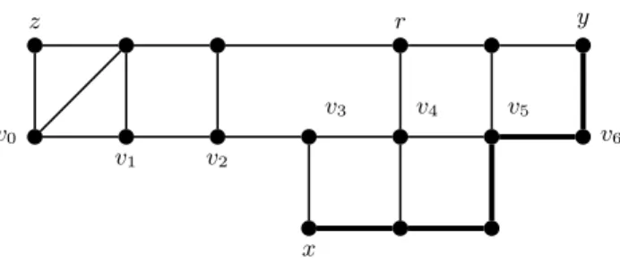
v0 v1 v2 v6 r z x y v3 v4 v5

Fig. 1.The bound shown in Theorem 2 is tight. Indeed the graph is such that v0, v1...v6

is a shortest path of eccentricity 1. The vertex z is at distance 5 from the shortest path (shown by thick edges) between x and y computed by double-BFS starting at r.

Theorem 2. A double-BFS is a linear-time 5-approximation algorithm for the MESP problem.

Before we prove it, notice that Figure 1 shows that this bound is tight.

Proof. Let k be k(G), P = v0, v1...vtbe a MESP (its eccentricity is thus k), and

Q= x, ..., y be the result of a double-BFS starting at some arbitrary vertex r, then reaching x, then reaching y. We shall prove that Q is a 5k-dominating path of G.

Let i (resp. j) be such that vi (resp. vj) is at distance at most k of r (resp.

x). The following inequalities are verified:

d(r, x) ≥ d(r, vt) ≥ d(vi, vt) − d(r, vi) ≥ d(vi, vt) − k (6)

d(r, x) ≤ d(r, vi) + d(vi, vj) + d(vj, x) ≤ d(vi, vj) + 2k (7)

Combining those inequalities,

d(vi, vt) − 3k ≤ d(vi, vj) (8)

Similarly:

d(vi, v0) − 3k ≤ d(vi, vj) (9)

Therefore vj is at distance at most 3k of v0or vt. Without loss of generality,

assume that vj is at distance at most 3k of v0.

Let l be such that vlis at distance at most k of y. We distinguish two cases:

(i) l ≤ j:

Then y is at distance at most 5k of x. As y is a vertex most distant from x, x is a 5k-dominating vertex of the graph. The lemma is then verified.

(ii) l > j :

Applying to (x, y) the inequalities established at the beginning of the proof:

d(vj, vt) − 3k ≤ d(vj, vl) (10)

As l > j, it follows that:

d(vl, vt) ≤ 3k (11)

Figure 2 shows the configuration of the graph in that case. The vertices at distance at most k of a vertex vs such that s ≤ j (resp. s ≥ l) are at

distance at most 5k of x (resp. y).

According to Lemma 1, every vertex v of G at distance at most k of a vertex vs such that s is between j and l is at distance at most 3k of any

shortest path between x and y. The lemma is thus verified.

v0 v1 vj vi vl vt−1 vt x r y ≤k ≤k ≤k max v∈G d(r, v) max v∈G d(x, v)

Fig. 2.Notations used in the proof of Theorem 2

3

A 3-Approximation Algorithm

We show now that by using more BFS runs we may obtain a 3k-approximation of MESP, still in linear time.

Let bestPath and bestEcc be global variables used as return values for the path and its eccentricity. bestPath stores a path and is uninitialized, and bestEcc is an integer initialized with |V (G)|.

Data: G graph, x,y vertices of G, step integer

1 Compute a shortest path Q between x and y; 2 Select a vertex z of G most distant from Q; 3 if d(Q, z) < bestEcc then 4 bestP ath← Q; 5 bestEcc← d(Q, z); 6 end 7 if step < 8 then 8 Algorithm3k(G,x,z,step + 1); 9 Algorithm3k(G,y,z,step + 1); 10 end Algorithm 1: Algorithm3k

Theorem 3. A 3-approximation of the MESP Problem can be computed in lin-ear time by considering a spread pair (s, l) of G and running Algorithm3k(G,s,l,0).

Proof (Correctness). Let G be a graph admitting a shortest path P = v0, v1...vt

of eccentricity k.

Let x and y be any vertices of G, Qx,y a shortest path between x and y.

Define ix,ymin (resp. ix,ymax) as the smallest (resp. largest) integer such that vix,y_min

(resp. vix,ymax) is at distance at most k of x or y. Then, by Lemma 1,

For all j such that ix,ymin− k ≤ j ≤ i x,y

max+ k, d(Qx,y, vj) ≤ 2k (12)

Hence, if ix,ymin≤ k and ix,ymax≥ t − k, every vertex of P is at distance at most

2k of Qx,y and, as P is of eccentricity k, Qx,y is of eccentricity at most 3k.

Algorithm3k uses this implication to exhibit a pair x, y such that Qx,y is of

eccentricity at most 3k. Indeed, in each recursive call, one of the following cases holds:

1. the vertex z selected at line 3 is at distance at most 3k from Qx,y. In that

case, bestPath will be set to Qx,y unless it already contains a path of even

better eccentricity. In any case, the result of the algorithm is a path of eccentricity at most 3k.

2. the vertex z is at a distance greater than 3k of Qx,y. Let iz be such that viz

is at distance at most k of z. Then, according to Equation (12),

iz≤ ix,ymin− k or iz≥ ix,ymax+ k (13)

(a) Suppose that iz ≥ ix,ymax+ k. Then, in the case d(vix,y_min, x) = k, we get

ix,z_min≤ ix,ymin and i x,z

max≥ ix,ymax+ k. And in the case d(vix,y_min, y) = k we get

ix,zmin≤ i x,y

min− k and ix,zmax≥ ix,ymax.

(b) A similar reasoning can be applied if iz ≤ ix,ymin− k, also yielding to

ix,zmin≤ i x,y

min and ix,zmax≥ ix,ymax+ k or i x,z min≤ i

x,y

Therefore, either the algorithm already found a path of eccentricity at most 3k, or it makes one of its two new calls with a couple (x′_{, y}′_{) such that the}

interval [ixmin′,y′, i x′_,y′ max] contains [i x,y min, i x,y

max] but has length increased by at least k.

Consider now a spread pair (s, l) for which Algorithm3k(G,s,l,0) is run. It follows from case (i) and (ii) of the proof of Theorem 2 that

is,lmin≤ 5k and i s,l

max≥ t − 5k (14)

At each of the recursive calls, if no path of eccentricity at most 3k has already been discovered, one of the new calls expands the interval [ix,ymin, ix,ymax] length by

at least k, while containing the previous interval. As the recursive calls are made until step = 8, it follows that either a path of eccentricity 3k has been discovered, or one of the explored possibilities corresponds to eight extensions of size at least kstarting from [is,lmin, i

s,l max].

In the latter case, Equation (14) implies that the final couple of vertices (x, y) fulfills ix,ymin≤ k and i

x,y

max≥ t − k. Every vertex of P is then of distance at most

2k of Qx,y and thus Qx,y is of eccentricity at most 3k.

Proof (Complexity). The algorithm computes two BFS trees at line 1 and 2, taking O(n + m) time. The rest of the operations is computed in constant time. The recursivity width is 2 and, since it is first called with step = 0, the recursivity length is 8. The algorithm is thus called 255 times. Therefore the total runtime of the algorithm is O(n + m).

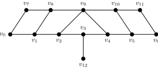
Proof (Tightness of the approximation). Figure 3 shows a graph for which the algorithm may produce a path of eccentricity 3k(G) (see caption).

v0 v1 v2 v3 v4 v5 v6 v7 v8 v9 v10 v11 v12

Fig. 3. Tightness of the bound shown in Theorem 3. The algo-rithm may indeed loop between the following couples of vertices : (v0, v6), (v0, v12), (v6, v12), (v0, v11), (v11, v12), (v6, v7), (v7, v12), (v11, v7). Each time, it

may choose a shortest path of eccentricity 3 (passing through v8 v9 and v10 whenever

4

Bounds between MESP and Laminarity

In this section, we investigate the link between the MESP problem and the notion of laminarity introduced by V¨olkel et al. in [12]. The study of the k-laminar graph class finds motivation both from a theoretical and practical point of view. On the theoretical side, AT-free graphs form a well known graph class introduced half a century ago by Lekkerkerker and Boland [10], which contains many graph classes like co-comparability graphs. An AT-free graph admits a diameter all other vertices are adjacent with [5]. It is then natural to extend this notion of dominating diameter. On the practical side, some large graphs constructed from reads similarity networks of genomic or metagenomic data appear to have a very long diameter and all vertices at short distance from it [12], and exhibiting the ”best” diameter allows to better understand their structure.

Definition 2 (laminarity). A graph G is

– l-laminar if G has a diameter of eccentricity at most l.

– s-strongly laminar if every diameter has eccentricity at most s.

l(G) and s(G) denote the minimal values of l and s such that G is respectively l-laminar and s-strongly laminar.

A natural question about laminarity and MESP is to ask what link exists between them.

Theorem 4. For every graph G,

k(G) ≤ l(G) ≤ 4k(G) − 2 k(G) ≤ s(G) ≤ 4k(G)

Moreover, there exist three graph sequences (Gk)k≥1, (Hk)k≥1 and (Jk)k≥1

such that, for every k,

– k(Gk) = l(Gk) = s(Gk) = k;

– k(Hk) = k and l(Hk) = 4k − 2;

– k(Jk) = k and s(Jk) = 4k;

The bounds given by the inequalities are therefore tight. Proof (k(G) ≤ l(G) and k(G) ≤ s(G)).

Those inequalities are straightforward as every diameter is by definition a shortest path. The eccentricity of every diameter is therefore always greater than k(G).

Proof (s(G) ≤ 4k(G)).

Let D = x0, x1, ...xs be a diameter of G and P = v0, v1...vt a shortest path

of eccentricity k. We shall show ecc(D) ≤ 4k. Let z be any vertex of G. Since ecc(P ) = k there exists a vertex viof P such that d(z, vi) ≤ k. Let us distinguish

three cases:

• Case 1: there exists vertices xa, xbof D and va, vbof P such that a ≤ i ≤ b

and d(va, xa) ≤ k and d(vb, xb) ≤ k. Then by Lemma 1, z is at distance at most

3k from any shortest path between xa and xb, and thus at distance at most 3k

of D.

• Case 2: there exists no vertex va of P with a ≤ i and d(va, D) ≤ k

• Case 3: there exists no vertex va of P with i ≤ a and d(va, D) ≤ k.

Without loss of generality we focus on Case 2 (illustrated in Figure 4), which is symmetric with Case 3. Let l (resp. m) be such that vl(resp. vm) is at distance

at most k of x0(resp. xs), assume l ≤ m:

d(vl, vm) ≥ d(x0, xs) − 2k (15)

Dbeing a diameter,

d(x0, xs) ≥ d(v0, vt) (16)

By combining those inequalities,

d(vl, vm) ≥ d(v0, vt) − 2k (17)

d(vl, vm) ≥ d(v0, vi) + d(vi, vl) + d(vl, vm) + d(vm, vt) − 2k (18)

2k ≥ d(vi, vl) (19)

It follows that z is at distance at most 4k of x0.

Proof (l(G) ≤ 4k(G) − 2).

Let D = x0, x1, ...xs be a diameter of G and P = v0, v1...vt a shortest path

of eccentricity k. We shall show that either ecc(D) ≤ 4k − 2 or G contains a diameter D′ _{of eccentricity 3k. If P is a diameter we are done. Let us suppose}

from now it is of length at most |D| − 1.

Let z be any vertex of G and vi a vertex of P such that d(z, vi) ≤ k. Let

us distinguish the same three cases than in the proof that s(G) ≤ 4k(G). The first case also leads to d(z, D) ≤ 3k. The second and third being symmetric, let us suppose there exists no vertex vj of P at distance at most k of D such that

j≤ i.

Let vl (resp. vm) be a vertex of P at distance at most k from x0 (resp. xs),

clearly,

d(vl, vm) ≥ |D| − 2k. (20)

Let us distinguish two subcases:

• Case 2.1: d(vl, vm) > |D| − 2k,

It follows that z is at distance at most 4k − 2 of D. • Case 2.2: d(vl, vm) = |D| − 2k

In this case, a path D′ _{= x}

0, ..vl, vl+1, ..vm, ..xs is a diameter. Assuming

l≤ m, Equation 19 in previous proof shows that:

d(vi, vl) ≤ 2k (22)

and with a symmetrical reasoning,

d(vm, vt) ≤ 2k (23)

It follows that any vertex v of G at distance at most k of a vertex va with

a≤ l (resp. a ≥ m) is at distance at most 3k of vl(resp. vm). Hence at distance

at most 3k of D′_{. v}

l, vl+1, ..vm being a subpath of D′, any vertex v of G at

distance at most k of a vertex va with a between m and t is at distance at most

k of D′_{. Finally, any vertex of G is at distance at most 3k of D}′_.

v0 vi vl vm vt z x0 xs ≤2k ≥diam(G) − 2k ≤k ≤k ≤k diam(G)

Fig. 4.Notations used in Case 2 of the proof of Theorem 4

Proof (Tightness of the bounds).

Consider the graph Gk reduced to a path P of length 4k to which a second

path of length k is attached in the middle. P is then simultaneously the only diameter and the MESP, and it k-covers Gk but doesn’t (k − 1)-cover it. Hence

the inequalities k(G) ≤ l(G) and k(G) ≤ s(G) are tight.

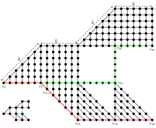
Figure 5 shows how to build the graph sequence (Jk)k≥1(only J1and J6are

drawn). Jk is a graph with a shortest path of eccentricity k and a diameter of

eccenticity 4k. The inequality s(G) ≤ 4k(G) is thus tight.

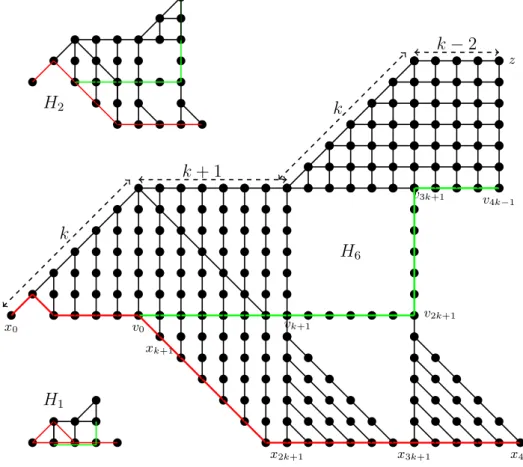
Figure 6 shows how to build the graph sequence (Hk)k≥1 (only H1, H2 and

and H6are drawn). Hkis a graph with a shortest path of eccentricity k, while the

unique diameter has eccenticity 4k − 2 (H1is a special case with two diameters).

x0 v0 v2k v4k z xk+1 x2k x3k x4k vk v3k

k

k

k

k

Fig. 5.Proof that s(G) ≥ 4k(G). The red path x0, x1, ...x4k is a diameter of length 4k

and at distance 4k of z; while the green path v0, v1, ...v4k is a shortest path (another

diameter indeed) of eccentricity k. The large graph is J6 (using the graph sequence

(Jk)kfrom Theorem 4) and the small one on the bottom left is J1. The other members

of the sequence car easily be derived. .

5

Conclusion

We have investigated the Minimum Eccentricity Shortest Path problem for gen-eral graphs and proposed a linear time algorithm computing a 3-approximation. The algorithm is a 2-recursive function with constant recursivity depth, launch-ing two BFSs each time, thus taklaunch-ing linear time. Additionally, we’ve established some tight bounds linking the MESP parameter k(G) and the k-laminarity pa-rameters s(G) and l(G).

On improving the current approximation algorithms, the following remark should be noted. Our algorithm is confined in finding a good pair of vertices in the graph, and the shortest path between them is then picked arbitrarily. By doing so, we are unlikely to get a better result than a 3-approximation. Indeed as shown by [9] there exist graphs for which the MESP solution is a path of

eccentricity k between two vertices s and t such that some other shortest paths between s and t have an eccentricity of exactly 3k.

About laminarity parameters, computing l(G) is NP-complete, while com-puting s(G) can be done in O(n2

mlog n) time [12]. It may be interesting to design an approximation algorithm, i.e producing a diameter of eccentricity at most αs(G) or βl(G). Linear-time algorithms like BFS cannot be used however, since we do not know how to compute diam(G) faster than a matrix product,

x0 v0 v2k+1 v4k−1 z xk+1 x2k+1 x3k+1 x4k vk+1 v3k+1

k

k + 1

k

k

_{− 2}

H

H

H

Fig. 6.Proof that l(G) ≥ 4k(G) − 2. It is a graph sequence (Hk)k, using the notation

from Theorem 4. For k ≥ 2, the red path x0, x1, ...x4kis the unique diameter. Its length

is 4k and it is at distance 4k − 2 of z. The green path v0, v1, ...v4k−1 is a shortest path

of length 4k − 1 and of eccentricity k. Graphs H2and H6are drawn but all graphs Hk,

k ≥2 can be derived from the pattern of H6. The small graph on the bottom left is

the special case H1 who do not follow this pattern. It admits exactly two diameters,

both of eccentricity 2 (red), and a shortest path of eccentricity 1 (green). .

and even surlinear approximation are studied [1]. Different techniques than the ones used here must therefore be employed.

References

1. Aingworth, D., Chekuri, C., Indyk, P., Motwani, R.: Fast estimation of diameter and shortest paths (without matrix multiplication). SIAM J. Comput. 28(4), 1167– 1181 (1999), http://dx.doi.org/10.1137/S0097539796303421

2. Bacs´o, G., Tuza, Z., Voigt, M.: Characterization of graphs dominated by induced paths. Discrete Mathematics 307(7-8), 822–826 (2007), http://dx.doi.org/10.1016/j.disc.2005.11.035

3. Corneil, D.G., Dragan, F.F., K¨ohler, E.: On the power of BFS to determine a graph’s diameter. Networks 42(4), 209–222 (2003), http://dx.doi.org/10.1002/net.10098

4. Corneil, D.G., Olariu, S., Stewart, L.: A linear time algorithm to compute a dominating path in an at-free graph. Inf. Process. Lett. 54(5), 253–257 (1995), http://dx.doi.org/10.1016/0020-0190(95)00021-4

5. Corneil, D.G., Olariu, S., Stewart, L.: Asteroidal triple-free graphs (1997), http://dx.doi.org/10.1137/S0895480193250125

6. Corneil, D.G., Olariu, S., Stewart, L.: Linear time algorithms for dominating pairs in asteroidal triple-free graphs. SIAM J. Comput. 28(4), 1284–1297 (1999), http://dx.doi.org/10.1137/S0097539795282377

7. Deogun, J.S., Kratsch, D.: Diametral path graphs. In: Nagl, M. (ed.) Graph-Theoretic Concepts in Computer Science, 21st International Workshop, WG ’95, Aachen, Germany, June 20-22, 1995, Proceedings. Lecture Notes in Computer Sci-ence, vol. 1017, pp. 344–357. Springer (1995), http://dx.doi.org/10.1007/3-540-60618-1 87

8. Deogun, J.S., Kratsch, D.: Dominating pair graphs. SIAM J. Discrete Math. 15(3), 353–366 (2002), http://dx.doi.org/10.1137/S0895480100367111

9. Dragan, F.F., Leitert, A.: On the minimum eccentricity shortest path problem. In: Dehne, F., Sack, J., Stege, U. (eds.) Algorithms and Data Structures - 14th International Symposium, WADS 2015, Victoria, BC, Canada, August 5-7, 2015. Proceedings. Lecture Notes in Computer Science, vol. 9214, pp. 276–288. Springer (2015), http://dx.doi.org/10.1007/978-3-319-21840-3 23

10. Lekkerkerker, C., Boland, J.: Representation of a finite graph by a set of intervals on the real line. Fund. Math. 51, 45–64 (1962)

11. Robertson, N., Seymour, P.D.: Graph minors. i. excluding a forest. J. Comb. The-ory, Ser. B 35(1), 39–61 (1983), http://dx.doi.org/10.1016/0095-8956(83)90079-5 12. V¨olkel, F., Bapteste, E., Habib, M., Lopez, P., Vigliotti, C.: Read networks and

k-laminar graphs. CoRR abs/1603.01179 (2016), http://arxiv.org/abs/1603.01179 13. Yamazaki, K., Bodlaender, H.L., de Fluiter, B., Thilikos, D.M.: Isomorphism for graphs of bounded distance width. In: Bongiovanni, G.C., Bovet, D.P., Battista, G.D. (eds.) Algorithms and Complexity, Third Italian Conference, CIAC ’97, Rome, Italy, March 12-14, 1997, Proceedings. Lecture Notes in Computer Science, vol. 1203, pp. 276–287. Springer (1997), http://dx.doi.org/10.1007/3-540-62592-5 79

14. Yan, S., Xu, D., Zhang, B., Zhang, H., Yang, Q., Lin, S.: Graph embedding and extensions: A general framework for dimensionality re-duction. IEEE Trans. Pattern Anal. Mach. Intell. 29(1), 40–51 (2007), http://dx.doi.org/10.1109/TPAMI.2007.250598