HAL Id: hal-01946539
https://hal.archives-ouvertes.fr/hal-01946539v5
Submitted on 15 Mar 2020
HAL is a multi-disciplinary open access
archive for the deposit and dissemination of
sci-entific research documents, whether they are
pub-lished or not. The documents may come from
teaching and research institutions in France or
abroad, or from public or private research centers.
L’archive ouverte pluridisciplinaire HAL, est
destinée au dépôt et à la diffusion de documents
scientifiques de niveau recherche, publiés ou non,
émanant des établissements d’enseignement et de
recherche français ou étrangers, des laboratoires
publics ou privés.
Computation of sum of squares polynomials from data
points
Bruno Després, Maxime Herda
To cite this version:
Bruno Després, Maxime Herda. Computation of sum of squares polynomials from data points. SIAM
Journal on Numerical Analysis, Society for Industrial and Applied Mathematics, 2020, 58 (3),
pp.1719-1743. �10.1137/19M1273955�. �hal-01946539v5�
BRUNO DESPR ´ES˚ AND MAXIME HERDA:
Abstract. We propose an iterative algorithm for the numerical computation of sums of squares of polynomials approximating given data at prescribed interpolation points. The method is based on the definition of a convex functional G arising from the dualization of a quadratic regression over the Cholesky factors of the sum of squares decomposition. In order to justify the construction, the domain of G, the boundary of the domain and the behavior at infinity are analyzed in details. When the data interpolate a positive univariate polynomial, we show that in the context of the Lukacs sum of squares representation, G is coercive and strictly convex which yields a unique critical point and a corresponding decomposition in sum of squares. For multivariate polynomials which admit a decomposition in sum of squares and up to a small perturbation of size ε, Gεis always coercive and so it minimum yields an approximate decomposition in sum of squares. Various unconstrained descent algorithms are proposed to minimize G. Numerical examples are provided, for univariate and bivariate polynomials.
Key words. Positive polynomials, sum of squares, convex analysis, positive interpolation, iterative methods. AMS subject classifications. 90C30, 65K05, 90C25
1. Introduction. The numerical and algorithmic motivation of the present paper comes from a recent work [5] where an iterative algorithm for positive interpolation (meaning that a sign condition on a given closed interval I must be respected) was proposed for of univariate polynomials. A prac-tical scenario which illustrates the interest of iterative positive interpolation is the following. Take a polynomial without knowing its sign on I. If the iterative method converges and recover p at the limit (it can be checked at a finite number of points), then p is non negative on I (that is for an infinite number of points). In this case the algorithm provides an iterative certificate of positivity [14,15]. But if the iterations do not recover p at the limit (or if one stops the algorithm after a finite number of iterations), then p is (or might be) non positive on I. In this case of non convergence, the iterations provide nevertheless a non negative surrogate to p. We refer to the quoted work for an illustration of the interest of non negative polynomial surrogates in the context of Scientific Computing (SC). However two important restrictions in the previous algorithm [5] are that the polynomials are univariate and the interpolation points, where the data of the polynomials are given, are sliding points (it allowed for strong convergence properties). It brings severe constraints for applications in SC. In the present work, we relax these restrictions by constructing a new iterative algorithm for positive interpolation. The algorithm aims at computing a sum of squares (SOS) decomposition from the sole knowledge of prescribed interpolation data at prescribed interpolation points. Also the method is much more general so it is formulated for multivariate polynomials as well and does not need tensorization, something that was impossible with the previous method.
A modern reference in SC for control of the sign of polynomials at a finite number of prescribed interpolation points is in the works of C.-W. Shu [27], with application to the discretization of hyperbolic equations with high order methods. The point of view developed in this article is to control the sign of polynomials on all points in a given compact (semi-algebraic) set K Ă Rd which is much more
demanding. Preliminary tests for the construction of such algorithms are in [6], but the methods were inefficient in terms of the time of restitution. In a fully different direction, one must mention the theory of numerical approximation with splines, see [16,2]: splines are widely used in scientific computing and computer aided design (CAD) but often needs tensorization in multi-dimension; this limitation is not encountered by our new methods because they can be implemented on any semi-algebraic set K in any
˚Sorbonne-Universit´e, CNRS, Universit´e de Paris, Laboratoire Jacques-Louis Lions (LJLL), F-75005 Paris, France, and Institut Universitaire de France
:Inria, Univ. Lille, CNRS, UMR 8524 Laboratoire Paul Painlev´e, F-59000 Lille, France 1
dimension.
In the community of numerical optimization [14] from which we borrow most of our notations, SOS algorithms based on SemiDefinite Programming (SDP) are extensively used. It had been noticed by Powers and W¨ormann [24] that finding an SOS decomposition is equivalent to SDP, that is optimization in the cone of non-negative quadratic forms. Then algorithms based on interior-point methods were developed to solve these problems [21, 20, 28]. However, these methods seem to be hardly directly applicable in SC because they are based more on algebraic properties and not on interpolation data which are of major importance in numerical analysis and SC. This leads us to the development of the algorithm of the present paper, which is not based on SDP but rather on the iterative resolution of a non-convex quadratic problem over Cholesky factors of the SOS decomposition. We solve the quadratic program using a dualization of the problem, which leads us to a nonlinear convex program. Let us mention that a similar reformulation of general SDP was proposed by Burer and Monteiro [4]. In our case however, we use the particular structure of the interpolation data of the SOS to obtain some useful coercivity properties on the dual function. Also, similar dualization ideas can be found in [18, 10], but unlike here they are formulated on the Gram matrix rather than on the Cholesky factors. Our construction will generate a functional with strong convexity properties for which standard descent algorithms are efficient, as shown in the numerical section.
Let PrXs :“ PrX1, . . . Xds be the set of real polynomials with d variables. The subset of polynomials
of total degree less than or equal to n ě 1 is denoted by Pn
rXs, with r˚“ dim PnrXs. Let K Ă R be a
closed semi-algebraic set defined through a finite number j˚ of polynomial inequalities
(1.1) K “ x P Rd such that gjpxq ě 0 for gjP PrXs, 1 ď j ď j˚( .
Most standard cells (intervals in 1D, squares and triangles in 2D, . . . ) in SC can be implemented as semi-algebraic sets, so it is not a restriction for further applications. The convex set of non-negative polynomials of maximal degree n on K is
(1.2) PnK,`rXs “ tp P PnrXs such that ppxq ě 0 for any x P Ku .
Famous examples of characterizations as SOS are the Lukacs theorem [29] or Putinar’s Positvstellensatz [25]: a recent state of the art can be found in the books of Lasserre [14, 15]; some recent algorithmic issues in the context of optimal control can be found in [12] and therein. In order to be constructive, we focus in this work on the following version
(1.3) p “ j˚ ÿ j“1 gj ˜i ˚ ÿ i“1 q2 ij ¸ “ i˚ ÿ i“1 ˜j ˚ ÿ j“1 gjq2ij ¸ “ j˚ ÿ j“1 i˚ ÿ i“1 gjqij2,
where the maximal number of squares is equal to a predefined value i˚ ě 1 independent of j. In this
work, the number of squares i˚ and the degree of the polynomials qij are prescribed in function of n,
see below (1.4) for the prescription on i˚ and (1.5) for the prescription the degree of the polynomials
qij. It can be compared with the Schm¨ugden’s or Putinar’s Positvstellensatz where the degree of the
polynomials qij can be exponentially large [22,14]. With our notations, it is sufficient to embed p in a
set of polynomials of larger degree, that is to say to take n " degppq, to recover this case.
Next, the notion of unisolvence which comes from the Finite Element Method (FEM) is convenient to formalize properties of interpolation points. A unisolvent set of points pxrq1ďrďr˚ is such that any
polynomial p P Pn
rXs is uniquely determined by its values yr“ ppxrq for 1 ď r ď r˚. The number i˚of
polynomials in the SOS (1.3) is a priori independent from the number of interpolation points. However in our context the function G below is more naturally constructed assuming that
That is why we will assume (1.4) throughout this work, except at early stages of the construction. With these notations, one formulates the notion of positive interpolation: it is a recent adaptation [5] to SC of the notion of a certificate of positivity for which the reader can find information in [14,15]. A practical way to understand the model problem below is the following: from the knowledge of the values of p at only a finite number of given interpolation points, get a control of the sign of p at infinite number of points (the whole set K).
Problem 1.1 (Iterative positive interpolation on K). Let p P PnK,`rXs. Take a unisolvent set pxrq1ďrďr˚, and consider the interpolated values yr“ ppxrq. From pxr, yrq1ďrďr˚, compute iteratively
polynomials pqijqij such that the SOS representation (1.3) holds at the limit.
The methods and results studied in this work can be summarized as follows. Consider the param-etrization
(1.5) qij P PnjrXs with nj“ tpn ´ degpgjqq{2u
where t¨u denotes the integer part of a real number. Consider the canonical basis made of monomials (but other basis can be taken as well, see Remark 2.1), with the standard multi-index notation α “ pα1, . . . , αdq P Nd, |α| “ α1` ¨ ¨ ¨ ` αd and Xα “ X1α1. . . X
αd
d . The polynomials qij write qijpXq “
ř
|α|ďnjc
ij
αXα and we store the coefficients in a vector of coefficients cij “ pcijαqα P Rrj where rj “
dimpPnjrXsq “ `d`nj
d ˘. Gather the coefficients c
i1, ci2, ..., cij˚ in a single column vector (called a
Cholesky factor) Ui “ `ci1, ci2, . . . , cij˚
˘t
P Rr˚ where r
˚ “
řj˚
j“1rj. Define the Hankel matrices
Dnj
α,βpXq “ X
αXβfor |α|, |β| ď n
j. Define the polynomial valued block matrix BpXq “ BpXqtP Rr˚ˆr˚
(1.6) BpXq “ diag`g1pXqDn1pXq, , . . . , gj˚pXqD
nj˚pXq˘ .
This matrix is a block diagonal localizing matrix [14]. The first diagonal block is square r1ˆ r1, . . . until
the last block which is square rj˚ˆ rj˚: all other terms are zero. By construction, one has the identity
(1.7) j˚ ÿ j“1 gjpXq i˚ ÿ i“1 qij2pXq “ i˚ ÿ i“1 ˜j˚ ÿ j“1 gjpXqqij2pXq ¸ “ i˚ ÿ i“1 xBpXqUi, Uiy .
Denote the evaluation of BpXq at interpolation points as Br “ Bpxrq P Rr˚ˆr˚. Define the function
G : Rr˚ Ñ R “ R Y t`8u with domain D “ tλ P Rr˚ such that I `řr˚
r“1λrBrą0u as follows. For
λ P D then (1.8) Gpλq “ tr » – ˜ I ` r˚ ÿ r“1 λrBr ¸´1fi fl` r˚ ÿ r“1 yrλr,
otherwise Gpλq “ `8. In the previous formula, trp¨q denotes the trace. Our main results are the following.
Theorem 1.2. The function G has the following properties:
1. It is a proper closed convex function. It is C8 on its non-empty open convex domain D, tends
to infinity at BD and is infinite everywhere else by definition.
2. Each λ P D defines computable polynomials pqijrλsq1ďiďr˚,1ďjďj˚ such that
(1.9) BG Bλr pλq “ yr´ j˚ ÿ j“1 gjpxrq r˚ ÿ i“1 q2 ijrλspxrq, 1 ď r ď r˚.
If λ˚ P D is a critical point of G, that is ∇Gpλ˚q “ 0, then the family pqijrλ˚sqij is solution to
Theorem 1.3 (Existence of critical points in D). It is proved in two cases. 1. Take d ą 1, K a semi-algebraic set and p P Pn
K,`rXs. Assume that a technical condition on
the linear independence of the matrices Br is satisfied. Then, up to an infinitesimally small
perturbation (the perturbed polynomialpε
has the interpolation data pyrεq1ďrďr˚), the function
Gε is strictly convex, coercive and admits a unique critical point in D.
2. Taked “ 1, K a segment and p ą 0 on K. Then the technical condition the linear independence of the matrices Br is satisfied. Moreover G is strictly convex, coercive and admits a unique
critical point in D.
Corollary 1.4 (Solution to Problem1.1). Under the hypothesis of Theorem 1.3, the minimum of G (or Gε) in D yields a SOS decomposition of p (or pε). It can be computed by standard descent
algorithms.
As stated in the introduction, a practical scenario which in our mind has interest for SC is the following. Take a polynomial without knowing its sign on K. If the descent method converges and recover p at the limit, then p is non negative on K. If the descent does not recover p at the limit, then for monovariate polynomials, p is non positive on K. It shows that the descent method provides an iterative certificate of positivity. In case of non convergence, the iterations provide nevertheless a non negative surrogate to p. We refer to [5] for an illustration of the interest of non negative polynomial surrogates.
The outline of this paper is as follows. In Section2, we propose a dual interpretation of Problem
1.1. This leads us to the introduction of the function G and its domain. Then, in Section3, we discuss necessary and sufficient conditions characterizing asymptotic properties and strict convexity of G. In Section 4, we show that for univariate positive polynomials on a segment, the former conditions are satisfied yielding strict convexity and coercivity of the associated function G. Besides, we provide a more precise description the structure of the domain. In Section5, we present the specific descent and Newton type methods we use to compute the critical points of G. In Section 6 we provide numerical illustrations of the efficiency of our new approach for computing SOS decomposition of polynomials in one variable on segment and two variables on triangle. Finally, we provide in Appendix A some additional theoretical results concerning the links between the asymptotic cone of the set D and the Lagrange polynomials in the case of univariate polynomials.
Acknowledgements. Both authors are greatly indebted to Jean-Bernard Lasserre and Didier Henrion for their kind explanations on the theory and state of the art of semidefinite programming and sum of squares and would like to thank them for their invitation at LAAS and for their hospitality. The authors would also like to thank the anonymous referees for their suggestions and comments which helped to improve the quality of this paper.
2. Construction of G (Proof of Theorem 1.2). The construction of G, leading to (1.8), is done by recasting the model problem1.1as the convex dual of a Quadratically Constrained Quadratic Program (QCQP) (see[3]). In order to have a more general discussion, we relax the condition (1.4) in this part and in the next Section2.1. It means that
i˚‰ r˚
is possible as well. The condition (1.4) is reintroduced end of Section2.1. We begin with some remarks on the objects introduced in the first section.
Remark 2.1. In the numerical experiments of Section6, we use other polynomials than the mono-mials in order to optimize the robustness and accuracy of the algorithms. It only changes the definition of the matrix BpXq in (1.6) and thus of Br “ Bpxrq but every result of this paper still hold. More
values by constraints of the type yr“ Lrppq where the family tLr: PnrXs Ñ R, r “ 1, . . . , r˚u is any
basis of the dual space of PnrXs. In the context of SC more precisely for the numerical resolution of
partial differential equations, one deals with data points in finite difference discretizations. However, if one is considering a finite volume discretization, one would rather work with mean values on some mesh cells. This variant is easily manageable with our method by choosing the adequate linear forms Lr and modifying the matrices Br accordingly.
Remark 2.2. An interesting consequence of the Caratheodory Theorem ([11, Theorem III.1.3.6 page 98]) is that if a formula like (1.3) holds for i˚ ą r˚, then a similar one holds also for i˚ “ r˚ (but for
different polynomials qij). Indeed the set W “
řj˚
j“1gjpXqPnjrXs2 is a closed convex cone embedded
in p P Pn
rXs. Therefore any convex combination of i˚ą r˚elements of W can be expressed as a convex
combination of only r˚ “ dim PnrXs elements of W (the coefficients of the convex combination can be
set to 1 after proper rescaling of the new qij).
2.1. Lagrangian duality (Theorem 1.2 item 1). In any dimension, the notation x¨, ¨y will denote the Euclidean dot product and } ¨ } will denote the associated norm. We define the algebraic manifold (2.1) U “ tU “ pU1, . . . , Ui˚q P pR r˚qi˚ such that i˚ ÿ i“1 xBrUi, Uiy “ yr for all 1 ď r ď r˚u.
The vectors Ui are called the Cholesky factors [20, 28] of the decomposition. With the unisolvence
assumption, finding a SOS (1.3) amounts to finding one element U P U. In order to find a U P U in a constructive manner, our strategy is to start at a given V (probably outside U) and to project on U in the quadratic norm. It writes as follows.
Problem 2.3. Take V “ pV1, . . . , Vi˚q P pR r˚qi˚ . Calculate U “ argmin UPU 1 2 ři˚ i“1}Ui´ Vi}2.
The vectors V “ pViqi may be thought of as a good initial guesses for the U “ pUiqi. The optimal
value of the cost does not matter. However Problem 2.3seems even harder to solve than the original problem we were concerned with. The finding is that the Lagrangian dual problem is endowed with good properties provided V is conveniently chosen. In this case, the new Problem 2.3 provides a way to determine an admissible U P U.
Still for any V, introduce the Lagrangian which is the sum of the functional and of the dualization of the constraint (2.1) with a Lagrange multiplier λ P Rr˚
LpU, λq “ 1 2 i˚ ÿ i“1 ˜ }Ui´ Vi}2` r˚ ÿ r“1 λrxBrUi, Uiy ¸ ´1 2xλ, yy where y “ pyrq1ďrďr˚.
The first-order optimality constraints are ∇UL “ 0 and ∇λL “ 0. The first-order optimality constraint
∇UL “ 0 is linear with respect to U. Define the symmetric matrix M pλq “ M pλqtP Rr˚ˆr˚
(2.2) M pλq “ I `
r˚
ÿ
r“1
λrBr
where I is the identity matrix in Rr˚ˆr˚. The condition ∇
UL “ 0 writes
(2.3) M pλqUi“ Vi for 1 ď i ď i˚ðñ M pλqU “ V.
If the multiplier λ P Rr˚ is such that the matrix M pλq is invertible, then the candidate solution U can
It is therefore natural to concentrate on a condition on λ such that M pλq is invertible. In order to obtain convexity properties in the following we even restrict λ to the set of positive definiteness of M pλq. To our knowledge, this at this stage that our analysis differs from the standard exposition of dual QCQP [3,11] and from other dualizations in the context of SOS [4,18,10].
Definition 2.4. The domain of positive definiteness of M is D “ tλ P Rr˚ | M pλqą0u Ă Rr˚. It
is an open set and it is non empty since0 P D.
For a Lagrange multiplier λ P D, the inverse transformation of (2.3) is Upλq “ M pλq´1V.
Then, one can evaluate the Lagrangian at Upλq. An elementary computation yields LpUpλq, λq “
1 2 ři˚ i“1 ` }Vi}2´@Vi, M pλq´1Vi D˘
´12xλ, yy. This motivates the introduction of the dual objective function GV: D ÝÑ R defined by (2.4) GVpλq “ i˚ ÿ i“1 @Vi, M pλq´1Vi D ` xλ, yy , and which one should think of as a function to be minimized.
Lemma 2.5. The function GV is smooth on D. The first and second derivatives are
(2.5) BGV Bλr pλq “ yr´ i˚ ÿ i“1 hUipλq, BrUipλqi and B2GV BλrBλs pλq “ 2 i˚ ÿ i“1 BrUipλq, M pλq´1BsUipλq . In particularGV is convex on D.
Proof. The proof stems from the identity BλrM pλq
´1 “ ´M pλq´1B
rM pλq´1 and the symmetry
of the various matrices involved. Convexity follows from the positivity of M pλq and the expression of second derivatives yielding@∇2G
Vpλqµ, µ D “ 2řii“1˚ @Aipµ, λq, M pλq´1Aipµ, λq D ě 0 where Aipµ, λq “ řr˚ r“1µrBrUipλq for 1 ď i ď i˚.
In order to address the behavior of GV near the boundary, we will make us of the following notion.
Definition 2.6. A convex function f : Rr˚
ÞÑ R Y t`8u is said to be closed over its domain Df “ tx | f pxq ă 8u if and only if the level sets tx | f pxq ď tu are closed for t ă `8: see [11] or [3,
Appendix A.3.3.].
This property is extremely important in our approach because it yields a strong control of the objective function at finite distance.
Lemma 2.7. Assume the equality of dimensions (1.4))1, that is i˚ “ r˚, and that V P Rr˚ˆr˚ is
an orthogonal matrix. Then one has the simpler expression where trp¨q denotes the trace of a square matrix
(2.6) Gpλq :“ GVpλq “ trpM´1pλqq ` xλ, yy .
Moreover the extension of G :“ GV with value `8 outside of D is a closed convex function with open
domain D.
Proof. The formula is a direct consequence of (2.4), because the number i˚ of orthogonal vectors
Vi is equal to the dimension r˚ of the space. Thanks to the continuity on D, the closedness of GV on
Rr˚ amounts to showing that for any sequence pµ
kqk in D converging to a point of the boundary of
the domain BD “ λ P D | det pI ` řr˚
r“1λrBrq “ 0( , then one has GVpµkq Ñ `8 as k Ñ `8. In the
light of the representation formula (2.6) involving the trace of M pλq´1 it is the case since the minimal
eigenvalue of M pµkq goes to 0 as k Ñ `8. Clearly the function is independent of V.
1As a consequence, the notation i
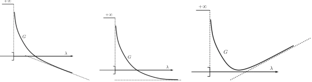
In order to have a better intuition of the structure of G, an illustration of its graph is given on Figure 1. Near the boundary of its domain, the function G behaves by construction like a rational barrier function [21, 3]. This barrier does not introduce any kind of approximation, and it is an exact one. This property is a strong algorithmic asset of G with respect to more standard logarithmic barrier methods. The figure provides three different illustrations of a closed convex function which is infinite outside of its domain. Actually we will show in the sections below that G is linear at infinity (in the direction of the asymptotic cone). The whole point will be to understand under which conditions G is coercive, which corresponds to the rightmost plot on Figure1. It will prove the existence of a multiplier in D, without explicitly requiring to use the methods of Lagrangian duality.
G `8 λ G `8 λ G `8 λ
Fig. 1. Three cases of the graph of a closed convex function f which is convex over its open domain and asymptotically linear at infinity. On the left, the function is not lower bounded and not coercive. In the center the function is lower bounded but not coercive. On the right, the function is lower bounded and coercive.
Even if the Lagrange multiplier λ is constrained in the domain D, the minimization of the dual func-tion G can be done by essentially unconstrained descent algorithms thanks to its coercivity properties. We will make this clearer in Section5. This behavior is another asset of the function G.
2.2. Critical points of G (Theorem 1.2 item 2). In this section, we formalize natural con-sequences of the formulas (2.5) for the derivatives of G, which are preparatory to establish that the G is naturally coercive in the domain D. These first properties are essentially a reformulation of the previous material.
These first properties are essentially a reformulation of the previous material. For each Lagrange multiplier λ P D one defines the vectors pcij
αrλsqα,j P Rrj which are the components of Uipλq, the
latter being the ith column of M pλq´1. It defines the polynomials q
ijrλs P PnjrXs by qijrλspXq “
ř
|α|ďnjc
ij
αrλsXα. With (1.7), these polynomials define a sum of square prλs P PnK,`rXs
(2.7) prλspXq “ j˚ ÿ j“1 gjpXq ˜r˚ ÿ i“1 qij2rλspXq ¸ . Using (1.7), prλspxrq “ řr˚ i“1hBrUi, Uii. So (2.5) is rewritten as (2.8) BG Bλr pλq “ yr´ prλspxrq.
The Proposition below characterizes that in order to solve Problem1.1it is sufficient to find critical points of G. It is part of the Lagrangian duality between the primal formulation of Problem2.3and the dual formulations (2.4) or (2.6).
Proposition 2.8. Take p P PnK,`rXs and an unisolvent set of interpolation points pxrq1ďrďr˚ in
‚ λ˚ P D is a critical point of G, namely ∇Gpλ˚q “ 0. ‚ λ˚ P D minimizes G.
‚ ppXq “ prλ˚spXq.
Proof. Since G is closed convex, local minima coincide exactly with critical points, so the first two points are equivalent. The equivalence between the first and third assertions follows from (2.8) and the unisolvence assumption.
2.3. Number of squares. Let us precise the number of squares in the SOS formula (2.7). This information is additional with respect to Theorem 1.2. It brings the possibility to have a cheaper implementation.
Lemma 2.9. The number of non zero polynomials inřri“1˚ q 2
ijrλspXq is less or equal to rj.
Proof. By construction`U1pλq, . . . , Ur˚pλq
˘
“ Upλq “ M pλq´1 is a block diagonal matrix. The blocks have size r1ˆ r1 until rj˚ˆ rj˚. So, for a given j, the polynomials qijrXs vanish for 1 ď i ď
r1` ¨ ¨ ¨ ` rj´1and for r1` ¨ ¨ ¨ ` rj´1` rj` 1 ď i ď r˚.
Remark 2.10. The result of Lemma 2.9 is nevertheless non optimal in dimension d “ 1. Indeed consider the Luk´acs Theorem (see Proposition4.1) in the odd case n “ 2k ` 1 and take g1pXq “ X and
g2pXq “ p1 ´ Xq as in (4.3). So r˚ “ n ` 1 and r1“ r2“ k ` 1. Assume that there exists a critical point
λ˚ to G. Then (2.7) yields a representation ppXq “ X
řk
i“1p2i1rλ˚spXq ` p1 ´ Xq
ř2k
i“k`1p2i2rλ˚spXq.
In terms of the number of squares, here 2k, it is clearly non optimal with respect to the result of the Luk´acs Theorem which involves only two polynomials whatever n.
3. Coercivity of G (Proof of Theorem 1.3 Item 1). A sufficient condition for the existence of a critical point is that G is infinite at infinity, this is called coercivity,
(3.1) lim
}λ}Ñ`8
Gpλq “ `8.
A sufficient condition for the uniqueness of the critical points is strict convexity.
In the following, we start in Section3.1 by investigating the asymptotic behavior of G along rays starting at 0. From this knowledge we derive conditions characterizing coercivity in Section 3.2. We characterize strict convexity in Section3.3.
3.1. The asymptotic cone. There are two types of directions in D. For d P Rr˚ with }d} “ 1,
one defines the rays Rd :“ tλ “ td | t ě 0u issued from the starting point 0 P Rd. Two possibilities
occur: either Rdintersects the boundary BD either it does not. In the first case if one notes tdą 0 the
unique real number such that tdd P BD, then limtÑt´
d Gptdq “ `8. So the function G is bounded from
below and coercive in the direction d.
In this section one is interested in the rest of the directions. They generate the so-called asymptotic cone or recession cone of D. The asymptotic cone is closed, independent of the starting point and is classically defined [11] by C8 “ tλ P Rr˚ such that @µ P D, t ě 0, µ ` tλ P Du.
Lemma 3.1. The asymptotic cone of D is C8“ tλ P Rr˚ |
řr˚
r“1λrBrľ0u.
Proof. Let λ, µ such thatřr˚
r“1λrBrľ 0 and I `
řr˚
r“1µrBrą 0. Then, I `
řr˚
r“1pµr` tλrqBrą 0
for all t ě 0, so λ belongs to the asymptotic cone. Conversely let λ such that for all µ and t ě 0, µ ` tλ P D. Ifřr˚
r“1λrBrhad a negative eigenvalue then for t large enough I ` tř r˚
r“1λrBr would also
have a negative eigenvalue which would contradict the fact that tλ P D. The main question is the asymptotic behavior of G in directions in C8.
Some preparatory material is provided. One introduces the polynomial valued vector LpXq with components being the Lagrange polynomials associated with the set of points pxrq1ďrďr˚ evaluated at
x, namely
(3.2) LpXq “ plrpXqq1ďrďr˚ P Rr˚,
where the Lagrange interpolation polynomials lrP PnrXs are defined by lrpxsq “ δrsfor 1 ď r, s ď r˚,
where δrs denotes the Kronecker symbol. The vector LpXq will be called a Lagrange vector. The
polynomial p which takes the value yrat xr satisfies the Lagrange interpolation formula
(3.3) ppXq “
r˚
ÿ
r“1
yrlrpXq “ xy, LpXqy .
One can show another interpolation property characteristics of our problem.
Lemma 3.2. One has BpXq “řrr“1˚ lrpXqBr. For x P K, Bpxq is positive semidefinite and Lpxq P
C8.
Proof. Let W, Z P Rr˚ be the coefficients of some polynomials pp
jq1ďjďj˚ and pqjq1ďjďj˚. By
definition (1.6-1.7) of Bpxq which is symmetric one knows that C W, ˜ Bpxq ´ r˚ ÿ r“1 lrpxqBr ¸ Z G “ j˚ ÿ j“1 ˜ gjpxqpjpxqqjpxq ´ r˚ ÿ r“1 lrpxqgjpxrqpjpxrqqjpxrq ¸ “ 0.
Since W, Z are arbitrary, it yields the first part of the claim. Also for x P K, one has that gjpxq ě 0.
Therefore xW1, BpxqW1y “ ř j˚
j“1gjpxqpjpxq2 ě 0 which yields that Bpxqľ0. One gets that Lpxq P
C8.
In the following there are three different results concerning the behavior of G in the asymptotic cone: either, Lemma 3.3, inftą0,λPC8Gptλq “ ´8; or, Proposition 3.4, inftą0,λPC8Gptλq ą ´8; or
even better, Proposition3.9, the function G is coercive.
Lemma 3.3. Assume that there exists z P K such that ppzq ă 0. Then limtÑ`8GptLpzqq “ ´8
and thus the corresponding functionG is not bounded from below in C8.
Proof. The half line generated by Lpzq is included in D by Lemma3.2and so all for t ě 0, one has G ptLpzqq “ tr`MptLpzqq´1˘
` tppzq. Since λ “ tLpzq P C8, one has M pλqľI so Gptλq ď r˚` tppzq ÝÑ tÑ8
´8.
Proposition 3.4. Consider p P PnK,`rXs, a unisolvent set of interpolation points pxrq1ďrďr˚ in K
and define yr“ ppxrq for 1 ď r ď r˚. The following properties are equivalent.
‚ For any λ P C8, one has xλ, yy ě 0.
‚ There exists polynomials qij for1 ď j ď j˚ and1 ď i ď r˚“ r˚ such that
ppXq “ j˚ ÿ j“1 gjpXq r˚ ÿ i“1 q2 ijpXq.
Proof. For W P Rr˚, define the vector s
W “ pxBrW, Wyq1ďrďr˚ P Rr˚. A equivalent definition
of C8 is C8 “ tλ P Rr˚ such that xsW, λy ě 0 for all W P Rr˚u. In order to prove the result, one
can invoke the Generalized Farkas Theorem ([11, Theorem III.4.3.4 page 131] with the correspondence y “ b). It already states that our first assertion is equivalent to y being in the closed convex conical hull of the linear forms sW, that is y “řri“1˚ αisWi where αiě 0 for all i, and r˚ is sufficiently large. It is
rewritten as y “řr˚
i“1sZi for Zi“ pαiq 1
3.2. Coercivity. Now we investigate the conditions such that G is infinite at infinity (coercivity). A first negative result about coercivity is the following. The proof easily adapted from the one of Lemma3.3.
Lemma 3.5. Assume there exists z P K such that ppzq “ 0. Then GptLpzqq remains bounded as t Ñ `8 and G is not coercive.
Thus we can only hope for coercivity starting from strictly positive polynomials. Let us know define a specific useful polynomial denoted as pB.
Definition 3.6. Define the polynomial pBpXq “ tr pBpXqq P PnK,`rXs, where BpXq is the matrix
defined in (1.6).
A key property of this polynomial is the following.
Lemma 3.7. Assume that the matrices tBru1ďrďr˚ are linearly independent. Then there exists a
constantc˚ą 0 such that
(3.4) c˚}λ} ď
r˚
ÿ
r“1
λrpBpxrq, @λ P C8.
Proof. Let λ P C8. The matrix
ř
rλrBris symmetric and positive semidefinite. So its matrix norm
can be controlled by its largest eigenvalue and thus by its trace, namely }řr˚
r“1λrBr} ď tr př r˚
r“1λrBrq “
řr˚
r“1λrpBpxrq. Second we also know that λ Ñř r˚
r“1λrBris injective thanks to the linear independence
assumption. Thus there a constant c˚ą 0 such that c˚}λ} ď }
řr˚
r“1λrBr}. Combining both inequalities
ends the proof.
Remark 3.8. The assumption of linear independence of tBru1ďrďr˚ is close but different than the
condition of Linear Independence Constraint Qualification (LICQ), see [23, Section 12.2], which in our setting says that the matrices tBrUu1ďrďr˚ are linearly independent for any matrix U such that
řr˚
i“1hBrUi, Uii “ yr for 1 ď r ď r˚. One may prove by contradiction that LICQ implies our
assumption.
Proposition 3.9. Let p P PnK,`rXs which admits a SOS (1.3). Take a unisolvent set of
in-terpolation points pxrq1ďrďr˚ in K and assume that the corresponding matrices tBru1ďrďr˚ are
lin-early independent. Take ε ą 0 and set pε
“ p ` εpB. Then the function Gε built from xr and
yε
r“ pεpxrq “ yr` εpBpxrq for 1 ď r ď r˚ is coercive.
Proof. The asymptotic cone C8 does not depend on y or yε and we desire to show firstly that
Gε grows linearly to infinity for directions in C
8. One has the identity
řr˚
r“1λryrε “
řr˚
r“1λryr`
εřr˚
r“1λrpBpxrq. Take λ P C8: proposition3.4yields
řr˚
r“1λryrě 0 because p is a SOS by assumption;
then Lemma3.7shows that for any λ P C8
řr˚
r“1λryrě 0 ` εc˚}λ} which yields uniform coercivity in
the directions in the asymptotic cone.
In order to show coercivity (3.1) which is a stronger statement, the proof is by contradiction. Assume it does not hold. Then there exists a constant K P R as well as a sequence ptm, dmqmPN
such that tm Ñ `8, }dm} “ 1 and Gptmdmq ď K. By convexity, and since Gp0q “ r˚, one has
Gptdmq ď maxpr˚, Kq for t P r0, tms. Up to the extraction of a sub-sequence there exists d˚ with
}d˚} “ 1, such that Gptd˚q ď maxpr˚, Kq for t P R`. In particular the ray with direction d˚ cannot
intersect the boundary BD so it belongs to the asymptotic cone C8. By the first estimate Gptd˚q ě εc˚t,
so it cannot be bounded which yields the contradiction.
3.3. Strict convexity. Strict convexity, if it holds, yields uniqueness of a critical point. This information is additional to Item 1 of Theorem1.3.
Proposition 3.10. Let p P PnK,`rXs be strictly positive on K. Take a unisolvent set of interpolation
points pxrq1ďrďr˚in K and assume that the corresponding matrices tBru1ďrďr˚are linearly independent.
ThenG is strictly convex over its domain D. Proof. From (2.5) one has that @∇2Gpλqµ, µD
“ 2řri“1˚ @Aipµ, λq, M pλq´1Aipµ, λq
D
ě 0 for all µ P Rr˚, where A
ipµ, λq “ přrr“1˚ µrBrqUipλq for 1 ď i ď r˚. Since M pλq´1 is positive definite, its
columns Uipλq form a basis.
By contradiction, assume now G is not strictly convex. There exists µ ‰ 0 such that@∇2Gpλqµ, µD “ 0. So the vectors Aipµ, λq vanish for all i. Soř
r˚
r“1µrBr“ 0, and µ “ 0 by linear independence of the
matrices pBrqr“1,...,r˚. This is a contradiction so ∇
2Gpλq ą 0 and G is strictly convex.
The strict convexity of G can be measured with the minimal eigenvalue of its Hessian αpλq “ infµ‰0 x
∇2G Vpλqµ,µy
}µ}2 ą 0, for any λ P D. An important property which motivates the design of one of
our numerical methods is the following.
Lemma 3.11. Under the assumptions of Proposition3.10, thenα has a cubic degeneracy at infinity in the interior of the asymptotic cone of D. For all d P Rr˚ such that }d} “ 1 andřr˚
r“1drBrą0, there
isCdą 0 such that αptdq ď Cdp1 ` tq´3 for all t ě 0.
Proof. Let λ “ td. For a constant C depending only on the data, one has @∇2Gpλqµ, µD ď C}M pλq´1}3
}µ}2. Under the assumptions the minimal eigenvalue of M pλq is given by 1 ` edt with ed
the minimal eigenvalue ofřr˚
r“1drBr. Hence }M pλq´1} “ Opp1 ` tq´1q.
4. Univariate polynomials on a segment (Theorem 1.3 Item 2). In this section, we focus on univariate polynomials, namely when d “ 1, over the segment K “ r0, 1s. This case is interesting because it is central for for numerical computation of functions of one variable and also one can easily prove the coercivity and the strict convexity. The notation is simplified by using the real variable x P R, more adapted to analytical methods.
We check that the various assumptions granting coercivity and strict convexity are satisfied. In view of Proposition3.4, Proposition3.9and Proposition3.10of the previous section, it suffices to exhibit an appropriate choice of functions pgjqjand of interpolation points such that: any non-negative polynomial
admits a (possibly non-explicit) SOS decomposition; and the matrices tBrur are linearly independent.
The first point follows from the Markov-Luk´acs Theorem, see [29,6,7,13] for a proof. Proposition 4.1 (Markov-Luk´acs). Let us consider p P Pnrxs and K “ r0, 1s.
‚ Even case: If n “ 2k, then p is non-negative on K if and only if there are polynomials a and b with degree less or equal to k and k ´ 1 respectively such that
(4.1) ppxq “ a2
pxq ` xp1 ´ xqb2pxq.
‚ Odd case: If n “ 2k ` 1, then p is non-negative on K if and only if there are polynomials a andb with degree less or equal to k such that
(4.2) ppxq “ xa2
pxq ` p1 ´ xqb2pxq. Now let us precise the setting. One takes j˚“ 2 and
(4.3)
#
for n is even : g1pxq “ 1 and g2pxq “ xp1 ´ xq,
for n is odd : g1pxq “ x and g2pxq “ 1 ´ x.
Concerning the interpolation points, we choose any r˚ “ n ` 1 distinct points pxrqr“1,...,n`1 on the
block structure (4.4) Br“ ˆ g1pxrqwr1b wr1 0 0 g2pxrqwr2b w2r ˙ P Rpn`1qˆpn`1q where $ & % for n “ 2k : wr1“`1, xr, . . . , xkr ˘t and wr 2“`1, xr, . . . , xk´1r ˘t , for n “ 2k ` 1 : wr 1“ wr2“`1, xr, . . . , xkr ˘t .
With these notations, the equalities (4.1) and (4.2) are equivalent to yr“ hBrU, Ui for 1 ď r ď n ` 1.
In the odd case n “ 2k ` 1 one has U “ pa0, . . . , ak, b0, . . . bkqt P Rn`1 with apxq “ řkl“0alxl and
bpxq “řk
l“0blxl. In the even case n “ 2k, U “ pa0, . . . , ak, b0, . . . bk´1qtP Rn`1.
Corollary 4.2 (of Proposition3.4). Take p P Pr0,1s,`n and set yr“ ppxrq. Then, for all λ P C8,
one has that xλ, yy ě 0.
Proof. Indeed the second statement of Proposition3.4 holds with i˚ “ 1 by taking p11 “ a and
p12“ b with a, b provided by Proposition4.1.
Let λ P Rn`1. Using the structure (4.4) of the matrices B
r, one has the Hankel matrices
(4.5) n`1 ÿ r“1 λrBr“ ˆ H1 0 0 H2 ˙ where $ ’ ’ ’ ’ & ’ ’ ’ ’ % for n “ 2k : xH1v, wy “ k ÿ i,j“0 si`j`1viwj, xH2v, wy “ k ÿ i,j“0 psi`j´ si`j`1qviwj, for n “ 2k ` 1 : xH1v, wy “ k ÿ i,j“0 si`j`1viwj, xH2v, wy “ k´1 ÿ i,j“0 psi`j`1´ si`j`2qviwj.
The si’s are given by si“řn`1r“1λrxir. The linear map λ ÞÑ ps0, . . . , snq is one to one, since ps0, . . . , snq
is obtained by multiplying λ by a Vandermonde matrix, which is invertible. A direct consequence is the following.
Lemma 4.3. The matrices tBru1ďrďr˚ are linearly independent.
Proof. Assumeřn
r“0λrBr“ 0. Then (4.5) and the definition of H1and H2yields that s0“ ¨ ¨ ¨ “
sn“ 0. It yields λ “ 0. So the tBru1ďrďr˚ are linearly independent.
Proposition 4.4. For any univariate polynomial p that is strictly positive on K “ r0, 1s, the asso-ciated functionG is strictly convex and coercive. As a consequence, it has a unique critical point λ˚P D
which defines a sum of squares decompositionprλ˚s “ p.
Proof. Thanks to Corollary4.2 and Lemma4.3, the assumptions of Proposition3.9 and Proposi-tion3.10are satisfied which yields the result.
5. Numerical algorithms. The numerical methods are based on the minimization of the dual function G either by a descent type algorithm, either by the direct search of a critical point with a Newton type methods. Let us emphasize that as G is a proper strictly convex and coercive function on its domain, its minimization is equivalent to the search of a critical point. All the methods enter the generic iterative framework
(5.1) λm`1
“ λm´ τmHm´1∇Gpλ m
with Hmand τmto be defined. In terms of complexity, the cost of one iteration is essentially the cost of
computation ∇Gpλmq with formula (2.5). Indeed, one needs to compute the inverse of M´1pλq and then
do Opr˚q matrix multiplications with the matrices Br. It yields a cost in Opr˚3q`Opr˚ˆr3˚q. Observe that
the Hessian of G is not more expensive to compute since all the vectors BrUiand M pλq´1have already
been computed. Therefore, one needs to do Opr˚q matrix multiplications to get the M pλq´1B
rUi and
from these matrices the assembling of the Hessian is no more than Opr4
˚q. In the end, the cost of the
inversion of Hm, whatever how it is defined, is less than the evaluation of the gradient.
5.1. Choices forHm. Let us first explain the various choice for the matrix Hm.
5.1.1. Forward descent method. The first method we use is the classical descent method which consists in taking Hm“ I the identity matrix.
5.1.2. Backward descent method. Given a sequence of positive time steps τm, the following
iterative scheme ˜λm`1“ arg min
λPDGpλq `2τ1m}λ ´ ˜λ
m
}2with initial guess ˜λ0“ 0 is well defined since G is convex. It corresponds exactly to the implicit Euler discretization of the gradient flow with variable time steps. At step m we look for the critical point of the strictly convex objective function by making one step of a Newton method starting at λm, yielding the scheme (5.1) with H
m“ I ` τm∇2Gpλmq.
5.1.3. Newton-Raphson method. A straightforward method for a direct search of the critical point of G is the classical Newton method Hm“ ∇2Gpλmq, with ∇2G the Hessian of G.
5.1.4. Modified Newton-Raphson method. The Hessian of G degenerates at infinity as showed in Lemma 3.11. In practice, a classical Newton-Raphson method for solving ∇Gpλq “ 0 can be inac-curate at the first iterations in some cases. Instead one may notice that λ˚ is a critical point of
Gpλq if and only if it is a critical point of pGpλq ´ Cq2 where C is a constant which is smaller than
the infimum of G. One expects the latter function to grow quadratically at infinity thus improv-ing the conditionimprov-ing of the Hessian. This suggests the modified Newton method (5.1) with Hm “
αm∇Gpλmq b ∇Gpλmq ` ∇2Gpλmq. Several choices are possible for αm. Following the heuristic one
could impose αm“ pGpλmq ´ Cq´1 but C is not known a priori. In practice, we found out that the
em-pirical choice αm“ }∇Gpλmq}{p}∇Gpλmq} ` }∇Gp0q}q yields good results. This choice is motivated by
the fact that close to the critical point, the method degenerates back to the classical Newton-Raphson method.
5.2. Choice of the time stepτm. Now we detail the choice of adaptive time step. A preliminary
concern is whether one can ensure that every iterate stays in the domain of G.
5.2.1. Maximal time step. It is possible to guarantee the condition λm P D for any m by
imposing a simple threshold on the time step. Indeed start from λmP D. Since λm`1“ λm´ τmdmfor
a given direction dm
“ pdmrq, the condition λm`1P D is satisfied provided M pλmq ´ τmřrdmrBrľ 0. A
sufficient condition is that τmď τmax with τmax such that µmaxpřrdnrBrq τmaxď µminpM pλmqq, where
µmaxpAq and µminpAq denote respectively the maximum and minimum of the absolute values of the
eigenvalue of a real symmetric square matrix A (i.e. the spectral radius and, if A is positive definite, the spectral gap). This condition is very much like a CFL stability condition. In various test cases we observed that τmax is of the order of 1 initially and tends to increase as iterates get closer to the
solution.
5.2.2. Empirical adaptive time step. The first choice of time step relies on a criteria of decay of }∇Gpλmq}. In the case of descent methods, it differs from the more usual Wolfe condition [23] which
enforces a decay of Gpλmq and it is fairly close to the so-called strong Wolfe condition. We make this
choice because it is well adapted to our particular setting. Indeed we recall that }∇Gpλmq} actually
measures the Euclidean norm between the current sum of squares pprλm
spxrqqr and y. By equivalence
of norms and unisolvance one has }p ´ prλm
only on n, whatever the choice of norm of the space of polynomials. It is thus the natural measure of the error which has to be decreased by the iterative algorithm.
The adaptive time step τm is defined as follows. We choose a priori 0 ă τmin ď τ0 ď τmax.
Then we define λpkqm “ λn´ 2´kτmpkqHm´1∇Gpλmq and denote by km the smallest integer such that
}∇Gpλpkqmq} ă }∇Gpλm`1q}. From there we define τm`1“ maxp2´kmτm, τminq for kmą 0 and τm`1“
minp2τm, τmaxq for km“ 0.
In the case of Newton methods, we take τ0“ τmax“ 1 in order to achieve the expected quadratic
rate of convergence. As we shall see in the numerical results, the decrease of the time step in Newton methods coincides with a bad conditioning of the Hessian matrix.
5.2.3. Barzilai and Borwein time step. In the case of the forward descent method of Sec-tion5.1.1, there is a particular choice of time step relying on the two previous iterates due to Barzilai and Borwein in their seminal paper [1] (see [26] for an improvement of the original method which en-sures global convergence, two other recent works are [9,30]). It can be seen as an intermediate between the classical gradient descent method of Cauchy and the Newton method as it generalizes the secant method in higher dimensions. The corresponding time step is given, for m ě 1, by either
(5.2) τm “ x∇Gpλmq ´ ∇Gpλm´1q, λm´ λm´1y }∇Gpλmq ´ ∇Gpλm´1q}2 , or (5.3) τm “ }λm´ λm´1}2 x∇Gpλmq ´ ∇Gpλm´1q, λm´ λm´1y .
It is known that this method does not yield a monotone decay of either G or }∇G} in general. In our case it may be that λm`1 R D with the choices (5.2) and (5.3). Thus the methods are stabilized by
replacing τm with τmax given in Section5.2.1whenever τmą τmax.
6. Numerical experiments. In this section, we perform various numerical experiments in order to illustrate the theoretical results and to explore the behavior of the numerical algorithms. The implementation has been performed with Matlab and Python, with no noticeable difficulties. The maximal time step of Section5.2.1is calculated with built-in subroutines, the extra-cost is negligible. In the following, we denote by “Gradient descent”, “BB1”and “BB2” the methods where Hm “ I
and the time step is taken as in Section5.2.2and Section5.2.3with (5.2) and (5.3) respectively. The methods “Implicit Euler”, “Newton” and “Modified Newton” correspond respectively to the choices of Section5.1.2, Section5.1.3and Section5.1.4and the time step is taken as in Section5.2.2
6.1. Univariate polynomials on a segment. Here we consider univariate SOS polynomials. We proceed as explained in Section4, except that the monomial basis is replaced here by the orthogonal basis of shifted Chebychev polynomials pTipxqqi“1,...,k satisfying Tipcospθq ` 1q{2q “ cospiθq, for all
θ P R. The only modification of the method presented earlier concerns the definition of the Drmatrices
which become Dr“ wtrwrP Rrkˆrk with wr“ pT0pxrq, T1pxrq, . . . , Tkpxrqq t
P Rrk. The reason is that
shifted Chebychev polynomials have much better behavior in terms of numerical approximation, since they produce ”uniformly distributed” polynomials in r0, 1s, see [8] for comprehensive mathematical treatment. On the opposite, monomials xi which concentrate at x “ 1 for i Ñ `8 are non optimal for
numerical approximation in the segment r0, 1s. One can refer to [6] for a comparison between the use of Chebychev polynomials and monomials. In the following we propose different test cases to illustrate the properties of the various descent and Newton-Raphson type methods proposed in Section5. For univariate polynomials, the tests 1-2-3 are performed with the odd order option (4.3) of the weights: similar results are observed with g1pxq “ 1 and g2pxq “ xp1 ´ xq, and so are not reported. Test 5 is
0 50 100 150 200 10´22 10´15 10´8 10´1 Iteration m Error } ∇ G p λm q} Newton Modified Newton Gradient Descent Implicit Euler BB1 BB2 0 50 100 150 200 10´22 10´15 10´8 10´1 Iteration m G p λ m q ´ min D G 0 10 20 30 40 50 10´1 100 101 102 Iteration m Time step τm Gradient Descent Implicit Euler BB1 BB2
Method Computation Number of
time iterates Newton 0.0051 6 Modif. Newton 0.0048 6 Grad. Descent 0.7755 2727 Implicit Euler 0.2445 573 BB1 0.0378 185 BB2 0.0415 228
Iterations stop when }∇Gpλmq} ď 10´8
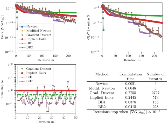
Fig. 2. Test case 1. Sum of square interpolation of ppxq “ x5` 1. (Top left) Error }∇Gpλmq}
vs. iteration m; (Top right) Objective function Gpλmq vs. iteration m; (Bottom left) Step size τm vs.
iterationm; (Bottom right) Number of iterates and computation time to reach }∇Gpλq} ă 10´8for each
method.
6.1.1. Test case 1. We compare the convergence of the methods for an easy objective polynomial, that is a polynomial with low degree and far above 0: we take n “ 5, r˚“ i˚“ n ` 1 “ 6, ppxq “ x5` 1
and the weights g1pxq “ x with g2pxq “ 1 ´ x (so j˚“ 2).
We observe on Figure2that the Newton type methods both reach the threshold precision of 10´8after
only 6 iterations. The implicit Euler and gradient descent methods need respectively 573 and 2727 iterations to reach the same error: this low convergence has been observed for many other test cases. This is why we continue the tests with the Newton and Barzilai and Borwein methods only.
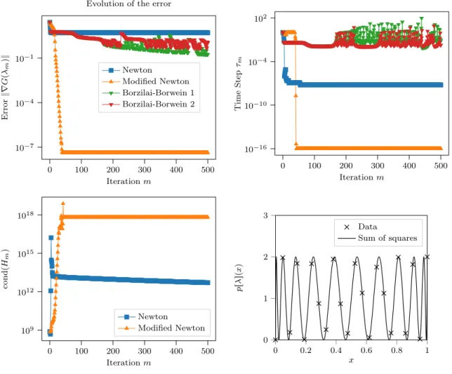
6.1.2. Test case 2. In this second test case, we illustrate the better performance of the modified Newton-Raphson method compared to the other methods. We choose a highly oscillating objective polynomial with lower bound equal to 0. It is given by n “ 21, r˚“ i˚“ n ` 1 “ 22, ppxq “ T21pxq ` 1
and the weights g1pxq “ x with g2pxq “ 1 ´ x (so j˚“ 2).
We observe on Figure3 that the modified Newton-Raphson method reaches a precision of around 10´8 in 40 iterations. In the case of the standard Newton-Raphson method, the adaptive time step
quickly reduces to a very small value in order to keep decreasing the error at each iteration. A similar phenomena happens near convergence for the modified Newton-Raphson method. These behaviors
0 100 200 300 400 500 10´7 10´4 10´1 Iteration m Error } ∇ G p λm q}
Evolution of the error
Newton Modified Newton Borzilai-Borwein 1 Borzilai-Borwein 2 0 100 200 300 400 500 10´16 10´10 10´4 102 Iteration m Time Step τm 0 100 200 300 400 500 109 1012 1015 1018 Iteration m cond p Hm q Newton Modified Newton 0 0.2 0.4 0.6 0.8 1 0 1 2 3 x p rλ sp x q Data Sum of squares
Fig. 3. Test case 2. Sum of square interpolation of ppxq “ T21pxq ` 1. (Top left) error }∇Gpλmq}2 vs. iteration m; (Top right) Step size τmvs. iteration m; (Bottom left) Condition number of Hm vs. iteration m; (Bottom right) Data pyr“ ppxrqqr and sum of squares prλspxq satisfying }∇Gpλq} ă 10´6.
can be interpreted thanks to the evolution of the condition number of the matrix Hm also showed on
Figure3. Let us recall that this matrix needs to be inverted at each iteration. On the first hand, for the Newton-Raphson method, Hmis the Hessian of G which degenerates when λ is far from the minimizer
of G, as explained in Lemma 3.11. The modified Newton-Raphson method seems to prevent a bad condition number of the tweaked Hessian in the first few iterations. On the second hand, since the objective polynomial has a 0 lower bound, strict convexity and coercivity of G are not granted and it may explain the bad conditioning of Hmnear convergence in the case of the modified Newton-Raphson
method. Indeed recall that when ∇Gpλmq is small Hmalmost coincides with the Hessian in the modified
Newton-Raphson method.
Concerning the Barzilai and Borwein methods, we found out that the convergence is very slow on this test case. A minimal error }∇Gpλmq} of around 10´4 is attained after 100000 iterations for the
“BB1” method, and worse performances are obtained with the “BB2” method. While these methods are well-suited for many nonlinear programming problems, it seems that despite the cost of the Hessian
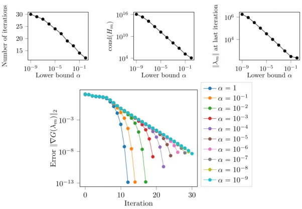
10´9 10´5 10´1 15 20 25 30 Lower bound α Num b er of iterations 10´9 10´5 10´1 104 1010 1016 Lower bound α cond pH m q 10´9 10´5 10´1 104 106 Lower bound α } λm } at last iteration 0 10 20 30 10´13 10´8 10´3 Iteration Error } ∇ G pλ m q} 2 α “ 1 α “ 10´1 α “ 10´2 α “ 10´3 α “ 10´4 α “ 10´5 α “ 10´6 α “ 10´7 α “ 10´8 α “ 10´9
Fig. 4. Test case 3. Influence of the lower bound α in the sum of square interpolation of ppxq “ pT11pxq ` 1q ` α. (Top left) Number of iterations to converge vs. α; (Top right) Condition number of Hm at the last iteration vs. α; (Bottom) Error }∇Gpλmq}2 vs. iteration m for different lower bounds α.
inversion, it is significantly cheaper in terms of computational effort to use Newton type iterations on our particular problem.
Eventually we found in many numerical experiments that, on the particular problem addressed in this paper, the modified Newton method is by far the most robust and efficient method among the ones we tested. This the reason why we only use the modified Newton-Raphson method in the following series of tests.
6.1.3. Test case 3. Now, we illustrate the influence of the lower bound of p on the convergence of the method. To proceed, we compute a sum of squares approximation of the polynomial ppxq “ T11pxq ` 1 ` α for various lower bounds α (n “ 5, r˚“ i˚“ n ` 1 “ 6, j˚ “ 2).
The results are displayed on Figure 4. We observe that the number of iterations required to reach a precision of 10´8 seems to increase proportionally with |logpαq|. The condition number of H
m and
the norm of λm at convergence decays like some negative power of α. Interestingly enough, one also
sees that the quadratic convergence of the (modified) Newton method seems to degenerate to linear convergence when α goes to 0. All these behaviors can be interpreted thanks to the results of Lemma3.5
and Lemma 3.11. We know from Lemma 3.5 that for α “ 0, p has a root x0 in r0, 1s, and thus the
coercivity of G is lost in some direction of the asymptotic cone of D (that of the Lagrange vector Lpx0q).
Thus as α Ñ 0, the minimizer λ˚
α may go to `8 in the asymptotic cone which would explain here the
explosion of the norm of λ and of the condition number of Hm as predicted by Lemma3.11and shown
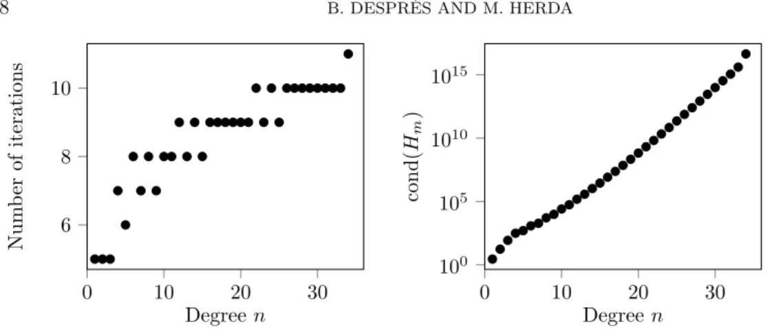
0 10 20 30 6 8 10 Degree n Num b er of iterations 0 10 20 30 100 105 1010 1015 Degree n cond pH m q
Fig. 5. Test case 4. Influence of the degree n in the sum of square interpolation of ppxq “ xn` 1. (Left) Number of iterations to converge vs. n; (Right) Condition number of Hmat the last iteration vs. n.
6.1.4. Test case 4. In this fourth test case we illustrate the influence of the degree n of the objective polynomial ppxq “ xn
` 1 on the convergence of our method, with g1pxq “ x and g2pxq “ 1 ´ x
for n odd and g1pxq “ 1 and g2pxq “ xp1 ´ xq for n even.
The result are displayed on Figure 5. We observe that the number of iterations required to reach an error of 10´8 increases with the degree, but weakly. We also observe that the condition number
condpHmq “ }Hm}}Hm´1} near convergence deteriorates with n, approximately quadratically.
6.2. Bivariate polynomials on a triangle. We use the minimization algorithm for the compu-tation of a sum of squares represencompu-tation of some positive polynomial p P PnrX, Y s on the triangle.
6.2.1. Numerical setting. The barycentric coordinates corresponding to the vertices S1, S2and
S3 of the triangle are denoted as µj for j “ 1, 2, 3: µ1px, yq “ 1 ´ x ´ y, µ2px, yq “ x and µ3px, yq “ y.
The triangle is K “ tx “ px, yq P R2
| µ1pxq ě 0 , µ2pxq ě 0 , µ3pxq ě 0u. The interpolation points
are xr“ pxr, yrq for 1 ď r ď r˚“ pn ` 1qpn ` 2q{2 are the distinct points of a cartesian grid intersected
with the triangle. For a given polynomial p P Pn
rXs of a given degree, the data is z P Rr˚ which is the
vector with components zr “ ppxr, yrq. An illustration of the geometry is provided in Figure 6 where
the degree is n “ 4.
We consider the ansatz (x “ px, yq)
(6.1) prλspxq “
rj
ÿ
i“1
g1pxq pi1rλspxq2` g2pxq pi2rλspxq2` g3pxq pi3rλspxq2` g4pxq pi4rλspxq2,
where, arbitrarily with respect to the literature [14], the weights are
(6.2)
"
for n “ 2k ` 1, gi“ µi for i “ 1, 2, 3 and g4“ µ1µ2µ3,
for n “ 2k, g1“ µ2µ3, g2“ µ3µ1, g3“ µ1µ2 and g4“ 1.
With this choice we recover in every cases r˚ “ r1` r2` r3` r4. All polynomials are parametrized on
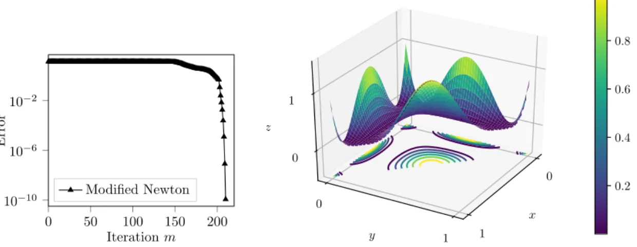
the basis of bivariate monomials since Chebychev polynomials are not available on the triangle. 6.2.2. Test case 5. We approach the polynomial ppx, yq “ pT4pxq ` 1qpT4pyq ` 1q{4 ` 10´3 on the
2D simplex with the modified Newton method. The parameters are n “ 8, r˚“ i˚“ 45 and j˚“ 4.
We observe on Figure 7 that our method converges in this multivariate setting and reaches a precision of less than 10´8 in 210 iterations. The error decays slowly during the first 200 iterations
´0.2 0 0.2 0.4 0.6 0.8 1 1.2 0 0.5 1 S1 S2 S3 x y
Domain and interpolation points
Fig. 6. The simplex K and interpolation points for n “ 4.
0 50 100 150 200 10´10 10´6 10´2 Iteration m Error Modified Newton x 0 1 y 0 1 z 0 1 0.2 0.4 0.6 0.8 1.0
Fig. 7. Test case 5. Bivariate sum of square interpolation of the degree 8 polynomial ppx, yq “ pT4pxq ` 1qpT4pyq ` 1q{4 ` 10´3on the 2D simplex. (Left) error }∇Gpλ
mq}2 vs. iteration m; (Right) surface plot of the converged sum of square.
before reaching usual quadratic speed of convergence of the Newton method near the minimizer of G. This result illustrates the ability of our algorithms to provided a computational strategy for the computation of positive polynomials on bi-dimensional sets.
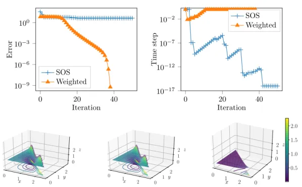
6.2.3. Test case 6. In this last test case we are interested in the SOS approximation of the Motzkin polynomial [19] ppx, yq “ x2y4
` y2x4
´ 3x2y2
` 1.
This polynomial is non-negative over R2 and famous for not being a sum of square in the sense
that it admits no decomposition (1.3) with weigthsrg1 “ ¨ ¨ ¨ “rgj˚ “ 1 (whatever the choice of i˚ or,
equivalently in this particular case, j˚). The parameters are n “ 6, r˚ “ i˚ “ 28 and j˚ “ 4. We use
our method to approach this polynomial with the sum of square ansatz (6.1) but with two different weights: on the one hand we use the weights gi (6.2) for which we expect some convergence of the
0 20 40 10´9 10´6 10´3 100 Iteration Error SOS Weighted 0 20 40 10´17 10´12 10´7 10´2 Iteration Time ste p SOS Weighted x 0 1 2 0 y 1 2 z 0 1 2 x 0 1 2 0 y 1 2 z 0 1 2 x 0 1 2 0 y 1 2 z 0 1 2 0.5 1.0 1.5 2.0
Fig. 8. Test case 6. Bivariate sum of square approximations (of degree n “ 6) of the Motzkin polynomial. (Top left) error }∇Gpλmq}2vs. iteration m; (Top right) time step τmvs. iteration m; (Bottom left) The Motzkin polynomial; (Bottom center) Sum of square approximation with weights g1“ µ2µ3, g2“ µ3µ1, g3“ µ1µ2and g4“ 1, the algorithm has converged; (Bottom right) Sum of square approximation without weights (g1“ g2“ g3“ g4“ 1), the algorithm has not converged;
In the latter case our experiment on Figure8show the method does not converge (in coherence with the non-existence of a sum of square decomposition for the Motzkin polynomial). The algorithm with weights gi converges while the algorithm with weights rgi does not converge (bottom right illustration in the Figure).
7. Concluding remarks. In this paper, we reformulated the problem of computing SOS decom-positions into a new nonlinear convex program. On the theoretical side we analyzed this reformulation in detail, and particular the domain which guarantees convexity, and showed that up to a perturbation the problem is proper strictly convex and coercive, which ensures the existence of a solution which may be explicitly approached via iterative methods. As the literature in numerical optimization is immense, we did not give an exhaustive numerical comparison of all the methods that could be used to solve our problem. Preferably, we tried to design robust methods specifically adapted to the structure of our objective function and compare it with some classical algorithms in numerical optimization. Our numerical results show that the modified Newton-Raphson algorithm is robust to compute polynomials which respect a sign condition on a given simple semi-algebraic set. However more needs to be inves-tigated to compare with different methods and evaluate the full potential of such methods. Here we detail possible domains of research which are consequences of the multiple connections of our methods with the ones of Scientific Computing.
‚ It is possible to look in more details in the case i˚ ‰ r˚. It allows greater generality of the
con-struction, which can be convenient for optimization purposes. In such cases, the function G should be replaced by GV.
needs further examinations. In this direction there may be links with algebraic properties such as the Archimedeanity of the quadratic module associated with the weights gj(see [14, proof of Theorem 2.14])
or the condition of Linear Independence Constraint Qualification (LICQ) [23].
‚ A C++ implementation needs to be tested. On this basis it will be possible to couple with codes in scientific computing (such as the ones evoked in [27] and the references therein) to evaluate the gain in robustness with the new algorithms. Comparisons with other established softwares like the primal-dual interior-point SDP Mosek-Yalmip package [17] in Matlab will be a plus. Such benchmarks are left for future work.
Appendix A. The asymptotic cone for univariate polynomials.
One can obtain a much better understanding of the cone at infinity, which exemplifies the role of the Lagrange interpolating polynomials. Given a subset S Ă Rn`1one denotes by conipSq the conical
hull of S that is the set of linear combinations with non-negative coefficients of elements of S. The asymptotic cone can be constructed from the matrices (4.4) or (4.5) in the univariate case. The main result is the following, where the the Lagrange vectors are defined in (3.2).
Theorem A.1. The asymptotic cone of D is generated by the Lagrange vectors Lpxq for 0 ď x ď 1, that is C8 “ coniptLpxq P Rn`1| x P r0, 1suq.
We need some intermediate results in order to prove TheoremA.1. First, let us define C1
8“ tλ P
C8 |
řn`1
r“1λr “ 1u Ă C8. Since
řr˚
r“1lrpxrq “ 1 for all 1 ď r ď r˚, one has
řr˚
r“1lrpXq “ 1.
Therefore, with Lemma 3.2, we know that Lpxq P Rn`1| x P r0, 1s(
Ă C81. The main point of the proof is to show that C1
8Ă Lpxq P Rn`1, | x P r0, 1s(. To do so we identify C 1
8 with a subset of Borel
probability measures on r0, 1s using the theory of the moment problem for which an comprehensive reference is [13]. The proof of the Theorem invoked below in the proof is strongly related to the Lukacs decomposition of Theorem4.1.
Proposition A.2. Let λ P Rn`1. The following are equivalents: a) The vector λ belongs to C81;
b) There is a Borel probability measureσ on r0, 1s such that
(A.1) n`1 ÿ r“1 λrBr“ ż r0,1s Bpxqdσpxq. Proof. Using (4.5), one can say that λ P C1
8 ðñ ps0, . . . , snq are such that H1 and H2are positive
semidefinite matrices and s0“ 1. By [13, Theorem 2.3, Theorem 2.4], this is equivalent to the existence
of a Borel probability measure σ such that (A.1) holds. Corollary A.3. The set C81 is compact.
Proof. Since, by PropositionA.2, the si’s are moments of a Borel probability measure on r0, 1s, one
has ps0, . . . , snq P r0, 1sn`1. Therefore, since λ ÞÑ ps0, . . . , snq is linear and invertible (see Lemma4.3),
C1
8 is bounded.
We recall that a point λ of a convex set C is said to be an extreme point (see [11, III, Definition 2.3.1]) of C if for any λ1, λ2P C such that λ “ pλ1` λ2q{2, one has λ “ λ1“ λ2. We denote by extpCq
the set of extreme points of C.
Proposition A.4. The set of extreme points of C81 isextpC 1
8q “ tLpxq | x P r0, 1su.
Proof. Let λ P extpC1
8q. Since extreme points of a convex set are located on its boundary there is
a vector V ‰ 0 such thatAřn`1
r“1λrBrV, V
E
“ 0. Let σ be a Borel measure satisfying (A.1) and define qpXq “ xBpXqV, Vy ě 0. One has ş
r0,1sqpxqdσpxq “ 0. Since q is not identically zero, the measure σ
n, σ has the form σ “řn
k“1αkδxk where
řn
k“1αk “ 1, 0 ď αk ď 1 and xk P r0, 1s, for some distinct
x1, . . . , xn and where δxk is the Dirac measure at xk. Now assume that for some index k, αk P p0, 1q.
Then there is k1 ‰ k such that α
k1 P p0, 1q. Then let 0 ď ε ă minpαk, αk1, 1 ´ αk, 1 ´ αk1q and define
σ1 “ σ ´ εδxk` εδxk1 and σ2 “ σ ` εδxk´ εδxk1. The measures σ1 and σ2 are two Borel probability
measures generating different sets of moments for at least some ε in the range. Since λ ÞÑ ps0, . . . , snq is
linear and invertible there are distinct λ1, λ2P C81 satisfying (A.1) for the respective measures σ1and σ2
and one has λ “ pλ1` λ2q{2. There is a contradiction. Therefore either αk“ 0 or αk“ 1 so σ must be a
dirac measure at some point x˚P r0, 1s. Hence
řn`1 r“1λrBpxrq “ Bpx˚q so in particular řn`1 r“1λrx k r “ xk˚
for any 0 ď k ď n which yields λ “ Lpx˚q. Conversely if λ “ Lpx˚q and λ “ pλ1` λ2q{2, then there
are probability measures σ1 and σ2such that δx˚“ pσ1` σ2q{2. Therefore σ1 and σ2 are supported at
x˚ and since they have the same mass one has δx˚ “ σ1“ σ2, so λ P extpC
1 8q.
Proof of TheoremA.1. Denote by copSq the convex hull of S, the set of linear combinations of elements of S with non-negative coefficients whose sum equals 1. By the Minkowski (or Krein-Milman) theorem [11, III, Theorem 2.3.4], any compact convex set is the convex hull of its extreme points, therefore C1 8“ copextpC 1 8qq. Remark that C8“ Ť tě0tC 1
8 and the result follows.
REFERENCES
[1] J. Barzilai and J. M. Borwein, Two-point step size gradient methods, IMA J. Numer. Anal., 8 (1988), pp. 141–148. [2] L. Beir˜ao da Veiga, A. Buffa, G. Sangalli, and R. V´azquez, Mathematical analysis of variational isogeometric
methods, Acta Numer., 23 (2014), pp. 157–287.
[3] S. Boyd and L. Vandenberghe, Convex optimization, Cambridge University Press, Cambridge, 2004.
[4] S. Burer and R. D. C. Monteiro, A nonlinear programming algorithm for solving semidefinite programs via low-rank factorization, Math. Program., 95 (2003), pp. 329–357. Computational semidefinite and second order cone programming: the state of the art.
[5] F. Charles, M. Campos-Pinto, and B. Despr´es, Algorithms for positive polynomial approximation, to appear in Siam J. Numer. Analysis, (2017). Online at https://hal.sorbonne-universite.fr/hal-01527763.
[6] B. Despr´es, Polynomials with bounds and numerical approximation, Numerical Algor., 76 (2017), pp. 829–859. [7] B. Despres and M. Herda, Correction to: Polynomials with bounds and numerical approximation, Num. Algor.,
(2017).
[8] R. A. DeVore and G. G. Lorentz, Constructive approximation, vol. 303 of Grundlehren der Mathematischen Wissenschaften [Fundamental Principles of Mathematical Sciences], Springer-Verlag, Berlin, 1993.
[9] D. di Serafino, V. Ruggiero, G. Toraldo, and L. Zanni, On the steplength selection in gradient methods for unconstrained optimization, Appl. Math. Comput., 318 (2018), pp. 176–195.
[10] D. Henrion and J. Malick, Projection methods for conic feasibility problems: applications to polynomial sum-of-squares decompositions, Optimization Methods & Software, 26 (2011), pp. 23–46.
[11] J.-B. Hiriart-Urruty and C. Lemar´echal, Convex analysis and minimization algorithms. I, vol. 305 of Funda-mental Principles of Mathematical Sciences, Springer-Verlag, 1993.
[12] M. Korda, D. Henrion, and C. N. Jones, Convergence rates of moment-sum-of-squares hierarchies for optimal control problems, Systems Control Lett., 100 (2017), pp. 1–5.
[13] M. G. Kre˘ın and A. A. Nudel’man, The Markov moment problem and extremal problems, American Mathematical Society, Providence, R.I., 1977.
[14] J. B. Lasserre, Moments, positive polynomials and their applications, vol. 1 of Imperial College Press Optimization Series, Imperial College Press, London, 2010.
[15] J. B. Lasserre, An introduction to polynomial and semi-algebraic optimization, Cambridge Texts in Applied Math-ematics, Cambridge University Press, Cambridge, 2015.
[16] B.-G. Lee, T. Lyche, and K. Mørken, Some examples of quasi-interpolants constructed from local spline projectors, in Mathematical methods for curves and surfaces (Oslo, 2000), Innov. Appl. Math., Vanderbilt Univ. Press, Nashville, TN, 2001, pp. 243–252.
[17] J. L¨ofberg, Yalmip : A toolbox for modeling and optimization in matlab, in In Proceedings of the CACSD Confer-ence, Taipei, Taiwan, 2004.
[18] J. Malick, A dual approach to semidefinite least-squares problems, SIAM J. Matrix Anal. Appl., 26 (2004), pp. 272– 284.
[19] T. S. Motzkin, The arithmetic-geometric inequality, Inequalities (Proc. Sympos. Wright-Patterson Air Force Base, Ohio, 1965), (1967), pp. 205–224.