IdEP Econom ic Papers
2015 / 06
M. Filippini, B. Hirl, G. Masiero
Rational habits in residential electricity demand
M. Filippini 1 B. Hirl 2 G. Masiero 3
November 2015
Abstract
Dynamic partial adjustment models of residential electricity demand account for the fact that households may not adjust electricity consumption immediately in response to changes in prices, income, and other relevant factors, because of behavioral habits or adjustment costs for the capital stock of appliances. How-ever, forward-looking behavior is generally neglected. Expectations about future prices or consumption may have an impact on current decisions. In this paper we propose rational habit models for residential electricity demand and apply them to a panel of 48 US states between 1995 and 2011. We estimate lead consumption models using fixed effects, instrumental variables, and the GMM Blundell-Bond estimator. We find that expectations about future consumption significantly in-fluence current consumption decisions, which suggests that households behave rationally when making electricity consumption decisions. This novel approach may improve our understanding of the dynamics of residential electricity demand and the evaluation of the effects of energy policies.
JEL classification: D12, D84, D99, Q41, Q47, Q50
Keywords: Residential electricity, Partial adjustment models, Dynamic panel data models, Rational habits
1
Institute of Economics (IdEP), Università della Svizzera italiana (USI); Department of Manage-ment, Technology and Economics, ETH Zurich, Switzerland.
2
Institute of Economics (IdEP), Università della Svizzera italiana (USI). Corresponding author. E-mail address: [email protected].
3
Department of Management, Information and Production Engineering (DIGIP), University of Bergamo, Italy; Institute of Economics (IdEP), Università della Svizzera italiana (USI), Switzerland.
1
Introduction
In the US, residential electricity consumption accounts for about a third of total elec-tricity consumption. Understanding the dynamics of household energy consumption is of great importance in formulating policies to improve the efficient use of energy services.
Households use energy services (e.g. lightning, TV entertainment, cooling of food, hot water) by combining electrical appliances and electricity. Therefore, households face simultaneous consumption and investment decisions: how much energy to con-sume and what stock of electrical appliances to hold. Households’ reaction to a chang-ing environment, such as an increase in the price of electricity, may then lead to an adjustment in the stock of electrical appliances or a change in their use. For in-stance, households may decide to switch to a more energy efficient lightning system, or they may adjust their consumption habits by switching off the light more often when leaving a room.
Rational households, looking at the constant maximization of utility over time (Becker and Murphy, 1988), take expectations about future electricity consumption or prices into account when making current consumption and investment decisions. In addition, because of habits or the constraint generated by the opportunity cost of changing the stock of electrical appliances, current consumption decisions are affected by past consumption. Households may not be able to change their electricity consump-tion or to adjust their stock of electrical appliances immediately to react to changes in the price of electricity. Therefore, households’ current consumption depends on both past and future consumption levels.
The recent literature on residential electricity demand neglects rational households behavior (e.g., Alberini and Filippini, 2011; Blázquez et al., 2013; Cebula, 2012). Generally, residential electricity demand is estimated using static models, where no interdependence of consumption decisions over time is assumed, or using dynamic partial adjustment models that account only for the impact of past consumption. To our knowledge, only one study considers rational habits in energy consumption (Scott, 2012), but the analysis focuses on gasoline rather than electricity, and the econometric approach relies on lead price models, i.e. models where current consumption is affected by future prices, rather than lead consumption models, i.e. models where current and future consumption are interdependent.
This paper builds on the literature on rational habits (e.g., Becker et al., 1994) to extend and generalize the existing dynamic partial adjustment approach to electricity
demand by considering expectations about future consumption. This novel approach can provide more precise estimates of the dynamics of residential electricity consump-tion due to behavioural habits and constraints in the stock of appliances. We show that expectations about changes in future consumption significantly influence current consumption, which suggests evidence of rational household behavior in electricity consumption decisions.
The remaining of the paper is organized as follows. Section 2 gives an overview of the existing literature on residential electricity consumption. In section 3 we derive a rational habit model of residential electricity consumption. Section 4 presents the empirical approach and describes the data, and section 5 discusses the econometric estimation. The results are summarized and discussed in section 6. Section 7 concludes the paper.
2
Residential electricity demand in the literature
Residential electricity demand has been studied extensively in the economic literature. Since the early works of Houthakker (1951), Fisher and Kaysen (1962) and Mount et al. (1973), the focus of most studies has been the relationship between price and consumption, using rather similar sets of control variables (electricity prices, prices of substitutes, income, weather and climate conditions). First empirical studies on energy demand were based on aggregate data sets (state or city level), whereas studies published in the eighties and afterwards made use of aggregate as well as disaggregate data sets. In this review of the literature, we are mainly interested in studies based on aggregate data sets.1
More recent studies largely vary in the estimated short- and long-run price elastic-ities. These differences are likely due to different time periods, data sets (time series vs. panel data) and econometric approaches. Okajima and Okajima (2013) and Espey and Espey (2004) give an overview of estimated short- and long-run price and income elasticities. Short- and long-run price elasticities of selected studies of residential elec-tricity demand from different geographic regions are summarized in Table 1. Price elasticitites vary between -0.05 and -0.4 in the short-run, and between -0.19 and -1.89 in the long-run.
Regarding the econometric approach, most studies employ either static models or dynamic partial adjustment models. Static residential electricity demand models are usually estimated using ordinary least squares (OLS) and fixed effects (FE) or
1
A comprehensive survey of early studies on electricity demand with a focus on the residential sector is provided by Taylor (1975) and Bohi and Zimmerman (1984).
random effects (RE) models. Eskeland and Mideksa (2009) estimate a static model for residential electricity demand in 31 European countries. The main interest of the authors lies on the impact of temperature changes on electricity consumption. Also, Azevedo et al. (2011) estimate residential electricity demand using static models applied to two panels: 1990-2003 for 15 EU countries, and 1990-2004 for US states. The authors find shortrun price elasticities of 0.2 for the EU15, and 0.21 to -0.25 for the US. More recently, Cebula (2012) estimates residential electricity demand using US state-level data between 2002 and 2005. The emphasis of this study is on the key influencing factors of residential electricity consumption and the impact of state energy efficiency policies. Through a two-stage least squares approach, the author estimates that residential electricity consumption decreases with the adoption of energy efficiency programmes. Furthermore, electricity consumption decreases with price, and increases with annual cooling degree days and per capita real disposable income.
Dynamic partial adjustment models are generally more realistic than static models and allow for the calculation of short- and long-run prices and income elasticites. Early studies by Houthakker et al. (1974) and Houthakker (1980) estimate price elasticities at the national and regional level allowing for a partial adjustment in consumption. More recently, Bernstein and Griffin (2006) and Paul et al. (2009) employ dynamic models for energy demand, although they do not address the potential dynamic panel bias that arises by including the lag of consumption. Both studies estimate residential electricity demand in the US. The former study uses data between 1977 and 2004, and finds short- and long-run price elasticities of -0.24 and -0.32 respectively. The latter study covers the years 1990 to 2004, and estimates short-run price elasticities between -0.11 and -0.15. The authors claim that attempts to instrument the lag of consumption using past prices and demand did not succeed, and resulted in unstable estimates. Therefore, only least squares dummy variable (LSDV) estimates are reported.
Some recent studies account for dynamic panel bias and use more advanced dy-namic panel data models (e.g., panel cointegration, autoregressive distributed-lag (ARDL), generalized method of moments (GMM) estimators) or corrected FE models (e.g., Kiviet (1995) estimator). Dergiades and Tsoulfidis (2008) investigate residen-tial electricity demand in the US between 1965 and 2006 using the ARDL approach to panel cointegration. They estimate a short-run price elasticity of -0.39, and a long-run elasticity of -1.07. Bernstein and Madlener (2011) analyze residential elec-tricity demand for 18 OECD countries over the time period 1981-2008 using panel cointegration and Granger causality testing. They find a short-run price elasticity of
-0.1, and a long-run elasticity of -0.39. Lower values (-0.07 and -0.19) are obtained by Blázquez et al. (2013), who apply a FE estimator and the Blundell-Bond system GMM estimator to a Spanish panel. Alberini and Filippini (2011) estimate dynamic models of residential electricity in the US and obtain slightly larger elasticities: be-tween -0.08 and -0.15 for the short-run, and bebe-tween -0.44 and -0.73 for the long-run. The Kiviet corrected FE estimator and the system Blundell-Bond GMM estimator are used to account for possible correlation between the lag of consumption and the error term. To tackle possible endogeneity of electricity price due to measurement error, the authors also consider an instrumental variable approach.2 Finally, Kamer-schen and Porter (2004) use both a partial adjustment approach and a simultaneous equation approach. Simultaneous equation models provide negative price elasticities, whereas partial adjustment models provide positive price elasticities in some cases. The authors conclude that partial adjustment models are more appropriate in the case of energy demand estimation.
To our knowledge, none of the studies in the above literature on residential elec-tricity demand considers expectations about future prices or consumption. A recent study by Scott (2012) represents a partial exception since it focuses on gasoline de-mand. The author estimates rational habit models for gasoline demand in the US including expectations about gas prices. However, the empirical approach includes the lead of price as explanatory variable instead of the lead of consumption suggested by the theoretical model used in this paper. In our empirical analysis of residen-tial electricity demand in the US, we estimate rational habit models that include both past and lead consumption as explanatory variables in accordance with the theoretical approach proposed by Becker et al. (1994).
3
A rational habit model of residential electricity demand
In this section, we build a rational habit model of residential electricity consump-tion by extending and generalising the existing dynamic partial adjustment model. Households are assumed to maximize utility from energy services based on electricity (e.g. lighting, hot water, cooling, and entertainment) and other consumption goods. Energy services can be produced by combining two inputs: electricity and electrical appliances.2Another possibility to account for potential endogeneity of price is to employ simultaneous equa-tion models. However, Baltagi et al. (2002) and Baltagi (2007) find that generalized least squares (GLS), FE, and OLS estimation techniques outperform the simultaneous equation approach in most cases.
Household utility at time t is then given by:
Ut= u(et, At, ct; xt), (1)
where et is electricity, At is the capital stock of electrical appliances, ct represents all other consumption goods, and xt is a vector of other (environmental) variables affecting the consumption of energy services, such as weather and energy substitutes.
Using Eq. (1) we can write the lifetime utility function of the household as:
∞ X t=1 δt−1Ut= ∞ X t=1 δt−1u(et, At, ct; xt), (2)
where δ = (1 + r)−1 is the constant rate of time preference and r is the interest rate. We hypothesize that the stock of electrical appliances is the accumulation of elec-tricity investments over time, which can be approximated by past elecelec-tricity use. Therefore, the current stock electrical appliances develops according to the following relationship:
At= (1 − ρ)At−1+ et−1, (3)
where ρ is the depreciation rate of the stock, i.e. the rate at which electrical appliances lose their ability to provide satisfactory energy services in the absence of energy in-vestments. Because this stock adjustment condition relates the stock of appliances to the consumption of electricity, we can see the stock of electrical appliances as a stock of behavioural habit. Agents are habituated to some use of energy, which generates a stock of behavioural habit to electricity consumption.
Using Eqs. (2) and (3) we can write the household lifetime utility maximization problem. To simplify the analysis we assume that the stock of habit fully depreciates after one period, i.e. ρ = 1. Consequently, we get:
∞ X t=1 δt−1u(et, et−1, ct; xt) (4) s.t. e0 = E0 and ∞ X t=1 δt−1(ct+ Ptet) = W0, (5)
where E0is the initial condition defining the level of electricity consumption in period 0, W0 is the present value of wealth, and Pt is electricity price at period t.
The first-order conditions to solve the problem above imply that the marginal utility of current electricity consumption plus the discounted marginal effect on the next period’s utility of current consumption is equal to the marginal utility of wealth multiplied by the current electricity price. Furthermore, the marginal utility of wealth
equals the marginal utility of the composite good in each period. Using a quadratic utility function, the solution of the order conditions leads to the following first-difference equation:
et= θet−1+ δθet+1+ θ1Pt+ θ2xt+ δθ3xt+1. (6)
In this equation current electricity consumption is a function of past and future con-sumption, price, and all other variables, some of which are unobserved. The coefficient θ depends on the parameters of the quadratic utility function.3 Expectations about environmental conditions, such weather or price of energy substitutes, are captured by the coefficient of xt+1.
4
Empirical model and data
To empirically investigate the dynamics of residential electricity consumption, we modify the first-difference equation (6) to obtain:4
eit = β0+ β1eit−1+ β2eit+1+ β3Pit+ β4P Git+ β5Yit+ β6HDDit+
+β7CDDit+ β8HSit+ vit, (7)
where eit is residential electricity consumption in the ith state (i = 1, ..., 50) at time t, P Git is the price of electricity substitutes (gas), Yit is income per capita, HDDit and
CDDit denote, respectively, heating degree days and cooling degree days, and HSit
is the household size. The remaining unobserved variables may be time-invariant or time-variant. Time-invariant aspects are captured by fixed-effects estimators in our econometric approach (see section 5). The residual time-variant unobserved hetero-geneity is included in the disturbance term vit.
The coefficient β1 captures the impact of past consumption on current
consump-tion. Consequently, a positive and significant coefficient is consistent with the hy-pothesis that electricity consumption is a habit. Moreover, the rational habit model defined by Eq. (7) allows us to capture the behaviour of forward-looking agents. How agents adjust their current consumption in response to expectations on future consumption sheds light on rational behaviour. Rational households are expected to increase current consumption in anticipation of higher consumption in the future. The coefficient β2 measures the impact of future consumption on current consumption. A
positive and significant coefficient would be consistent with the hypothesis of rational
3
For further details see Baltagi and Griffin (2001). A comprehensive discussion on the interpre-tation and derivation of Eq. (6) can be found in Becker et al. (1994).
behaviour and would support rejecting the hypothesis of myopic behaviour, which is implicit in partial adjustment models of electricity demand. From Eq. (7) we can also obtain the rate of time preference (δ) as the ratio between the estimated coefficient of eit+1 (β2) and the estimated coefficient of eit−1 (β1).
Short- and long-run price elasticities can be obtained from Eq. (7). We can expect that electricity demand in the short run is less responsive to price changes than in the long run, as the stock of electrical appliances or behavioural habits concerning electricity consumption cannot be changed immediately. Indeed, some habits such as switching off the lights when leaving a room, can be changed quickly in response to rising electricity prices. Other habits can be more persistent, for instance TV view-ing time per day. Moreover, the replacement of most electrical appliances for more efficient ones represents a considerable financial investment for the majority of house-holds. Therefore, we cannot expect immediate replacement in response to changing prices, and short-run electricity consumption may depart from long-run optimal con-sumption. The demand does not adjust immediately to the long-run equilibrium, but gradually converges to the optimum level even when consumers are rational and have expectations about future electricity demand.
Static models of electricity consumption can be derived from our rational habit model. In the static case, there is no delay in the adjustment process since there is no link between consumption in different periods. Static models assume that there are no costs of adjustment nor expectations that affect current decisions. The tradi-tional dynamic partial adjustment model is more realistic as it allows for the sluggish adjustment process between optimal (long-run) consumption levels and short-run con-sumption. This model can be obtained from Eq. (7) assuming that agents do not take information about the future into account. Therefore, households appear to be my-opic. Myopic households maximize current period utility instead of the lifetime utility function (2) under the assumption that current electricity consumption is affected by past consumption as hypothesized by Eq. (3). Finally, our full empirical model may disclose evidence of rational habits in residential electricity consumption if households take into account expectations about the future when making current consumption decisions.
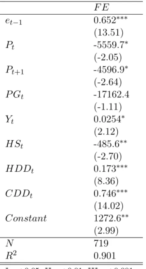
An alternative to the lead consumption model (7) is to define a lead price model, which assumes that future prices represent the relevant information for rational con-sumers. This empirical approach builds on the theoretical model developed by Brown-ing (1991), who defines a demand system for many goods startBrown-ing from intertemporal nonseparability in preferences. Inspired by this work, Scott (2012) estimates a
lead-price rational habit model for gasoline demand based on a single equation and using a log-log functional form. Since the theoretical framework fails to derive closed-form, analytical solutions, the author uses simulation to discuss the model implications. Consequently, the parameters of the suggested empirical model cannot be interpreted straightforwardly using the theoretical model. In the following empirical analysis we will focus on lead consumption models, which derive directly from our theoretical framework.5
4.1 Data
To test the hypothesis of rational behaviour in the consumption of residential elec-tricity, we use a data set covering 51 US states (including the District of Columbia) from 1995 to 2011. For the analysis, three states (Alaska, Hawaii, and Rhode Island) are excluded because of incomplete observations. Descriptive statistics for electricity consumption and prices, and other important covariates for the remaining 48 states are presented in Table 2.
Data on residential electricity consumption (e), electricity price (P ) and gas price (P G) are provided by the US Energy Information Agency (EIA). The average electric-ity and gas prices are obtained by dividing utilities revenues by sales in the residential sector (EIA calculation). Information on income (Y ), number of inhabitants in the state (P OP ) and the number of housing units necessary to calculate average house-hold size (HS = P OP /housing units), are from the Bureau of Economic Analysis of the US Census Bureau. Heating degree days (HDD) and cooling degree days (CDD) are obtained from the National Climatic Data Center at the National Oceanic and Atmospheric Administration (NOAA).6
The box-and-whiskers graph (Figure 1) shows the variation in residential electric-ity consumption across states over time. Residential electricelectric-ity consumption slighly increases over time. We observe that the variation within states (between variation) largely overcome the variation over time (within variation).7 The increasing trend in residential electricity consumption is associated to a decrease in price in the first half of the period. Conversely, during the second half of the period residential electricity
5
Some results from the estimation of a lead price model are reported in the Appendix (Table 7). 6Degree day is an index that reflects demand for energy to heat or cool houses. The index is obtained from daily temperature observations at major weather stations in the US. Heating (cooling) degree days are summations of negative (positive) differences between the mean daily temperature and the 65◦F base during a year.
7In the box and whiskers plot the horizontal line inside the shaded box represents the mean consumption of residential electricity across states in each year. The width of the shaded box includes consumption in the second quartile, i.e. 50% of the states in a given year. Finally, the length of the two whiskers illustrates the third quartile of observations, i.e. 75% of the states.
price increased.
As we will discuss in more detail later, instrumental variables for the lead and the lag of consumption as well as for the prices are needed to estimate our model (7). For a preliminary investigation of potential instruments, Table 3 shows cross-correlations between residential electricity consumption (et), price of residential electricity and gas (Pt and P Gt), lead electricity price (Pt+1) and spatial lag of electricity price (P−i,t), and price of gas and coal for the energy production sector (P Gpt and P C
p t).
Also, Figure 2 provides a graphical illustration of some price figures. The spatial lag of electricity price is calculated as the average price of bordering states for each state included in the data set. Some of these figures are clearly of interest as external instruments for the lead of consumption and electricity prices in our lead consumption models.
5
Econometric approach
For the estimation of the electricity demand equation (7), we have a balanced panel data set for 48 US states observed over the period 1995 to 2011. Therefore, the data set is characterized by a relatively long time dimension (T= 17) and a relatively small number of units (N=48). In the choice of the estimator for the dynamic model we should consider three potential econometric problems. First, due to the relatively low number of explanatory variables, a possible unobserved heterogeneity bias could be present. Second, the lagged and lead electricity consumption could be endogenous and create the so called “dynamic panel bias” (Nickell, 1981; Roodman, 2009). This bias arises because the lagged and lead dependent variable are positively correlated with the unobserved fixed effects. Since the individual fixed effects are part of the error terms in all periods, et−1and et+1 will be correlated with the current error term. Third, as discussed in Alberini and Filippini (2011), the electricity price variable could suffer from a measurement error problem. This measurement error could be due to the fact that electricity price has been calculated by the US Energy Information Agency by dividing the total revenue from sales in the residential sector by total kWh sold to residential customers.
Generally, to account for unobserved heterogeneity bias using panel data, we can specify models with either fixed effects (FE) or random effects (RE). Further, to solve the endogeneity problem of some of the explanatory variables we can use a two-stage least squares (2SLS) estimator or estimators based on a the general method of moments (GMM). Arellano and Bond (1991) as well as Blundell and Bond (1998) propose two different estimators based on GMM. For instance, Blundell and Bond
(1998) propose a system GMM estimator (GMM-BB), which uses lagged first differ-ences as instruments for equations in level as well as the lag variable in first-difference equations. However, as discussed by Baltagi et al. (2002), one possible problem of these two GMM estimators is that their properties hold for N large, so the estimation results can be biased in panel data with a small number of cross-sectional units as in our case.8
In this study, we choose to estimate model (7) using the following three estimators: FE, 2SLS fixed effects (FE2SLS) and the two-step system GMM estimator proposed by Blundell and Bond (1998).9 The FE and GMM estimators are used for comparison purposes. Note that Baltagi and Griffin (2002) and Filippini and Masiero (2011) have successfully applied the FE2SLS estimator in dynamic demand models that include both lead and lagged values of consumption as explanatory variables. In this approach, lagged and lead values of prices, income and other covariates are used as instruments for past and future consumption. One of the advantage of the FE2SLS estimator is that it can be also used with a relatively small N.
The battery of instruments used in our estimations is quite generous. The instru-ments used in the FE2SLS model are the one- and two-period lags and future values of the spatial lag of electricity price, the input prices of coal and gas for the electricity sector, and the one-period lag and lead of heating degree days. To be a valid instru-ment, the variable has to be correlated with the regressors and uncorrelated with the error term. We are instrumenting three regressors: the lag of electricity consumption, the lead of electricity consumption, and the price of electricity. The price of electric-ity is largely determined by the generation costs of electricelectric-ity. In the US, the main inputs for electricity generation are coal and natural gas. In 2014, coal and natural gas accounted for 39% and 27% of total US electricity generation, respectively. The input prices for coal and gas are the main determining factors for generation costs. The other major generation source, nuclear energy, accounts for around 19% of to-tal electricity generation. However, production costs for nuclear electricity do not change considerably over time and, therefore, are not suitable as instruments. Coal and natural gas input prices for the power generation sector have no direct influence on residential electricity consumption. Hence, they are expected to be uncorrelated with the error term of our model. Furthermore, we take the first and the second lag and lead of the spatial lag of electricity price as instruments. The spatial lag of
elec-8
For a general presentation and discussion of the estimators for dynamic panel models, see Baltagi et al. (2002).
9
In a preliminary analysis we also explored the possibility to use the corrected version of the fixed effects estimator proposed by Kiviet (1995). However, this estimator is not suitable in the presence of several endogenous variables.
tricity price represents an obvious instrument since the average of prices generated in neighbouring states is likely to be exogenous to electricity consumption within the state. Therefore, to instrument both lag and lead of consumption, we use the first lag and lead of the spatial lag of electricity price (direct effect) as well as the second lag and lead of the spatial lag of electricity price (indirect effect through past and future consumption). To account for changing weather conditions that may have an important impact on residential electricity consumption, we also include the lag and lead of heating degree days. Finally, for our GMM estimation we use the lagged values of electricity consumption and price and their first differences, the input prices of coal and gas for the electricity sector, the spatial lag of electricity price and heating degree days as well as their one- and two-period lags.
6
Estimation Results
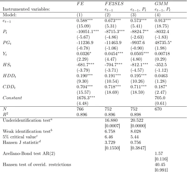
We estimate Eq. (7) using the fixed effects estimator, the system GMM estimator and two FE2SLS specifications. As previously mentioned, GMM estimators might not be suitable since we have a relatively small number of cross-sectional observations (N small), which may lead to biased results. This potential bias arises because of possible serial correlation of the idiosyncratic error term in system GMM specifica-tions. Therefore, due to the potential problems of the GMM estimator and although our results are quite robust across different specifications, the FE2SLS estimator is our preferred estimation method. To control for potential endogeneity of electricity price, we also estimate the FE2SLS model by instrumenting the price as well as the lag and lead of consumption. The estimation results of the full dynamic models of residential electricity demand are summarized in Table 4. For comparison purposes, we also provide the results of the partial adjustment model in the Appendix (Table 6).
The estimated coefficients of the lag and lead of consumption have the expected positive sign and are highly significant in all estimation approaches. The values of the coefficients are fairly robust across all estimation methods, and vary between 0.422 and 0.483 for the lag and between 0.206 and 0.374 for the lead. These results indi-cate that households are taking into account both past consumption and expectations about future consumption in their current consumption decisions. This suggests that households are not myopic and seems to disagree with the specification of the tradi-tional dynamic partial adjustment model. Although current electricity consumption is partially driven by past consumption, there is evidence that expectations about future consumption play a role in habit formation.
The coefficient of electricity price is negative and significant in all estimations. Income has a positive effect on current electricity consumption. The coefficient of the price of gas exhibits a negative sign in the FE and the FE2SLS estimations, although it is never significant. This might indicate that gas is not a good substitute for electricity. The main energy service produced with gas or electricity - room heating - is a long-run decision and, therefore, may not be affected by variations in current prices. The coefficients of heating and cooling degree days are highly significant and have a positive effect in all the estimations. This indicates that the use of electricity increases if there is more need to heat or cool the house. Finally, the coefficient of the size of the household is negative and significant, except in the GMM estimation.
For the system GMM estimation, we report the Arrelano-Bond test for serial cor-relation of the idiosyncratic error term and the Hansen test of overidentifying restric-tions. The result of the Hansen test shows that we cannot reject the null hypothesis of joint validity of the moment conditions (p-value of 0.52), suggesting that the instru-ments used are exogenous (i.e. uncorrelated with the error term) and the excluded instruments are correctly excluded. The null hypothesis of no serial correlation of the idiosyncratic error term can be rejected at the 10% level of significance (p-value of 0.087).
To test the validity of the FE2SLS estimation, we report several test statistics. The underidentification test shows that the model is identified (we reject the null hypothesis of underidentification with a p-value of 0.0000). To exclude the possibility of weak identification, we report the Kleibergen-Papp rK Wald F statistic for weak identification, and the 5% critical value. We furthermore provide the Hansen J statistic as overidentification test for the instruments used. A rejection of the null hypothesis of joint validity would cast doubt on the validity of the instruments. The Hansen J statistic is consistent in the presence of heteroskedasticity. For both FE2SLS models we cannot reject the null hypothesis of joint validity with a p-value well above 0.1. We can therefore conclude that our preferred estimation strategy (FE2SLS) passes all the relevant tests.
From Eq. (7) we can obtain short- and long-run price elasticities (εt and ε∞)
of electricity demand. These are evaluated at the means of the data (e and P ) and can be calculated using the formulas derived by Becker et al. (1994). The effect on current consumption of a permanent reduction in electricity price, i.e. the short-run elasticity, is given by εt= (det/dPt)(P/e) with det/dPt= 2β3/[1−2β2+(1−4β1β2)0.5].
The long-run effect of a permanent reduction in electricity price on consumption is measured by ε∞ = (de∞/dP )(P/e) with de∞/dP = β3/(1 − β1− β2). Similarly, we
can calculate short- and long-run income elasticities using the above formulas and substituting β3 for β5 and P/e for Y /e. When consumers are not forward-looking, as
in the traditional partial adjustment model, we can use these formulas assuming that β2 is zero.
Table 5 reports the short- and long-run price elasticities calculated for all the es-timation strategies. Short-run price elasticities in rational habit models range from 0.1077 in the FE2SLS model to 0.2708 in the GMM specification, whereas long-run price elasticities range from 0.2087 (FE2SLS) to 0.7355 (GMM). Our calculated elas-ticities are fairly robust across all models and are in line with elaselas-ticities found in the literature. Overall, we can argue that residential electricity demand is relatively inelastic in the short-run. This is probably due to the cost of adjusting immediately the stock of electrical appliances in response to a change in the price or to behavioural habits in the use of electricity. Conversely, residential electricity demand is more elas-tic to price changes in the long run. Agents have more opportunities to adapt their behavioural habits and replace their electrical equipment.
7
Conclusions
The understanding of factors affecting residential electricity demand and its respon-sinevess to price changes is of relevance to design effective energy saving policies. So far, residential electricity demand has been investigated by means of dynamic par-tial adjustment models, making restrictive assumptions on the behaviour of economic agents. Our empirical analysis suggests that the traditional dynamic partial adjust-ment model is not sufficient to explain households’ behaviour in energy consumption. This model assumes that agents do not take into account expectations about future consumption or prices when taking current consumption decisions. We provide evi-dence that agents are forward looking when choosing electricity services to maximize intertemporal utility. Therefore, partial adjustment models may lead to biased esti-mations of the impact of energy policies that change the price of electricity or have an impact on future consumption. Indeed, the current effect of policies may depend on their impact on future consumption. In other words, their effect can be reinforced by an anticipated effect on future consumption. Conversely, temporary policies that are not expected to have permanent effects on future consumption may have a negligible impact on current consumption decisions.
References
Alberini, A. and Filippini, M.: 2011, Response of residential electricity demand to price: The effect of measurement error, Energy Economics 33(5), 889–895.
Arellano, M. and Bond, S.: 1991, Some tests of specification for panel data: Monte carlo evidence and an application to employment equations, The review of economic studies 58(2), 277–297.
Azevedo, I. M. L., Morgan, M. G. and Lave, L.: 2011, Residential and regional elec-tricity consumption in the U.S. and EU: how much will higher prices reduce CO2 emissions?, The Electricity Journal 24(1), 21–29.
Baltagi, B. H.: 2007, On the use of panel data methods to estimate rational addiction models, Scottish Journal of Political Economy 54(1), 1–18.
Baltagi, B. H., Bresson, G. and Pirotte, A.: 2002, Comparison of forecast performance for homogeneous, heterogeneous and shrinkage estimators: Some empirical evidence from US electricity and natural-gas consumption, Economics Letters 76(3), 375– 382.
Baltagi, B. H. and Griffin, J.: 2001, The econometrics of rational addiction: the case of cigarettes, J Bus Econ Stat 4(19), 449–454.
Baltagi, B. H. and Griffin, J.: 2002, Rational addiction to alcohol: panel data analysis of liquor consumption, Health Economics (11), 485–491.
Becker, G. S., Grossman, M. and Murphy, K. M.: 1994, An empirical analysis of cigarette addiction, Technical report, National Bureau of Economic Research. Becker, G. S. and Murphy, K. M.: 1988, A theory of rational addiction, The journal
of political economy pp. 675–700.
Bernstein, M. A. and Griffin, J. M.: 2006, Regional differences in the price-elasticity of demand for energy, National Renewable Energy Laboratory.
Bernstein, R. and Madlener, R.: 2011, Responsiveness of residential electricity demand in OECD countries: a panel cointegration and causality analysis, Technical report, E. ON Energy Research Center, Future Energy Consumer Needs and Behavior (FCN).
Blázquez, L., Boogen, N. and Filippini, M.: 2013, Residential electricity demand in Spain: New empirical evidence using aggregate data, Energy Economics 36, 648– 657.
Blundell, R. and Bond, S.: 1998, Initial conditions and moment restrictions in dynamic panel data models, Journal of econometrics 87(1), 115–143.
Bohi, D. R. and Zimmerman, M. B.: 1984, An update on econometric studies of energy demand behavior, Annual Review of Energy 9(1), 105–154.
Browning, M.: 1991, A simple nonadditive preference structure for models of house-hold behavior over time, Journal of Political Economy pp. 607–637.
Cebula, R. J.: 2012, US residential electricity consumption: the effect of states’ pursuit of energy efficiency policies, Applied Economics Letters 19(15), 1499–1503.
Dergiades, T. and Tsoulfidis, L.: 2008, Estimating residential demand for electricity in the United States, 1965–2006, Energy Economics 30(5), 2722–2730.
Eskeland, G. S. and Mideksa, T. K.: 2009, Climate change and residential electricity demand in europe, Available at SSRN 1338835 .
Espey, J. A. and Espey, M.: 2004, Turning on the lights: A meta-analysis of residen-tial electricity demand elasticities, Journal of Agricultural and Applied Economics 36(1), 65–82.
Filippini, M. and Masiero, G.: 2011, An empirical analysis of habit and addiction to antibiotics, Empirical economics 42(2), 471–486.
Fisher, F. M. and Kaysen, C.: 1962, The demand for electricity in the united states, Amsterdam: NorthHolland .
Houthakker, H. S.: 1951, Some calculations on electricity consumption in Great Britain, Journal of the Royal Statistical Society. Series A (General) 114(3), 359– 371.
Houthakker, H. S.: 1980, Residential electricity revisited, The Energy Journal 1(1), 29–41.
Houthakker, H. S., Verleger, P. K. and Sheehan, D. P.: 1974, Dynamic demand anal-yses for gasoline and residential electricity, American Journal of Agricultural Eco-nomics 56(2), 412–418.
Kamerschen, D. R. and Porter, D. V.: 2004, The demand for residential, industrial and total electricity, 1973–1998, Energy Economics 26(1), 87–100.
Kiviet, J. F.: 1995, On bias, inconsistency, and efficiency of various estimators in dynamic panel data models, Journal of Econometrics 68(1), 53–78.
Maddala, G. S., Trost, R. P., Li, H. and Joutz, F.: 1997, Estimation of short-run and long-run elasticities of energy demand from panel data using shrinkage estimators, Journal of Business & Economic Statistics 15(1), 90–100.
Mount, T., Chapman, L. and Tyrrell, T.: 1973, Electricity demand in the United States: an econometric analysis, Amsterdam: NorthHolland .
Narayan, P. K., Smyth, R. and Prasad, A.: 2007, Electricity consumption in G7 countries: A panel cointegration analysis of residential demand elasticities, Energy policy 35(9), 4485–4494.
Nickell, S.: 1981, Biases in dynamic models with fixed effects, Econometrica 49(6), 1417.
Okajima, S. and Okajima, H.: 2013, Estimation of Japanese price elasticities of resi-dential electricity demand, 1990–2007, Energy Economics 40, 433–440.
Paul, A., Myers, E. and Palmer, K.: 2009, A partial adjustment model of US electricity demand by region, season, and sector, Resource for the Future. (DP-08-50).
Roodman, D.: 2009, How to do xtabond2: An introduction to difference and system GMM in stata, Stata Journal 9(1), 86.
Scott, K. R.: 2012, Rational habits in gasoline demand, Energy Economics 34(5), 1713–1723.
Taylor, L. D.: 1975, The demand for electricity: A survey, The Bell Journal of Eco-nomics 6(1), 74.
Tables and Figures
Table 1: Short- and long-run price elasticies of residential electricity demand from panel data models.
Study Time period Country Price elasticities
Short-run Long-run
Fisher and Kaysen (1962) 1937-1938 US -0.16 to -0.24
Houthakker and Taylor (1970) 1946-1957 US -0.13 -1.89
Mount et al. (1973) 1960-1071 US -0.14 -1.20
Maddala et al. (1997) 1970-1990 US -0.28 to -0.06 -0.87 to 0.24
Bernstein and Griffin (2006) 1977-2004 US -0.24 -0.32
Narayan et al. (2007) 1978-2003 G7 -0.11 -1.45 to -1.56
Dergiades and Tsoulfidis (2008) 1956-2006 US -0.39 -1.07
Paul et al. (2009) 1990-2004 US -0.15 to -0.11
Eskeland and Mideksa (2010) 1994-2005 Europe -0.2
Nakajima (2010) 1975-2005 Japan -1.13 to 1.20
Azevedo et al. (2011) 1990-2004 US -0.21 to -0.25
1990-2003 EU-15 -0.20 to -0.21
Bernstein and Madlener (2011) 1981-2008 OECD -0.05 to -0.06 -0.39
Alberini and Filippini (2011) 1995-2007 US -0.08 to -0.15 -0.44 to -0.73
Blázquez et al. (2013) 2000-2008 Spain -0.07 -0.19
Okajima and Okajima (2013) 1990-2007 Japan -0.4 -0.49
Table 2: Summary statistics of main variables for the whole panel (1995-2011).
Label Variable description Mean Std. Dev. Min. Max.
e Electricity consumption per capita (in kWh) 4612.931 1229.059 2147.104 7425.204
P Electicity price (per kWh) 0.049 0.013 0.03 0.095
PG Gas price (per thousand BTU) 0.005 0.001 0.003 0.01
Y Income per capita (in US $) 15227.339 2641.341 10239.206 29294.364
HDD Heating degree days 5137.783 2012.525 555 10745
CDD Cooling degree days 1142.414 803.909 128 3870
HS Household size (POP/housing units) 2.323 0.167 1.836 2.994
POP Population/1000 5976.993 6407.277 485.16 37683.934
Table 3: Cross-correlation between price and consumption and between different price figures. Variables et Pt Pt+1 P Gt P−it P Gpt P C p t et 1.000 Pt -0.635 1.000 Pt+1 -0.619 0.981 1.000 P Gt 0.156 0.302 0.350 1.000 P−it -0.514 0.716 0.695 0.005 1.000 P Gpt 0.153 -0.042 0.038 0.569 -0.304 1.000 P Ctp 0.001 0.517 0.533 0.493 0.240 0.084 1.000
Table 4: Rational (full dynamic) models of residential electricity demand. F E F E2SLS GM M Instrumented variables: et−1, et+1 et−1, et+1, Pt et−1, et+1, Pt Model: (1) (2) (3) (4) et−1 0.476∗∗∗ 0.432∗∗∗ 0.422∗∗∗ 0.483∗∗∗ (14.97) (4.90) (4.70) (24.29) et+1 0.309∗∗∗ 0.221∗∗ 0.206∗∗ 0.374∗∗∗ (10.84) (2.85) (2.80) (9.64) Pt -5602.4∗∗∗ -6787.8∗∗∗ -8196.7∗∗ -9894.1∗ (-3.80) (-4.19) (-2.60) (-2.53) P Gt -10921.8 -1243.3 -121.5 66831.5 (-1.08) (-0.12) (-0.01) (1.88) Yt 0.0114 0.0309∗∗ 0.0325∗∗ 0.103∗ (1.36) (2.87) (3.02) (2.38) HSt -306.9∗ -562.0∗∗ -588.6∗∗ 960.5∗ (-2.28) (-3.11) (-3.29) (2.09) HDDt 0.181∗∗∗ 0.185∗∗∗ 0.182∗∗∗ 0.225∗∗∗ (9.72) (10.16) (9.21) (13.32) CDDt 0.724∗∗∗ 0.641∗∗∗ 0.635∗∗∗ 0.741∗∗∗ (14.18) (16.84) (16.76) (24.91) Constant 182.5 -4846.5∗∗∗ (0.51) (-4.48) N 719 611 611 658 R2 0.918 0.912 0.910 Underidentification testa 41.495 42.007 [0.0000] [0.0000]
Weak identification testb 7.096 6.164
5% critical valuec 3.78 NA
Hansen J statisticd 9.848 10.210
[0.1312] [0.1161]
Arellano-Bond test AR(2) 1.71
[0.087]
Hansen test of overid. restrictions 35.90
[0.520]
Notes: The instruments used in the F E2SLS regression (M odel 2) are P Ctp, P G p
t, the one- and two-period lags and future values of P−i,t, and the one-period lag and lead of HDDt. First-stage regressions on the excluded instruments yield significant F-tests. The instruments used in the GM M regression are all lagged levels of electricity consumption and price, their first differences, P Gpt, P C
p
t, P−i,t, and HDDt, and their one- and two-period lags. ∗
p < 0.05,∗∗p < 0.01,∗∗∗p < 0.001; t statistics in round brackets; p-values in square brackets; aKleibergen-Papp rK LM statistic;
bKleibergen-Papp rk Wald F statistic;
cStock-Yogo weak ID test critical value (10% maximum LIML size); dOveridentification test of all instruments.
Table 5: Short- and long-run price elasticities
Myopic model Rational model
Model Short run Long run Short run Long run
FE (1) 0.1073 0.2603 0.1167 0.2777
FE2SLS (2) 0.0931 0.2847 0.1077 0.2087
(3) 0.0942 0.2207 0.1254 0.2352
GMM (4) 0.0858 0.9858 0.2708 0.7355
Figure 1: Variation in residential electricity consumption per capita across states and over time.
Figure 2: Lead and spatial-lag prices for residential electricity over time, and price of gas and coal for the production sector over time.
Table 6: Myopic (partial adjustment) models of residential electricity demand. F E F E2SLS GM M Instrumented variables: et−1 et−1, Pt et−1, Pt Model: (1) (2) (3) (4) et−1 0.588∗∗∗ 0.673∗∗∗ 0.573∗∗∗ 0.913∗∗∗ (15.09) (5.31) (5.41) (18.75) Pt -10051.1∗∗∗ -8715.3∗∗∗ -8824.7∗∗ -8032.4 (-5.67) (-4.86) (-2.63) (-1.83) P Gt -11236.9 -11463.9 -9937.6 48735.5∗ (-0.78) (-1.06) (-0.90) (1.98) Yt 0.0326∗ 0.0454∗∗∗ 0.0505∗∗∗ 0.00718 (2.29) (4.47) (4.80) (0.29) HSt -681.7∗∗∗ -704.7∗∗∗ -812.1∗∗∗ -352.5 (-3.79) (-3.71) (-4.57) (-1.12) HDDt 0.190∗∗∗ 0.191∗∗∗ 0.195∗∗∗ 0.0463 (9.30) (10.54) (10.26) (1.28) CDDt 0.704∗∗∗ 0.718∗∗∗ 0.711∗∗∗ 0.187∗ (15.57) (18.69) (18.59) (2.47) Constant 1676.3∗∗∗ 705.0 (4.48) (0.61) N 766 752 752 670 R2 0.896 0.896 0.898 Underidentification testa 16.880 20.522 [0.0007] [0.0000]
Weak identification testb 6.758 8.028
5% critical valuec 6.46 5.44
Hansen J statisticd 3.729 0.756
[0.1550] [0.3847]
Arellano-Bond test AR(2) 1.57
[0.116]
Hansen test of overid. restrictions 40.45
[0.991]
Notes: The instruments used in the F E2SLS regressions are P Gpt (P C p
t in M odel 2), its one-period lag, and the spatial lag of electricity price lagged one one-period. First-stage regressions on the excluded instruments yield significant F-tests. The instruments used in the GM M regression are lagged levels of electricity consumption and price dated t − 2 to t − 3, their first differences, the spatial lags of electricity price and their time lags and first differences until period t − 3. ∗
p < 0.05,∗∗p < 0.01,∗∗∗p < 0.001; t statistics in round brackets; p-values in square brackets; aKleibergen-Papp rK LM statistic;
bKleibergen-Papp rk Wald F statistic;
cStock-Yogo weak ID test critical value (10% maximum LIML size); dOveridentification test of all instruments.
Table 7: Lead price model. F E et−1 0.652∗∗∗ (13.51) Pt -5559.7∗ (-2.05) Pt+1 -4596.9∗ (-2.64) P Gt -17162.4 (-1.11) Yt 0.0254∗ (2.12) HSt -485.6∗∗ (-2.70) HDDt 0.173∗∗∗ (8.36) CDDt 0.746∗∗∗ (14.02) Constant 1272.6∗∗ (2.99) N 719 R2 0.901 ∗ p < 0.05,∗∗p < 0.01,∗∗∗p < 0.001; t statistics in round brackets.