An analysis of IQSY meteor wind and geomagnetic field data,

(1)

AND GEOMAGNETIC FIELD DATA

by

EDWARD HAROLD BLISH B.S., Syracuse University

(1963)

SUBMITTED IN PARTIAL FULFILLMENT OF THE REQUIREMENT FOR THE

DEGREE OF MASTER OF SCIENCE

at the

MASSACHUSETTS INSTITUTE OF TECHNOLOGY

September 29, 1969 Te

o

I )

Signature of Author (

Department of Meteorology, 29 September 1969

Certified by 4 Thesis Supervisor 1i 4 Accepted by Departmental Committee on Graduate Students

ftWN

(2)

by

Edward Harold Blish

Submitted to the Department of Meteorology on

29 September 1969 in partial fulfillment of the

requirement for the degree of Master of Science

ABSTRACT

Meteor wind observations at Sheffield, U.K. for forty weekly twenty-four hour periods during the IQSY were

harmoni-cally analyzed for their prevailing, solar tidal, and short-period components. Corresponding magnetic field measurements

at Hartland, U.K. were similarly analyzed for their harmonic components. The results were compared to other published values and to those of tidal and dynamo theory.

Significant linear correlations between the amplitudes and phase angles of the meteor wind and magnetic field harmonic

components demonstrate the existence of systematic relationships between the magnetic field and ionospheric wind variations as predicted by the dynamo theory. Significant correlations re-producable by a simple dynamo mechanism were also found between the magnetic activity indices, the magnetic field, and the pre-vailing ionospheric wind components.

Ionospheric current densities and electric fields were esti-mated using the overhead Sq approximation, a simplified conduc-tivity model, and the horizontal current-layer dynamo theory equations. The ionospheric dynamo electric field alone was found to be too small to account for the observed quiet-day magnetic field variations inferring that an additional ionos-pheric electric field of possible magnetosionos-pheric origin is

probably the primary driving force for the ionospheric currents.

Thesis Supervisor: Reginald E. Newell Title: Professor of Meteorology

(3)

I. INTRODUCTION 8

II. DYNAMO THEORY RESEARCH 10

III. DATA SELECTION AND ACQUISITION 17

A. Ionospheric Wind Data 17

B. Magnetic Field Data 19

C. Notation and Units 20

D. Classification of Data 21

IV. DATA PROCESSING 30

A. Meteor Wind Data 30

1. Discussion of methods of harmonic analysis 30

2. Harmonic analysis method used in present study 39 3. Time averaging of harmonically analyzed values 42

B. Magnetic Field Data 44

1. Harmonic analysis 44

2. Magnetic activity indices 47

C. Statistical Methods 48

1. Description 48

2. Application 51

V. RESULTS AND DISCUSSIONS 68

A. Harmonic Analyses 68

1. Amplitudes 68

2. Phase angles 71

B. Harmonic Parameter Correlations 75

1. Amplitudes 76

2. Phase angles 78

C. Momentum Transports 79

D. Meteor Wind and Magnetic Index Correlations 81

VI. DYNAMD THEORY APPLICATION 131

A. Formulation 131

B. Computations 136

C. Results and Discussions 139

VII. CONCLUSIONS 160

VIII. RECOMMENDATIONS 162

BIBLIOGRAPHY 163

(4)

1. Notation and units of meteor wind and electromagnetic 23 variables used in this study.

2. Additional notation for meteor wind and magnetic field 25 harmonic components used in this study.

3. List of data sources for this study. 26 4. Data classification for this study. 27

5. Coding and definition of seasons for this study. 28 6. Seasonal classification of data days for this study. 28 7. Conversion table for K-Indices and amplitudes of the 55

total deviation of the most disturbed magnetic field component from an established Sq variation.

8. Minimum absolute sample correlation coefficient values 55 significantly different from zero for a given sample

size.

9. Means and standard deviations for daily meteor wind 89 and magnetic field harmonic amplitudes by season and

by magnetic activity.

10. Comparison of mean daily ionospheric tidal amplitudes 96 by season to other published values.

11. Means and standard deviations for daily meteor wind 97 and magnetic field harmonic phase angles by season

and by magnetic activity.

12. Comparison of mean daily ionospheric tidal phase angles 99 by season to other published values.

13. Correlation coefficients for daily meteor wind and 100 magnetic field harmonic amplitudes by season and by

magnetic activity.

14. Correlation coefficients for daily meteor wind and 106 magnetic field harmonic phase angles by season and by

magnetic activity.

15. Mean daily northward meteor wind tidal momentum trans- 108 ports by season.

(5)

tions and correlation coefficients of daily sums of K-Indices.

(a) all data days

(b) undisturbed data days only

17. Latitudinal variations in means, standard devia- 110 tions and correlation coefficients of daily sums of

K-Indices.

(a) all data days

18. Correlation coefficients for daily absolute ratios 111 of meteor wind harmonic amplitudes and daily Kp sums.

(a) all data days

19. Correlation coefficients for daily meteor wind harmonic 112 amplitudes and daily magnetic field indices.

(a) all data days

20. Correlation coefficients for daily meteor wind harmonic 113 amplitudes with daily Kp sums by season.

(6)

1. Geographic location of principal data sources. 29 2. Experimental meteor wind velocities and computed fitted 56

curves for a typical data day.

3. Error in meteor wind velocity measurement as a function 57 of the number of meteor echoes used in its computation.

4. Hourly rates of meteor echoes. 58

5. Upper and lower height limits on meteor echoes as a 58 function of meteor radar wavelength.

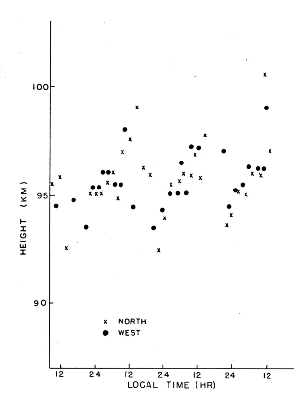
6. Annual number of meteor echoes as a function of height. 59 7. Hourly mean height of meteor echoes as a function of 60

time of day.

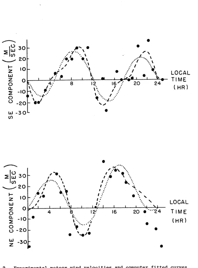
8. Meteor wind components at Sheffield on 14 April 1965.

(a) Northwest component ₆₁

(b) Southwest component 62

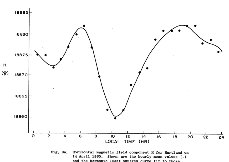
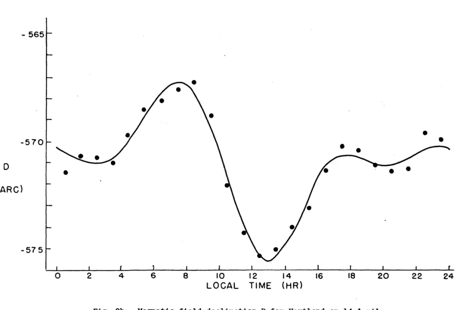
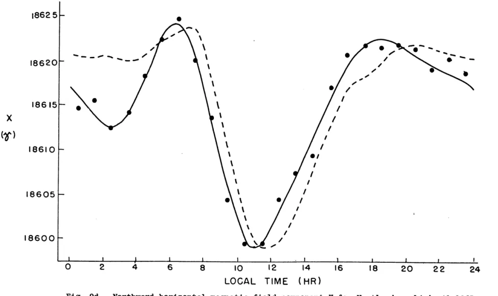
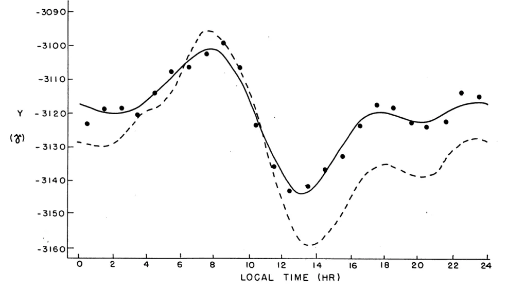
9. Magnetic field measurements at Hartland on 14 April 1965.

(a) Horizontal component 63

(b) Declination 64

(c) Vertical component 65

(d) Northward horizontal component 66

(e) Eastward horizontal component 67

10. Prevailing amplitude of the eastward and northward 114 meteor wind components at Sheffield between August 1964

and August 1965.

11. Harmonic amplitudes of the eastward and northward

meteor wind components at Sheffield between August 1964 and August 1965.

(a) Diurnal amplitude 115

(b) Semidiurnal amplitude 116

(c) 8-hour period amplitude 117

(d) 6-hour period amplitude 118

12. Harmonic phase angles of the eastward and northward meteor wind components at Sheffield between August 1964 and August 1965.

(a) Eastward diurnal phase angle 119

(7)

(c) Eastward semidiurnal phase angle 121 (d) Northward semidiurnal phase angle 122 (e) Eastward 8-hour period phase angle 123 (f) Northward 8-hour period phase angle 124

(g) Eastward 6-hour period phase angle 125 (h) Northward 6-hour period phase angle 126

13. Harmonic phase angle difference between the eastward

and northward meteor wind components at Sheffield between August 1964 and August 1965.

(a) Diurnal phase angle difference 127 (b) Semidiurnal phase angle difference 128 (c) 8-hour period phase angle difference 129 (d) 6-hour period phase angle difference 130 14. Diurnal variation of the height-integrated asymmetri- 145

cal conductivity at the equinoxes.

15. Horizontal height-integrated E-region current density on 14 April 1965.

(a) Southward component 146

(b) Eastward component 147

16. Mean horizontal height-integrated current density.

17. Seasonal mean horizontal dynamo electric field.

18. Mean horizontal total electric field.

19. Mean horizontal residual electric field.

20. Seasonal mean horizontal height-integrated current density.

(a) Southward component 156

21. Seasonal mean horizontal total electric field.

(8)

According to the dynamo theory of the ionosphere as first sug-gested by Stewart (1882) and developed mathematically by Schuster (1908), daily quiet day variations in the earth's magnetic field (Sq) are

attributed to small superimposed magnetic fields of ionospheric currents. These currents are induced by daily periodic ionospheric winds as they move electrically conducting air in a thin layer (90-150 km) across the earth's magnetic field lines. Reviews of the dynamo theory and its mathematical formulation can be found in Chapman and Bartels (1940), Chapman (1963), and Sugiura and Heppner (1966).

These daily periodic ionospheric winds are believed to consist primarily of diurnal and semidiurnal thermal tidal components. These tides originate in source regions above and below the ionosphere, i.e., atomic oxygen absorption in the thermosphere, water vapor absorption in the troposphere, and ozone absorption in the upper stratosphere (Sugiura,

1968). Thus the Sq variations would depend primarily on four ionospheric factors: _{(1) the ionospheric motions as forced by solar heating, (2) the} anisotropic electrical conductivity of the ionospheric medium as a func-tion of the particle density and the intensity of the ionizing solar radiation, (3) the vertical propagation of tidal modes from their source regions, and (4) the main magnetic field strength and orientation with respect to the motion of the ionospheric particles. The prevailing and irregular ionospheric winds also contribute, but to a lesser extent and in an even more complicated manner (Van Sabben, 1962 and Hines, 1963).

In the past the dynamo theory has been used either to derive the magnetic variations from an assumed tidal wind system, (V-,*J formulation),

(9)

or to derive the effective tidal wind system from the observed magnetic variations, (J-->V formulation). In both methods quite arbitrary assump-tions had to be made concerning the space and time variaassump-tions of the mag-netic field and of the ionospheric winds, currents, and conductivities. Thus some reservations must be made concerning the validity of any

derived tidal dynamo current system. In any case published results such as Baker and Martyn (1953) and Kato (1957) show that the inferred ionos-pheric tidal winds are capable of producing quiet day magnetic variations of the same order of magnitude as those observed. In addition, rocket measurements reveal ionospheric currents between 105 and 125 km of the right order of magnitude to produce the Sq variations (Davis, Stolarik, and Heppner, 1965). Unfortunately this is essentially all that is known about the ionospheric current system.

Recently new ionospheric data in the form of meteor wind observa-tions have become available. _{It is therefore the purpose of this study} to utilize this new data to provide some insight into the complex relation-ships between the observed ionospheric periodic winds and the Sq variations in the earth's magnetic field.

(10)

II. DYNAMO THEORY RESEARCH

One of the most successful studies using the J---V formulation of the dynamo theory was made by Maeda (1955). As modified by Kato (1957) his widely referenced results suggested that the tidal winds responsible for the dynamo currents inducing the Sq variations were primarily diurnal rather than semidiurnal, conversely to what has been assumed for many years. However, ionospheric neutral wind observations by meteor trail echo, low frequency radio wave fade drift, and chemiluminescent drift techniques do not directly confirm this. This discrepancy may be due to height-determination inaccuracies and time and areal paucity in these measurements.

For example, the drift wind data (90-130 km) besides being sparse as is the meteor wind data, are not obtainable during daylight hours. Thus tidal wind components can only be inferred, although Hines (1966) developed an empirical method for extracting the diurnal wind components by assuming they reach their maximum amplitude at a prespecified time of

the day.

Further the meteor wind region (80-110 km) only barely overlaps the dynamo current layer. Also the meteor wind data exhibit considerable discrepancies when compared to the derived Sq variation winds,

particular-ly in the ratio of.the amplitudes of the diurnal and semidiurnal compo-nents. Since this may also be due to a change in this ratio near 100 to 110 km, Sugiura (1968) stated that a direct comparison of meteor echo measurements with an effective Sq wind system may not be meaningful.

Moreover the theory of dynamical tidal oscillations in the ionos-phere is not completely known, especially their amplitude attenuation

(11)

and phase propagation with height at different latitudes. Hines (1966) suggested that from simple considerations it was still possible for the diurnal tidal oscillations to be more seriously damped than the semi-diurnal without losing their dominance in the production of the Sq varia-tions.

Also,. if a vertically uniform electric field is applied throughout the dynamo region the direction of the resulting currents changes appreci-ably with height within that region corresponding to anisotropic conducti-vity changes (Hines, 1966). Since the primary tidal winds may also change

by as much as a factor of ten in magnitude, 1800 in direction, and 3600

in phase over the height range of the dynamo region, the consequence of using an integrated current density and assuming vertically constant winds is that the Sq effective wind system represents a net integrated wind system. Hence comparing this wind system to actual wind measurements at any one level by amplitude or phase may not be too conclusive. Ideally it would be better to have global ionospheric wind measurements at several heights, compute the resultant current system, and then compare it with

the equivalent current system derived from the actual Sq magnetic varia-tions (Sugiura, 1968).

Comparing Kato's Sq ionospheric wind system (1957) with Lindzen's model of the thermally driven diurnal tide in the E-region (1967) shows

a significant difference between the latitudinal distribution of the amplitudes of their diurnal components at middle and high latitudes. Note, however, that Kato's computed winds are only those components per-pendicular to the magnetic lines. The part of the wind parallel to the field lines is not computed by his J--V formulation. The difference

(12)

between Kato's and Lindzen's results might be explained by the change in the relative importance in determining the horizontal Sq currents of the dynamo electromotive force versus the electrostatic (polarization) poten-tial field from a small one at low latitudes to a primary one at high

latitudes (Sugiura, 1968). The assumption of vertical constancy of certain parameters in the ionosphere is quite critical and hardly adequate in most cases. It appears that the Sq current systems are also in error the most where the dynamo driving force is the greatest. Wagner (1968) has sug-gested that, since the Sq variations are the result of large area current systems rather than currents above a particular location, then changes in the ionospheric conductivity at high latitudes could affect the Sq varia-tion at lower latitudes but not the ionospheric winds at those locavaria-tions. Further evidence of such errors is apparent in the large discrepancies between various empirical computations of the height-integrated

conduct-ivity at latitudes above 300 latitude, e.g., Fejer (1953) and Maeda and Murata (1968).

Due to the qualified success in verifying the dynamo theory by simple indirect methods, some researchers are now questioning the valid-ity of a simple Sq current system as the connecting link between the ion-ospheric motions and the surface magnetic variations. For example,

Wagner (1968), in investigating the semiannual variation (an equinoctial centered maximum) of the amplitude of the Sq variation, suggested that this variation may not be due to changes in the Sq current system but to a hemispheric asymmetric dynamo or to permanent current systems caused

by nonperiodic ionospheric winds. The latter concept was first discussed by Van Sabben (1962) and later by Maeda and Murata (1968). Wagner

(13)

the solar wind changes due to the varying sun-earth geometry.

Another question was raised by Price (1963) who suggested that the noncyclic change in the Sq variation was due to the subsequent decay of a terrestrial ring current after its intensification during solar magnetic storms. The field of the ring current is nearly uniform at the earth's surface with its direction parallel at all times to the earth's dipole axis. However the resultant current system is not uniform with longitude and is not symmetrical about this axis. Price attributes this to ionos-pheric currents distinct from the ring current but it may be associated with ring current fluctuations or direct solar radiation, i.e., exo-ionos-pheric sources of geomagnetic disturbances.

Price (1964) also states that the prespecified baseline for deter-mining the Sq variations must be an arbitrary one until the ratios of the nighttime and daytime ionospheric currents and conductivities are known.

A necessary assumption in either the J--)V or V-->J dynamo theory formulations is that the horizontal ionospheric currents have zero diver-gence. Price (1968) showed that subsequent derived Sq current systems would correspond to only one part of the ionospheric current system, i.e.,

one of no vertical currents with its horizontal currents giving rise to magnetic fields within the ionospheric current layer. The part neglected then contains both vertical and horizontal currents but with no magnetic fields being produced. Thus the existence of small but widely distributed areas of vertical current flow would change the pattern of the horizontal flow such that there would not be Sq current vortices but a distribution of current sources and sinks at any one level due to these small vertical currents. The divergence of the total current density over the dynamo

(14)

region would be zero and the total vertical flow of nearly the same magni-tude as the total horizontal flow. Consequently the assumption of zero divergence of the horizontal currents becomes more inaccurate at high latitudes.

Therefore, although direct comparison of ionospheric wind data with equivalent Sq current wind systems may not be practical, the basic tenets of the dynamo theory are still valid. There also appears to be definite cause and effect relationships between the ionospheric neutral winds and the observed magnetic field variations.

For example, Appleton (1964) stated that from correlations of the ionospheric electron density indices with the amplitudes of the monthly Sq variation the E-region is the only layer in the ionosphere whose sun-spot cycle variation is identical with that of the Sq variation. There-fore, if ionospheric currents cause the Sq variations, then the E-region

is the only layer in which these currents could flow.

As Hines (1963) suggests, once the mathematical analysis of the dynamo theory is reworked for the dominant diurnal tidal modes, perhaps direct comparisons can be made between the ionospheric wind and the sur-face magnetic data. In the meantime, it is still feasible to examine

the possible relationships between them, particularly if the electric conductivity varies more slowly in time than do the ionospheric winds.

In this vein considerable attention has been focused on the rela-tions between various indices of the E-region ionization and magnetic field indices due primarily to the lack of E-region wind observations and to the necessity for including the effects of conductivity varia-tions (Bibl, 1960 and Heisler and Whitehead, 1964).

(15)

Vestine (1958) speculated that if the changes in the day to day ionospheric wind speeds with the solar cycle are negligible, this infers that the substantial increase in the amplitude of the Sq variation with the solar cycle (Bartels, 1932) is probably a gradual electric conduct-ivity effect, together with a general increase .in wind speed which appears to be gradual only in successive averages taken over many days.

Hence the day to day changes in the Sq current system could arise either from daily changes in the ionospheric circulation or from daily changes in the distribution of the E-region plasma. An assessment of the latter might allow a comparison of ionospheric wind components with mag-netic variations. Then the proposed meteor wind observational program

could be used to assess the effects of large-scale circulation patterns on the geomagnetic field. Newell and Dickinson (1967) and Wulf (1967) have conjectured that changes in the large-scale circulation patterns in the E-region could account for some of the changes in worldwide values of geomagnetic indices. That is, the large-scale motions can affect the dynamo driving force either directly by dynamo action or indirectly by modifying the ionospheric plasma distribution and hence the conductivity of the ionosphere.

Likewise the solar radiation, as the primary source of the large-scale circulation and the periodic motions, can vary the amount and the distribution of ionization. Variation of this ionization with the solar

cycle could be produced by variations induced in either of the above mechanisms (Sprenger and Schminder, 1969).

MWller (1966) has detected week to week changes in the prevailing meteor wind of at least 10 m/sec at Sheffield, U.K. which may be a

(16)

conse-quence of periodicities in the wind system with time scales of several days to a week. He suggested that this indicates the presence of

planet-ary waves in the meteor region. He also comments that from the Sheffield, U.K. and the Kharkov, USSR meteor wind data, there appears to be evidence of a standing wave in the semidiurnal components. However, this may be an over-simplification since the tidal wind variations in conjunction with small ionization variations could produce apparent prevailing wind compo-nents and conversely, tide-like wind compocompo-nents can be established by time-independent pressure gradients acting in conjunction with ionization variations (hines, 1968).

Thus in this study not only will ionospheric periodic wind varia-tions be compared with Sq magnetic variavaria-tions, but also ionospheric pre-vailing wind variations with indices of magnetic activity. Further, simple dynamo theory computations will be performed to determine what seasonal variations exist in ionospheric electromagnetic parameters.

(17)

III. DATA SELECTION AND ACQUISITION A. Ionospheric Wind Data

Radar-echo measurements of the drifts of ionized meteor trails between 80 and 110 km can provide direct information concerning the neutral winds of the ionosphere at these heights. Heretofore similar data were available from rocket vapor trails (Woodrum and Justus, 1968; Robertson et al., 1953- and Manning, 1959). from low frequency radio wave reflections (Sprenger and Schminder, 1967), and from persistent visual meteor trails (Liller and Whipple. 1954). However these methods are necessarily restricted to nighttime hours and thus are not completely suitable for the study of the prevailing and periodic tidal wind compo-nents on a synoptic and continuous basis. Hence the radar-meteor trail technique at present offers the most feasible and economical means for obtaining this goal (Newell and Dickinson, 1967 and Barnes, 1968).

Although the radar-meteor trail technique has gone through consid-erable improvements and sophistications since its inception in the early 1950's (Greenhow and Neufeld, 1955), the basic system remains the same

(Revah and Spizzichino, 1966 and Nowak, 1967).

In particular, at Sheffield University, U.K. (MUller, 1966), a coherent pulse radar system measures the Doppler shift of the ionized trails (under-dense invisible radar echoes) created by minute meteors as they enter the atmosphere and are burned up by the ionosphere in the

80 to 110 km region. Two fixed antennas directed northwest and

south-west respectively are operated alternately at half-hour intervals to obtain wind velocities in two orthogonal directions. Here the wind is assumed to be predominantly horizontal. Using a standard height of 95 km

(18)

for the height of the meteor echoes, the wind velocity in a particular di-rection for one echo is obtained from the range, amplitude, and Doppler shift of the meteor echo as measured by the radar system.

Because of the spread of recorded wind velocities due to the finite width of the aerial polar diagram and due to irregularities in the meteor

region wind structure, Mller stated that it is necessary to obtain a large number of individual meteor echo observations (normally twenty to forty echoes over a period of ten minutes) in order to determine accurately the velocity component in one direction at one particular time. Measurements usually began near or before local midnight and proceeded continuously

for twenty-four hours. The wind velocities V'(t,N) were tabulated for each day's run in terms of direction (NW or SW) where V is the wind velo-city in m/sec, t is the time of the observation in Greenwich Time, and N

is the number of meteor echoes used to determine that particular data

point. Muller then harmonically analyzed the data points in each direction separately and combined the final results to obtain the zonal and merid-ional harmonic components of the meteor region winds at 95 km.

The reliability of the meteor wind data has been confirmed by MUller (1968) who compared the Sheffield meteor wind data directly with simulta-neous low frequency radio wave drift measurements (Sprenger and Schminder, 1968) for twenty-two individual days' runs in the same height region and geographic latitude. He found good agreement in the change of phase and amplitude with height of the semidiurnal wind components as measured

ear-lier by Greenhow and Neufeld (1961) and as predicted by tidal theory and vertical tidal energy flux considerations (Hines, 1968). In addition, Kato and Matsushita (1969) and Kent and Wright (1968) have shown that the

(19)

movement of densely ionized meteor trails from which the meteor wind data is derived actually represents the motion of the neutral gas in the lower E-region.

The Massachusetts Institute of Technology Department of Meteorology has obtained meteor wind data at 85 to 105 km measured at the Edgemount Research Station of Sheffield University in Yorkshire, U.K. from Dr. MUller; it is essentially the same data used in his paper (Mller, 1966).

The experimental data was in the form V' (t,N), as described previously, for the Regular World Days of the International Year of the Quiet Sun

(IQSY) for August 1964 through July 1965. Examination of the actual data revealed that forty of the data days were suitable for an analysis of the day to day variations. The criteria used was that each day's data contain for both the NW and SW direction at least eleven data points covering at least sixteen hours out of the twenty-four hour period of observation. It was this set of forty data days that was used in this study to represent the winds in the E-region.

B. Magnetic Field Data

Since the meteor wind observations were taken at low elevation angles (about 300) with two fixed antennas facing NW and SW respectively, the resultant wind vectors should be considered as representing the mean over a circular area of about 115 km radius centered about 115 km west of Sheffield. In order to relate the meteor wind observations to magnetic

field measurements, a magnetic observatory should be selected within this circle. The nearest observatory thus qualifying is Stoneyhurst, U.K. with Hartland, U.K. the next nearest station to the south. However,

(20)

magnetic observatory. A geographical illustration of this discussion is indicated in Figure 1.

In anticipation of possible relationships concerning the magnetic field orientation and of the need for control stations for solar influ-ences, additional magnetic observatories were selected along Hartland's approximate geomagnetic latitude and longitude.

Data for the Hartland magnetic observatory for the period, August 1964 through July 1965, was obtained from the World Data Center, Boulder, Colorado. It consisted of daily magnetograms of the horizontal component H, the declination D, and the vertical component Z of the geomagnetic field as well as monthly tables of the mean hourly values of H, D, and Z.

Corresponding data in the form of 3 hr K-Indices for all selected magnetic observatories were copied from the Bulletin No. 12 Series of the

International Union of Geodesy and Geophysics, Association of Geomagnetism and Aeronomy. Also the planetary 3 hr K-Index values, Kp, for the forty selected wind data days were obtained from tables in the 1965 and 1966 issues of the Journal of Geophysical Research. The tables entitled "Geo-magnetic and Solar Data" were prepared by J. Virginia Lincoln of the National Bureau of Standards, Boulder, Colorado.

C. Notation and Units

To facilitate the presentation of equations, figures, and tables in this study, the meteor wind and electromagnetic variables were assigned the notation as listed in Table 1. Units of these variables generally are in the rationalized mks system. In addition, the harmonic or periodic components of these variables when applicable were assigned the suffix

(21)

notation as listed in Table 2 to be used in conjunction with the notation of Table 1.

D. Classification of Data

The data sources for this study are listed in Table 3, along with their geomagnetic and geographic locations and the data variables provided

by each source.

The forty meteor wind data days were classified in three ways:

(1) by planetary magnetic activity, (2) by local magnetic activity, and (3) by seasonal characteristics of the ionospheric winds.

In the first case the data days were divided into two groups by their international monthly magnetic classification, i.e., all the data days and undisturbed data days only. In the second case the average daily K-Index at Hartland was used as the daily index of local activity. The results of these two classifications are summarized in Table 4. Note that the month of January 1965 contains no data days, due to an inoperative NW radar antenna at Sheffield.

In the third case the seasonal characteristics used are the weak-ening of the prevailing zonal meteor wind near the equinoxes (Greenhow and Neufeld, 1961) and the advance and recession of the phase of the semidiur-nal drift wind component near the spring and fall equinoxes respectively

(Sprenger and Schminder, 1968). Specifically, Sprenger and Schminder re-ported that the phenomena occurred during the data day period on March 21 and October 15. Thus nine seasonal groupings were formed from the set of forty data days. Their assigned coding and inclusive dates are listed in Table 5. Note that the summer season S contains almost twice as many data

(22)

days as the winter season W. Thus the annual season ANN which contains all the data days is biased towards the summer season. Further the data days were not grouped by months since any monthly statistic based on only four or five random data days was considered unrepresentative. Table

6 contains the number of data days in each of the data day groupings for

a combination of the second and third classifications. Values were given only for those data days groupings used in this study.

(23)

Table 1:

Notation and Units of Meteor Wind and

Electromagnetic Variables used in this Study

VARIABLE

NOTATION

VARIABLE

UNITS

VARIABLE DEFINITION

VAR.

HAR

SW

NW

SE

NE

U

V

H

m/sec

gammas (

)

gammas (1)

Minutes of

Positive Arc

gammas

(1r)

gammas (t

)

degrees(o)

Variable notation

Harmonic Notation

Southwesterly Meteor Wind Component

Northwesterly Meteor Wind Component

Southeasterly Meteor Wind Component

Northeasterly Meteor Wind Component

Westerly Meteor Wind Component

Southerly Meteor Wind Component

Horizontal Component of Magnetic

Field

Downward Vertical Component of

Magnetic Field

Magnetic Field Declination

Southward Component of H

Eastward Component of H

Meteor Wind Velocity Vector

Magnetic Field Vector

Arithmetic Difference Between U

and V

Arithmetic Difference Between Y

and X

Phase Angle

K-Index

X

Y

V

B

U-V

Y-X

0 K

_ _

(24)

Table 1: (cont.)

VARIABLE

NOTATION

VARIABLE DEFINITION

VARIABLE

UNITS

J

Jx Jy DX

DY

ET

ETx

ETy

ED

EDx EDy ER ERx ERy [K] Kxx

Height-integrated Horizontal Current

amperes/km

gammas (1)

gammas ()

volts/km

mho

s

mhos

Height-integrated Horizontal Current

Density

Southward Component of J

Eastward Component of J

Deviation of X magnetic Field

Com-ponent from an Arbitrary Base Value

Deviation of Y magnetic Field

Com-ponent from an Arbitrary Base Value

Total Horizontal Electric Field

Southward Component of ET

Eastward Component of ET

Horizontal Dynamo Electric Field

Southward Component of ED

Eastward Component of ED

Horizontal Residual Electric Field

Southward Component of ER

Eastward Component of ER

Height-integrated Conductivity

Tensor

Southward Symmetrical Component

of K

Eastward Symmetrical Component

of K

Eastward Asymmetrical Component

of K

Kyy

(25)

TABLE 2:

Additional Notation for Meteor Wind

and Magnetic Field Harmonic Components

Used in this Study

*

Harmonic

Notation

PA

DA

SA

TA

QA

DP

SP

TP

QP

Amplitude of

Phase Angle

Harmonic Definition

Prevailing Component (period = o)

Diurnal Component (period = 24 hrs)

Semidiurnal Component (period = 12 hrs)

8-Hour Component (period = 8 hrs)

* 6-Hour Component (period = 6 hrs)

of Diurnal Component (period = 6 hrs)

of Semidiurnal Component (period=1

2

hrs)

of 8-Hour Component (period = 8 hrs)

of 6-Hour Component (period = 6 hrs)

(26)

LIST OF DATA SOURCES FOR THIS STUDY

Variables Observatory

Observed NW, SW H,Z,D,K K K K K K K K K K K K K K K K K

Code Geomagnetic Location

Name Latitude Sheffield, U.K. Hartland, U.K. Stoneyhurst, U.K. Wingst, Belgium L6v8, Sweden Leningrad, USSR Victoria, Can. Agincourt, Can. Eskdalemuir, U.K. Chambion-la-Foret,Fr. Del Ebro,Spain Moca, Fern.Poo.Isles Dourbes, Belg. Wellen, USSR Yakutsk, USSR Tomsk, USSR Sverdlovsk, USSR Kasan, USSR Planetary HA ST WN LO LN VI AG ES CF EB MC DB WE YA TM SV KN

56.6

54.6

56.9

54.5

58.1

56.2

54.3

55.0

58.5

50.4

43.9

5.7

52.0

61.8

51.0

45.9

48.5

49.3 Longitude

76.9

79.0

82.7

94.2

105.8

117.4

292.7

374.0

82.9

83.9

79.7

78.6

87.7

237.1

193.8

159.6

140.7

130.4

Kp Primarily mid-lati

Geographic Location

Latitude

53026'N 51000'N 53051'N 53044'N 59021'N 59057'N 48031'N 43047'N 55019'N 48001'N 40049'N 03021'N 50006'N 66010'N 62001'N 56028'N 56044'N 55050'N

Longitude

1021'W

4029'W

2028'W

9004'E

17050,'E

30042'E

123025'W

79016'W

3012'W

2016'E

0030'E

8

0

.40'E

4036'E

169050'W

129040'E

84056'E

61004'E

48

0

51'E

tude Northern Hemisphere

(27)

Table 4:

Data Classification For This Study

Day Mon Yr 6 12 19 26 9 16 23 7 14 21 28 4 11 18 25 1 16 23 3 10 24 10 17 31 7 14 21 28 5 13 19 26 2 9 23 30 7 14 21 8 8 8 8 9 9 9 10 10 10 10 11 11 11 11 12 12 12 2 2 2 3 3 3 4 4 4 4 5 5 5 5 6 6 6 6 7 7 7 64 65 Data Pts #SW #NW 23 24 17 17 18 19 16 19 13 17 17 21 17 20* 15 20 18 19 15* 17 18 15 16 11 16 16 15 16 16 13 13 18 14 15 13 14 14 17 13 24 22 18 17 18 19 17 19 13 18 12 22 17 20* 17 19 19 19 15* 14 18 15 16 12 16 16 16 17 12 13 14 17 13 16 14 12 14 15 13 28 7 14 14 Total 659 652 Average 16.5 16.3 Hartland K Data K 3311 4233 0012 3321 2323 1211 2232 4322 3322 3222 2111 0201 0121 0213 0000 2212 3212 1120 1003 2223 3222 2001 0110 1210 3301 2101 1000 2110 4543 0000 0111 1111 1121 3322 1001 2222 2221 2110 2110 3332 1002 1.38 3342 3.00 2213 1.38 3223 2.38 3343 2.88 3333 2.12 1012 1.62 1134 2.50 1002 1.62 3342 2.62 2132 1.62 2113 1.25 1112 1.12 2100 1.12 0120 0.38 2222 1.88 5122 2.25 1102 1.00 3212 1.50 2232 2.25 2123 2.12 1000 0.50 2321 1.25 0001 0.62 2212 1.75 2102 1.12 1210 0.62 1110 0.88 2433 3.50 1211 0.62 1000 0.50 0222 1.25 2231 1.62 3332 2.62 1110 0.62 3334 2.62 1223 1.88 1312 1.38 1110 0.88 3333 2.88 Int'l Code N D N N N N N N N D q N N N

Q

N D N N N N

Q

q N N N Q

Q

D

Q

Q N N D q D N q q D 6Q 7D 5q 22N K10.5 K51.0 KS1.5 K-2.0 K52.5 x x x x x x x x x x x x x x x x x x x x x x x x x x x x x x x x x x x x x x x x x x x 3 9 20 27 34 1.63

(*=24 hr period of observation began at 1200 LT; Q=One of 5 most quiet days of month; D=Qne of 5 most disturbed days of month; q=One of 10 most quiet days of month; N=Normal day; K=Mean daily Hartland 3hr K-Index)

(28)

SEASON SUMMER

WINTER

Table 5: Coding and Definition of Seasons for this Study

CODE INCLUSIVE DATES

EQUINOX NONEQUINOX SUMMER SOLSTICE WINTER SOLSTICE SPRING EQUINOX FALL EQUINOX ANNUAL NE

SS

WS

SE FE ANN

(Aug 1

-

Oct 14) 1964 and

(Mar 22

-

Jul 31) 1965

(Oct 15, 1964 - Mar 21, 1965)

(Aug 1 - Nov 5) 1964 and

(Feb 11

-

May 5) 1965

(Nov

(May

6, 1964 - Feb 10, 1965)

6, 1965 - Aug 1, 1965)

(May 6 - Aug 1) 1965

(Nov 6, 1964 - Feb 10, 1965)

(Feb 11 - May 5) 1965

(Aug 1 - Nov 5) 1964

(Aug 1, 1964 - July 31, 1965)

Table 6: Seasonal Classification of Data Days

for this Study

MAGNETIC CRITERIA S W E NE SS WS SE FE ANN All (R<3.5) K<2.5 K<2.0

K<1.5

K<1.0 K>1.0

K>1.

5

26

14

20

11

9

11

40

21

13

17

10

12

15.

-- --

--

34 --

--

27

-- -- -- -- -- --

20

-- -- -- -- -- -- -- -- 9

20

11

-- -- -- -- -- --

31

-- -- -- -- -- -- -- -- 20

(29)

0 ESKDALEMUIR

(

STON SHE FFIELD

0

HARTLAND 5 4 3 2 I 0

LONGITUDE

(Ow)

Fig. 1. Geographical location of principal data sources. Points (1), (2),

and (3) represent the meteor echo location for Sheffield's NW meteor radar antenna, the meteor echo location for Sheffield's SW meteor radar antenna, and the epicenter for an observed meteor wind vector at Sheffield, respectively for meteor echoes observed at 95 km using a 270 antenna elevation angle.

56-

55-

54-z o LJ 53 52 -511

(30)

IV. DATA PROCESSING

From tidal and dynamo theory considerations, the following method was chosen to relate the meteor wind observations to the magnetic field measurements. Each data day's set of meteor wind and magnetic field data were to be harmonically analyzed for their prevailing and periodic compo-nents. These components then were to be linearly correlated to establish whether or not direct relationships exist between the two types of data.

A. Meteor Wind Data

Although magnetic field measurements were available for each hour of each data day, this was not so for the meteor wind observations. Avail-able were only twelve to twenty-five individual data points scattered at somewhat irregular intervals throughout each data day. To obtain meteor wind data corresponding to the magnetic field data, hourly meteor wind values necessarily had to be generated from the given meteor wind data. The most common method of performing this generation is by a least squared harmonic analysis technique. In the following section this method as used

by MUller (1966) will be discussed. Then the method selected and used for

this study will be outlined in detail.

1. Discussion of methods of harmonic analysis

The method of harmonic analysis which MUller (1966) used is as follows. A typical data day's set of experimental data points is shown

in Figure 2, where the data points represent the horizontal meteor wind velocities for each antenna direction. Superimposed are the results of MUller's harmonic analysis.

(31)

draw by hand a smooth curve across the experimental data points and then make a Fourier analysis of the curve to resolve the prevailing and periodic

components. _{He felt that a considerable bias might be introduced by this} method, particularly if the number of meteor echoes contributing to a given data point was small. _{Therefore to obtain a more objective wind} pattern, he computed a least squares curve fit to the experimental data points, using a constant and four harmonic terms and giving weight to each point according to the number of meteor echoes used in determining that point.

Specifically, a curve was required to fit an equation of the form

V(t)=A,,

+{AN;

c s

t) + At)

(4.1)

where V is the harmonically approximated wind velocity, t is the time in hours from local midnight, A is a constant, and the Ai's are harmonic amplitudes. _{The experimental data points are of the form V'(t,N) where t} is as defined above and N is the number of meteor echoes used in determin-ing the data point wind velocity V'. It was now required to minimize the function

Y=

zIN[V(t)-V(tNZ}

(4.2)

where the summation _{here and throughout the remainder of this} sec-tion is over the data day's set of experimental points V'(t,N). This was done by forming the partial derivatives

(32)

aY

Y

3Y

a A, "A'

and equating them to zero, obtaining nine simultaneous equations with nine unknowns.

The set of nine simultaneous equations are of the form

N{Ao+

[Azi_.

coS(Z) +A,,s.,(

2)]

=

z

N V'(t,

N)

t)

(4.3)

where j =

N

A

,..., 4

+

[A

os

,,,cos(N

-+A)

t)

I

N

V'(t,

N)

cos(

t)

(4.4)

where k = 1,...,4

These equations after substitution of the experimental meteor wind

data were then solved for A, A1,. . . . A8. Reordering the equations yielded a symmetric coefficient matrix which is easily solved by computer.

(33)

After computing the velocity components for each data day for the NW and SW data points separately in the form of equation (4.1) the trans-formation was made to the final form

V(t) V +

_I

(slN

t-

(.6)

by the following equations

VO

A

0 (4.7)

Vk (A

+ (A

J

(4.8)

Sarcta4[-A

i/A]

(4.9)

for 1 = 1,..., 4 and where Vo is the prevailing wind component, i is the order of the harmonic term, Vi is the amplitude of the harmonic wind compo-nent of period 24/1 hours, t is the time in hours after local midnight, and 0i 2 _{is the phase expressed in time of day when the amplitude V}_i

reaches its maximum value in the direction of the particular wind component being harmonically analyzed. The phase angle

01

ranges from - ~? to + 7T.

These amplitudes and phase angles were then compounded to give the zonal and meridional wind components in the form of equation (4.6).

Since only four or five days of data were available for each month, Mller obtained monthly averages by grouping all the month's data together and using the above method. For seasonal averages he first obtained sea-sonal averages of the experimental data points for each hour of the day

(34)

and then fitted a curve to these hourly averages in the same manner.

MUller (1966) also discussed the error in determining the meteor winds by this method. He computed the theoretical error taking into

account the following effects: (1) the finite width of the antenna polar

0

diagram (a beam width of approximately 48 between half-power points), (2) the error in phase measurement (Doppler shift), (3) the departure of the true meteor height from the assumed standard height of 95 km, and

(4) the error in radar range measurement. He presented the results in a figure plotting the 95% confidence limits of the expected error as a func-tion of the number of meteors contributing to the wind velocity for a single data point. He also plotted on the same figure the actual error for a sample data point. This figure is reproduced here in Figure 3. He then stated that for points where less than fifteen echoes have been used, the error is larger than the theoretical error due to the presence of a vertical wind shear and to short term fluctuations in the wind (apparently due to gravity waves with periods generally of 30 to 270 minutes). The latter, he stated, would have little effect on results obtained from a series of meteor echoes observed over periods of less than ten minutes.

Overall, Miller's procedure seems to be quite logical and correct. However, considering such factors as the annual and diurnal variability in the number of meteor echoes observed, the diurnal variability in the height of maximum occurrence of meteor echoes, the actual error in wind velocity from the observation of only one meteor echo, and the height variability of the prevailing and tidal wind components in amplitude and

in phase, MUller's method appears to be somewhat questionable. It repre-sents a significant departure from that used by other meteor wind researchers

(35)

such as Greenhow and Neufeld (1961), Nowak (1967), Elford (1959), Roper (1966), and Revah and Spizzichino (1966). They all obtained meteor wind

components by a harmonic analysis of hourly averaged winds without weight-ing them by the number of meteor echoes used.

Evidence of a possible discrepancy is the lack of any phase differ-ence between the eastward and northward diurnal wind components in Muller's results (1966) whereas tidal theory predicts a phase difference of 90 . Another indication is shown in Muller's results for a sample data day

(Reference Figure 2). His harmonic curves between 2000 and 0200 hours local time appear to depart significantly from the data points.

To investigate this questionableness, first considered was the diurnal variability of the number of meteor echoes observed. An examina-tion of the hourly number of meteor echoes observed over the period of the Sheffield data revealed that the hourly rate between midnight and noon was two to five times as great as the rate between noon and midnight. An example of typical hourly rates of observed meteor echoes is given in Figure 4 reproduced from Nowak (1967). Hence, in weighting data points

by the number of meteor echoes determining them, the data points although

equal in number before and after noon were weighted considerably more before noon than after noon. Therefore, unless the data points before noon are much more accurate than those after noon, the weighting criteria could be an improper one to use, as is indicated in Figure 2.

The second factor was the diurnal variability of the height of meteor echoes. For his data MUller assumed a standard height of 95 km for

(36)

radar transmitter wavelength as shown in Figure 5 (Nowak, 1967). The ver-tical profile of meteor echoes approximates a Gaussian curve about this standard height, as shown in Figure 6 (Roper, 1966). As shown by the hourly rates of meteor echoes in Figure 4 and by the hourly mean height of meteor echoes in Figure 7 (Nowak, 1967), the height of a meteor echo can vary by as much as five kilometers from a given standard meteor echo height. Hence, the assumption of the data points before noon being more accurate would be enhanced, since the meteor echoes before noon are nearer to the assumed standard height. In turn, this further solidifies the standard height assumption.

The third factor was the actual error in a wind velocity determined from only one meteor echo. An estimate of the standard deviation of a measured wind velocity can be obtained using MUller's error curve values for N = 1 in Figure 3. Since his 95% confidence limits represent approx-imately two standard deviations from the mean and since Mller's curves approximate the function (N)-_{I, the standard deviation of the wind} velo-city based on one meteor echo was estimated to be not greater than 10% of the actual wind velocity. Considering an extreme wind velocity of 80 m/sec, its standard deviation then would be at most 8 m/sec. In MGller's tabu-lated results (1966), the fourth and fifth harmonic terms were at least as large as this. Hence, by neglecting the higher order harmonic terms in the harmonic analysis, an error is made that is probably at least as large as the error eliminated by weighting each data point by the number of meteor echoes determining it.

The fourth factor was the height variability of the prevailing and tidal meteor wind components. From previously referenced meteor wind

(37)

research and from theoretical tidal considerations (Hines, 1968, Lindzen, 1968, Butler and Small, 1963, and Siebert, 1961) this variability has characteristics as follows. The prevailing wind tends to increase with height, about 0.5 to 3 m/sec/km, at least up to 105 km. The diurnal tidal amplitude increases slightly with height.but with a decreasing ver-tical energy flux, approximately by a factor of 1.2 to 2 over the height range 80 to 100 km. The diurnal tidal phase advances with height at about 10 to 200/km. The semidiurnal tidal amplitude apparently increases with height inversely as the square root of the ambient density in order to maintain a constant vertical energy flux, approximately by a factor of ten over the meteor echo height range. Its phase also advances with height but at only about 4 to 8 /km. Hence the assumption of the standard echo height would affect the diurnal component more than the semidiurnal component. Since the diurnal component often has a comparatively large amplitude, it is even more necessary to solidify the standard height

assumption, particularly if the diurnal meteor echo height range is large.

The last factor considered concerns the consequences of the first factor discussed, i.e., the harmonic analysis for prevailing and periodic components of data extending only over a portion of the longest period of the components analyzed. Since MUller weighted the data over the first half of the day much more than the second half of the day, he essentially analyzed for harmonic components with periods up to twenty-four hours using only twelve hours of data. As discussed previously for the drift wind data (Hines, 1966), this requires that the phase angle of the diurnal component be prespecified. This perhaps is the reason for the lack of any phase difference between Mdller's diurnal tidal components

(38)

while tidal theory predicts a 90 phase difference. In other words, his diurnal phase angles were predetermined to some extent by the times of day when data points were determined from a large number of meteor echoes. Further an inaccurate diurnal component will affect the accurately com-puted prevailing and semidiurnal such that they would be valid only in a qualified sense (Sprenger and Schminder, 1967). This fact is continu-ously emphasized by rocket trail and drift wind researchers. However, it could be argued that since the diurnal component is usually smaller than the semi-diurnal component, its effect on the other components would also be small. Based on sample calculations of the Sheffield data this appeared to be true using both weighted and unweighted data points. Because of its premise, this argument is rather weak.

Based on these considerations, the following conclusions were made concerning MUller's weighting procedure:

(1) Using this procedure could produce results significantly different from those using an unweighted procedure by favoring measurements when the number of meteor echoes is large.

(2) This procedure, although placing emphasis on more ac-curate data points and solidifying the standard height assumption, can introduce a significant spurious diur-nal component into the results, e.g., predetermined diurnal phase angles.

(3) Data points which are based on individual or only a few meteor echoes are in error by no more than the errors introduced by neglecting higher order harmonic

(39)

terms and by reducing the time range of the data from twenty-four hours to about twelve hours.

Therefore, for this study it was not necessary and probably in-advisable to use M'dller's weighting procudure in performing harmonic analyses of the Sheffield meteor wind data. However, if his method was to be used it might be appropriate to assume a maximum allowable value for the number of meteor echoes contributing to one data point such as N = 5, i.e., consider all values of N greater than five as equal to five. This would probably incorporate the advantages of MUller's procedure without introducing the errors discussed above.

2. Harmonic analysis method used in present study

Based on the conclusions of the preceding section, the following procedure was developed for the meteor wind harmonic analysis used in this study.

The meteor wind data points for each of the forty data days for each antenna direction (NW and SW) were substituted into the nine simul-taneous equations (4.3), (4.4), and (4.5) with N set equal to one for

each data point. In this way each data point is counted equally, regard-less of how many meteor echoes were used in its computation. This set of

simultaneous equations were solved for the coefficients, A , A1,..., A8

(Hildebrand, 1956) and resolved into the form of equation (4.6) for each antenna direction on each data day. Thus the NW and SW meteor wind com-ponents are obtained as

NW(t)=NW

o+ N

SINt-

(410)

(40)

S/(t)=

S

Wo+

S WA

SIN(

t-0

(4.11) However, the geographical locations at which equations (4.10) and (4.11i) are valid are approximately 230 km apart (Reference Figure 1). Additionally, wind velocity components are usually expressed in terms of eastward and northward components. To resolve both of these problems, equations (4.10) and (4.11) were compounded to give equations in the form of equation (4.6) for the eastward and northward wind components (U and V) as

U(t) U h.hSIN

t8A

(4,12)

V(t)h

V

*VS

(4.13)

First, by basic trigonometry

U(t) = [SW(t) + NW(t)] sin 450 (4.14) V(t) = [SW(t) - NW(t)] sin 450 (4.15) Then assuming each harmonic component satisfies equations (4.14) and (4.15) gives

U = W + NW sin 450 (4.16)

V =

[

- NW] sin 450 (4.17)

(41)

for i = l .... , 4 (4.18)

SIN

SW

s-0k

SIN

45

for i = 1,....,4 (4.19)

Solving equations (4.18) and (4.19) simultaneously for ,

V

, and "A in terms of the known parameters (NWi, SWi, 0i' and 0i) the solutions are

S1=ISWN

+NsW,sIN$+N

s

i+

(s

cosk

+NW

cos

(4.20)

=

arctai

S

i

IN[(S+s

N

S

N

/

_,(cos+N

cos)

(4.21)

M=

(SWIala

SIlN

8 -N

+

(Scos

-NWC OS

j

(4.22)

i=

arctan(SWslN;-NW

_{sIN /(Sjos5r-N/cos0)]}

(4.23)

Thus by substituting equations (4.16), (4.17), and (4.20-4.23) into equations (4.12) and (4.13) the transformation from meteor wind data points in terms of northwesterly and southwesterly components to eastward and northward harmonic components was accomplished.

(42)

By the above procedure the eastward and northward meteor wind pre-vailing components and harmonic amplitudes with their respective phase angles were computed for each of the forty data days.

Also required for later computations was the magnitude of the

total meteor wind velocity

V(t)

.

The following formula was used

V(t)

=

U(t)

+

[

2 (4.24)

where values of U(t) are obtained from equations (4.12) and (4.13).

A further computation was suggested in Newell and Dickinson (1967), i.e., the meteor wind prevailing and tidal northward momentum transports. The northward momentum transport by the prevailing meteor wind is given by U .V . For each tidal component the transport is given by the factor

o

j.Ul.V.cos( i--i. . The mean transports were computed for nine dif-ferent seasons using all the data days available in each particular sea-son.

3. Time averaging of harmonically analyzed values

One additional process was applied to the meteor wind data. To put the meteor wind data into the same form as the magnetic field data, i.e., mean hourly values for each data day, required that the harmonic approximation to the original meteor wind data be time averaged over a period of one hour.

A centered time averaging integration formula was applied to the meteor wind harmonic approximations which were in the form of equation

(43)

T-At

T-At;

T-At

(4.25)

where T is the central time, At is one half the interval of the integra-tion, and V is a particular meteor wind velocity component.

The solution to the integration is of the form -4

V(t=T)-

V-

SIN

At) V SINQ

T-(4.26) For this study At was chosen as 0.5 hours and T as X.5 hours where the X's are integers running from 0 to 23. Thus values of U(T) and V(T) were obtained for each hour of each data day.

Examination of the time averaging formula (4.26) revealed that it has the same form as equation (4.6) except that the harmonic terms of order 1 and greater are multiplied by the factor 24 sin 27it

2iAt sn 24 for i = 1,2,3,4. For At = _{0.5 hours, the factor equals 0.996 for}_{i =} _1,

0.987 for i = 2, 0.954 for i = 3, and 0.826 for i = 4. Taking theoretic-al extreme vtheoretic-alues of Vi and 01, i.e., Vi = 100/i m/sec and all Oi's

identical, the value of V(t=T) differs from V(t=T) by at most 5 m/sec when five harmonic terms are used. Thus it is within the error limits of the initial harmonic approximation as discussed previously to use the hourly averaged values V(t=T) in place of the actual values of V(t=T). Then the hourly averaged values can be plotted as points at the times t=T and a smooth curve drawn through these points for a particular com-ponent on each individual data day.

(44)

To compare the final results, i.e., U(T) and V(T), with the original meteor wind data required that NW(T) and SW(T) be computed. The formulas used are

NW(T) = U(T) - V(T)J sin 45 (4.27)

SW(T) U(T) + V(T) sin 450 (4.28)

The comparison for a sample data day is shown in Figures 8a and

8b. The harmonic approximation is quite good for the SW component and rather poor for the NW component. Further comparisons on other data days showed that this day's NW component's approximation represents an extreme case and that, in general, the generation of hourly wind data by harmonic approximation is a practical method. The primary reason for this seems to be the dominance of the semidiurnal tidal component at 95 km at high middle latitudes.

B. Magnetic Field Data

1. Harmonic analysis

The harmonic analysis method outlined in Section IV.A.2. was also applied to the magnetic field data from Hartland, i.e., the mean hourly values of H, D, and Z for each data day. These values were denoted as H'(T), D'(T), and Z'(T) respectively. Since these were originally aver-aged about the half hour, the valid time of the values was chosen as that

time. Thus the magnetic field declination D and the horizontal and ver-tical components of the magnetic field (H and Z) for Hartland on each data day were approximated in the form of equation (4.6) as