Applications of two dimensional multiscale stochastic models Mark R. Luettgen.

(1)

January, 1992

LIDS-

P 2088

Research Supported By:

AFOSR grant F49620-92-J-0002 NSF grant MIP-9015281 NSF grant INR-9002393 ONR grant N00014-91-J- 1004

Applications of Two Dimensional Multiscale Stochastic Models

(2)

LIDS-P-2088

Applications of Two Dimensional Multiscale Stochastic Models

Mark R. Luettgen' January 29, 1992 Department of EECS, MIT

Room 35-439

Cambridge, MA 02139, USA Telephone: (617) 253-6172 e-mail: luettgen@athena.mit.edu

Abstract

This paper discusses a class of multiscale state space models and their applications. The models are defined on quadtrees and are Markov in scale. Associated with the

models is a smoothing algorithm which calculates the least squares estimate of a process given noisy data over some portion of the corresponding quadtree. This work applies these multiscale models and smoothing algorithms to some typical image processing problems, compares the results to standard approaches, and suggests directions for further research. The problems considered are optical flow and image reconstruction.

1 Introduction

Recently a new class of multiscale stochastic models was introduced [4, 5] along with asso-ciated smoothing algorithms. The models were originally motivated by the wavelet trans-form synthesis equation, and have been shown to approximate Gauss-Markov and 1/f type processes well. The models and algorithms were applied to a number of one-dimensional smoothing problems; the results were promising and motivate application of the ideas in two dimensions. In this paper we describe work in this area on optical flow, surface recon-struction and sensor fusion. The results are compared to standard approaches and are used to suggest directions for further research.

Consider a stochastic process defined on a quadtree (see Figure 1) with the following model:

x(t) = Axz(t) + Bw(t) (1)

where x(t) C RZn, w(t) C Tlm. Associated with each node x(t) is a parent node x(7t) and four descendent nodes, except for the top (root) node of the tree which has no parent. It is assumed that the root node is a Gaussian random variable with variance P, an(l that the driving noise is normally disributed and white: E{w(t)zw(s)'} = O if t 4 s and E{w(t)w(s)'} - Q(m) if t = s. Motivated by the results of Wornell [19, 20], we set Q(m) =- 4-4Lm where it is a constant and m is the scale (the root node is scale zero, the next level of four nodes is scale one, etc.) For instance, in a scalar process if it - 1, B = b and Po = b2 then at each level the same total noise energy (sum of the variances over the scale) is added to the tree process.

(4)

Figure 1: Quadtree structure

Sample paths from several processes are illustrated in Figures 2 to 5. The processes are shown as mesh plots to better illustrate the changes induced by choosing different model parameters. The parameters used to generate them are in Table 1. In all four processes,

figure A l

2 1 1

3 0.5 1

4 1 2

5 0.5 2

Table 1: Tree process sample path parameters

B = Po = 1.

Associated with each node of the tree there may be noisy measurements:

z(t) = Cx(t) + n(t) (2)

where z(t) E 1RP, n(t) C 7RP and n(t) is white Gaussian noise: E{n(t)n(s)'} = 0 if t $ s and

E{n(t)n(s)'} = R if t = s. In [4, 5] iterative and recursive algorithms are developed for the

estimation of the state process x(t) given the measurements z(t) at one or more scales. The algorithms calculate smoothed estimates, that is, the linear least squares estimate (LLSE) of the process at each node given measurement data from all nodes. The algorithm is actually somewhat more general than this statement suggests: it actually calculates the LLSE of the process given any subset of nodes on one or more scales. Thus the model and algorithms

(5)

(6)

Figure 3: Sample path: A = 0.5, B = 1, I = 1

(7)

Figure 5: Sample path: A = 0.5, B = 1, i = 2

provide a natural framework for approaching problems of sensor fusion and situations where only sparse measurement data is available.

2 Optical Flow

The apparent motion of brightness patterns in an image sequence is referred to as the optical flow. The classical approach to calculating the optical flow utilizes the Horn and Schunk [11] brightness constraint equation, which captures a relationship between the temporal and spatial brightness variations:

d 0

0 = dE(, y, t) = E(, y, t) + VE(x, y, t)- v(x, y, t) (3)

where E(x, y, t) is the image intensity as a function of time and space,

VE(x,y,t) = [ xE(x,y,t) ayE(x,y,t)] (4)

(x, y, t)

=

[

y(xy,t)

(5)

and v(x, y, t) is the optical flow vector field. The brightness constraint equation says that the total time derivative of image intensity is zero - that is, changes in intensity are do only to motion of the scene. This equation constrains only the component of the flow field in

(8)

the direction of the gradient, and thus is not enough to compute a unique solution to the optical flow problem. To obtain a unique solution some additional constraints are required. Horn and Schunk proposed a smoothness constraint on the flow field which transforms the optical flow problem into the following minimization problem: (for notational simplicity the arguments of the variables are suppressed):

argmin ₍₆₎

= v

J

R

(dE)a

+

IlVv ll2

+

Il.w "l

(6)

The constant R allows one to tradeoff between relative importance in the cost function of the smoothing and brightness constraint terms.

In actual applications, the minimization problem above is discretized. One way to do

this is to estimate the temporal gradient as the difference of two frames, °E(X, y, t) t

E(x, y, t + 1) - E(x, y, t) and to estimate the spatial gradient based on a convolution of E(x, y, t) with a smoothing kernal and a directional derivative kernal. This formulation

provides the optical flow at time t given frames at times t and t + 1. Alternatively, we could interchange the roles of the two images, and compute the optical flow at time t + 1. This is in fact what is often done in motion compensated image coding applications. Since we will use a coding metric as one means of evaluating the quality of the tree based optical flow estimates, this is the formulation we use below.

2.1 Optical flow estimation using tree models

The optical flow problem formulation above can be interpreted in an estimation context. Specifically, define:

z = tE(, y, t) (7)

C = VE (8)

Now consider problem of estimating the flow field from noisy gradient measurements, under the assumption that the flow field is a sample path of a two dimensional Brownian motion:

z= C v + n (9)

with:

n Af/(O, R) (10)

Vv, = VB2(x,y) (11)

Vvy = VBy(x,y) (12)

where B, and By are two-dimensional brownian motion processes with covariance:

E{B(xi,

yi),

B(X2, Y2)} = (x + y2) + (x2 + y22) - ((x1 - x2)2 + (Y1 - y2)2) (13)

It is shown in [15] that the solutions to the Horn and Schunk formulation and the estimation formulation are the same. The estimation formulation allows us to interpret the smoothness constraint as a prior model for the velocity field. This prior model is fractal in the sense

(9)

Figure 6: Fractal velocity field

that the penalty depends only on the gradient of the field, not the magnitude. Thus, the three (one-dimensional) fields shown in Figure 6 are equally likely prior processes. This suggests that the Brownian motion term could be replaced with a term corresponding to a tree process, which also exhibits statistical self similarity and has been shown to be a good approximation to fractal processes [5, 19, 20]. With the Brownian motion replaced with a tree process prior model, we have a problem exactly as formulated in [5] in which there are noisy measurements of a tree process and a smoothed estimate is desired. One advantage of this formulation is in the computational efficiency of the tree model estimation procedures.

A particular set of parameters for the tree model need to be chosen for the smoothing algorithm. A reasonable assumption is that the x and y components of the velocity are uncorrelated. Thus, we choose A = aI and B = bI. The matrix C comes directly from the spatial gradient calculations. Except for the first two examples, the spatial gradient was computed by smoothing with a Gaussian lowpass filter of support 3 x 3 and variance 1 followed by a central difference approximation to the first derivative. The first two examples utilize noiseless artificial images, thus the prior smoothing is not done.

The prior covariance is set as Po = 100.I to avoid setting an apriori mean for the velocity field. Equivalently, we could find the maximum likelihood estimate (maximization of the conditional measurement density, given the flow field). The measurement noise variance is

set as r = max(rllIC112, r2) where rl and r2 are constants The idea here is to penalize large

gradients since these are likely points of occlusion where the brightness constraint equation

will not hold [16]. Unless noted otherwise, the constants were set as rl = 1, r2 = 10. Finally,

(10)

In summary, the constants a, b and p are parameters which can be varied to control the degree and type of regularization imposed on the velocity field. Ideally, we would use some system identification procedure to determine the parameters from image to image, or even adaptively within an image. But this is still an open problem, so as a first approximation the parameters are set in an ad-hoc way in the examples below.

Finally, we consider methods for evaluating the quality of the flow field estimates. In general, these depend on context: will the optical flow be used for image interpretation, motion compensated coding, three dimensional motion analysis, or some other application? In this paper, two metrics will be computed and the reconstructed fields will be presented so that the flow estimates can be evaluated in a variety of ways. The first metric is motivated by coding applications. It is the mean square reconstruction error of a frame at time t + 1 given the flow field at time t + 1 and the frame at time t. The frame at time t + 1 is reconstructed using a bilinear interpolation of the frame at time t. Specifically, a point in the grid at time t + 1 is projected back to time t using the estimated optical flow. This point in general does not lie on the image grid at time t and thus must be estimated. One way to do this is by interpolation using the four nearest neighbors as shown in Figure 7.

The bilinear interpolation used is as follows:

tE(t

+ 1,, y) = (t, + (t + 1),y + v(t + 1))

= E(t,

X',y')

= co + c₁Ax + c₂Ay + C3aXAy (14)

where:

Co = E(t, ,y)

cl = E(t, , y)- E(t, ,y)

c2 = E(t,

,

y)- E(t, , )

c3 = E(t, , ) + E(t,, y) - E(t, , y) - E(t, x,)

Ax = x'

-ay

= y'-Y

and E(t, x, y) denotes an estimate of the intensity at time t and location (x, y). Of course, one could also compute the flow field at time t, project this forward to time t + 1 and then interpolate. This is more difficult since there will be one grid point interpolated from four non-grid points. Note also that this metric is computable even if the actual flow field is not known. In addition to this metric, the mean square error in the flow field components is also computed in the examples below. Note that the two metrics will in general provide conflicting results - lower mean square error in the flow field estimates does not necessarily indicate lower error in the image reconstruction. For instance, in regions where the image intensity is constant, there may be large flow errors with no image reconstruction error. Also, smooth flow fields are more visually pleasing than non-smooth fields, yet the non-smooth fields generated by pel-recursive techniques often provide much lower image reconstruction error in coding applications [2, 18].

(11)

Ax

(xI ,y')

Ay

* (%,y)

*

<xtu

Figure 7: A projected point and it's four nearest neighbors

2.2 Examples

The first example is of a simple translation of an image. The first 64 x 64 image is a Gaussian surface:

E(x,y,ti) = k exp(--z'Z-lz) (15)

z

=

- 30

(16)

Z

1000

500 (17)

[ 000 50]

and the second frame is equal to the first, translated by .1 pixels up and .1 pixels to the left. The constant k is set so that the image has a maximum value of 127.

The C matrix is computed using a central difference method in both directions and the temporal gradient comes from differencing the two images. No noise was added; the point of these initial examples is to provide insight into the nature of the regularization imposed by the tree model. The image and computed gradient are shown in Figures 8 and 9.

Figures 10 and 11 illustrate the computed optical flow for different values of the pa-rameters and Table 2 summarizes the results of four experiments. In this example the regularization is required in the upper right and lower left portions of the image plane where the image gradient is not in the direction of the optical flow. In Figure 10 the regu-larization imposed by the tree model is not strong enough; since a = 0.5, there is significant decorrelation from scale to scale and the prior model does not induce a highly structured

(12)

Figure 8: First frame of translation sequence

flow. In Figure 11, the scale to scale correlation is retained and the resulting estimate is much better.

Test a (A = aI) b (B =

bI)

p RMS Flow error (x, y) RMS reconstruction error

1 0.5 10 0.35 0.03, 0.03 0.032

2 1 10 0.7 0.00075, 0.00072 0.041

3 1 10 0.35 0.0018, 0.0015 0.041

4 1 20 0.35 0.0043, 0.0037 0.040

Table 2: Translation example parameters and performance criteria

The second example used a sequence of Gaussian images modulated by a spatial sinewave. Specifically,

E(x,y, tl) = k sin(atan(x, y)) exp(-1ZZ-'z)

(18)

(19) where z, Z and k are as in the previous example and atan(x, y) is a 27r arctangent. The modulation by the spatial sinewave provides additional gradient information. The second frame is equal to the first, rotated by 1 degree. The spatial and temporal gradients are computed as in the previous example. The first frame and image gradient are illustrated in Figures 12 and 13. In this case the regularization is required in the lower right and upper left hand corners.

(13)

/ I I (//////// I I ////'

//.''// I I / t I\,.~. /f

;/// //I/ I / ,////////,,...

;/,,' _cC)I---~~~-/////-~Y" //tr/ " /J///I1 I f I t ' / 1/ /////7 .t I t ~ ' / , .. I ,I .7 ,,.,.-.. .

-,,/~r~,,,/ ,,'z/1 ,,,,/// ///fI ll/l/ fi/ lit l! ttl /ttt',~ ~'~ x,,x.x.Xx,

/7/////////// / / I I t

,,///////////\/ / /\I \\

~\

\ \\,.

Figure 9: Spatial gradient of previous image

..'... \ \ \ \ \ \ \ \ ,, \\ \\N ...- N\ \ \ \ \ \ .. ...~, \ ,\\\\\ \ ' N N N N N ... , ,\ _-N'--\\\ \ \N '\ \ \ \ N

~~~-....

,,,, \ , ' \ \ \ \\\N ...., ,, ~, ~\\ ~\\ \ \ \ \'t\

~~~\

\

Figure 10: Translation example flow field: a =0.5, b =10, p 0.35

1i 'NNNNN\\\\~~~zN A A A \ A A A I A A A A A N N \\\\\~\\\\\

(14)

\ \ \ \ \ N N \ .N \ N \ \\\\ \ \ \ \ \ \ \ \ \ \ NNNN \\\\\\\\\\\,'\. NN NNN\\ \.\... \N\\

\\\.\ \\\ \ \ \\\.\.N\\\\\x .N\\\\N

\,\.\\\\\~ \\.\ , . .\\\ \ N\\ \\ NN \ \\\

\\N\ \ N\ N\ N \\\\\\\\\\\\\\N\N

Figure 11: Translation example flow field: a = 1, b = 10,/~ = 0.35

Figures 14 and 15 illustrate computed flow vectors for various levels of regularization.

Again, the first picture corresponds to the case in which not enough regularization is applied:

the flow field error is largest in the lower right. With more regularization as in Figure 15

the estimate takes on a more rotation-like appearance, and the blockiness induced by the

Haar structure of the tree process becomes apparent. In this example, the tradeoff between

the regularization and gradient term is more apparent. In the classical gradient approaches

with a smoothness constraint, more regularization is associated with a loss in resolution

and smoothing of the optical flow field across motion discontinuities. The tree model prior

also induces smoothing across boundaries, but the smoothness is not uniform due to the

non-stationarity of the tree processes. The results of four experiments on the rotating image

are in summarized Table 3.

Test

a (A = aI) b (B = bI)

t

RMS Flow error (x, y)

RMS reconstruction error

1

0.5

10

0.35 0.21, 0.20

0.12

2

1

10

0.7 0.15, 0.14

0.098

3

1

10

0.35 0.15, 0.14

0.097

4

1

20

0.35 0.15, 0.14

0.096 Table 3: Rotation example parameters and performance criteria

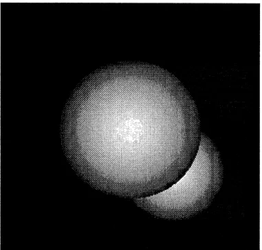
The third example relates to a sequence of occluding spheres shown in Figure 16. The

large sphere is expanding and the smaller one is translating southeast. The image presents

some difficulty because of the occlusion where the spheres overlap, and because of the

(15)

Figure 12: First frame of rotation sequence

x x X ~ ~ t I t I / ._ _ _ // , ,., .I , ,\ V /...-///././.,-.,- I - " - %%-~xNq I i i / , I /I x //l//l// -\\ - / I / / ' ' _/s x \ \ f f /// // // ... ..-....- / / / Is ! I \ '~\ x *, * * . f I J I zI J .1 / / //l/J / // f,lNit f t 1 J l l

Figure 13: Spatial gradient of previous image

13

, \ \ \ N X X

~~~~~Y~:i:~,,

, \ xs t

a~~~~~~ ' a X> __ wo/t / :t t t\ \ u x s 4 F t v > s w z / / / t / 1 1 t \ \ u \ sv _:I~:::~li::i::ii~ii: t.>?>s._ ::::::::`' ''::::

4~~~~~~~~~~, s s _ _ _ _ _ v / / : t .. ., : ·· ·: ' $ i , ,

~~~~~~~~~~::ii:

' ___oo /ft8t u> <

*~~~~~~~~~~~~~~~':i~~~~i~~i~~~iiiii * ._ __ __ -o / f t / /t 1 \ t \ N s x u > *~~~~~~~~~~~~~~~~t5 ·. _ _ + _ _ _ _ / / :: / f t / ./ f / / f ..: : :: : 2, · .~~~~~~~~~~~~~111 _ >__ r/ /// ttf 8\ \\^ ,, S > r o o , / / t t / f f t 8 \ \ t s s v v >·:·I··5'~: _ > _, _, . S

~s,i·:

r o fl o / · r:, :: : : : l : : : t t t s v s > ...

~~~~~~~~~~

.. ::;.: ···; ··I , ., t / / // J / fl ? P t + t \ \lW W * a + S < t s w E X X / / f \ v a s ? # # f t + rI a aI:I

Figure

Spatial gradient of:·.·· preio s image

13:

(16)

- - - - //''''''\\\\\\\4 441111 /- / ,l',~''''''\ . ... 1111 - -~rr'.rr(

~

\1 144111 441 ll l l l//////I/t f/tf f/fl' ...- ,ti t)il4/,l4//, f//ff jt ii4 , ,, - . ~, / //Ill Icr \'' ·''.'"//// / f//lilt i '''-i " · l t l --llll //}lJ'''l/ 1If ) t f t / ~ ~

~ ~ ~ ~

,,/ / ... / / --zz---cccCI//~~,

~///

j~ll l l lll ----

~-~c

/t . / / // / J / I . l

-Figr t4 loato lxml flo f~d *' " ''0,P . = ... 5 0

yr

~

ll///t////////r I~~

~~~

_t _tI I I -

~~~~~~

'

~~~~/1

/ / _{/ / /}*' '' _/4 _{/ I}...' _/i_/' //- -rr/

~

1 \\ \ ,/,,, -. ,,,-,...11 'kN",1"---- ... A,'-', ''' \\\\\4 4441444~\ f////If/If'··c trll j//////I f/f / / " 4 " "'"'...' f/If f/fc\\~ ,,,,.,-4', l/I/l.//I//I f/I f f .,,.- 44 ..- ,,.. ... ...-. ,/,, --,.-' ,,'" I II lt ,,,,44 ,, , , '. - .'-' .. ff//lI 4 44-'.-'''' _ll_{'---'-".'-.-,\\\}_' -.-f/i/ ,////// ',',"'" '/, /"-', /, / /\/\/\/I I

~

/ ///// /// //// /~~~~//,,/ ... -~-4--- --- J -/ / / / / / / / / / / / / / / / -~~~--~...---- - - ' - --, -, -, , / / / / / I --

~---////////

/ /, /, /, ., /, / /.

(17)

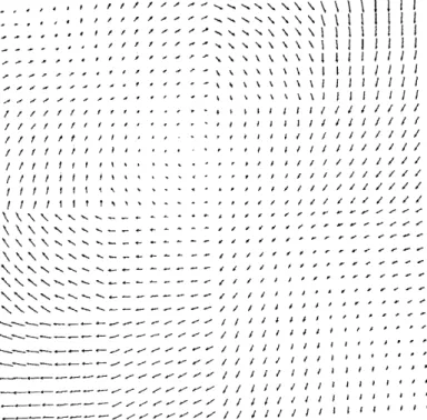
multiple motions. The actual optical flow is shown in Figure 17 and the flow computed with the tree algotihm is shown in Figure 18. The results of a number of experiments are presented in Table 4.

The smoothing of the optical flow across the boundary is typical of gradient based approaches [1]. The problem has been approached by doing segmentation prior to the es-timation process, so that only data within a segmented region affects the velocity estimate in that region [10]. One could imagine doing a similar thing with tree type models. Specif-ically, assume that some prior segmentation of the image is available into a set of regions. One could then estimate the flow in the regions separately by using a tree model prior for each. The resulting problem would likely have complexity similar to the original problem (after the segmentation is done) because the size of the segments would be much smaller than the image as a whole. Another approach to the problem would be to choose the tree model parameters in such a way that the regions found during the segmentation procedure were decorrelated in the prior model (it is assumed now that we are allowed to choose spatially and scale varying parameters). Whether or not this is easy to do depends on the nature of the segmentation. For instance, if there are four segments corresponding to the four quadrants then we can set the A matrix at the top level equal to zero (so that the first four branches coming off the root node are just equal to the driving noise, and the result is four decorrelated processes defined on trees one-fourth of the original size). But consider the (one-dimensional) situation depicted in Figure 19 where there are two regions that need to be decorrelated. In the figure, Ai denotes the transition matrix between the parent-child pair connected by the branch and i denotes the child node associated with that pair (so that node 4 is on the finest scale, third from the left). There are a number of possibilities for the segmentation in this case.

* Set A2 = A3 = 0. This decorrelates the two regions below nodes 3 and 1 as required,

but also decorrelates node 4 and the descendents of node 1 (and likewise for node 5 and the descendants of node 3), which is not desired.

* Set A3 = A5 = 0. This leaves the correlation structure of the left segment intact, and

decorrelates it from the right, but there is a loss of information from node 5.

* Set Al = A4 = 0. This is the same as above, but now the loss of information is

associated with node 4.

Of course, this does not exaust the possibilities. Instead of setting A matrices equal to zero, we could choose large driving noises. Also, information from any given node could be ignored by setting the noise variance parameter at that node artificially high. Variations on these methods may go a long way twoard solving the multiple motion/occlusion problem. The larger question here is what types of correlation structures can be realized with the quadtree model proposed, and given a particular correlation structure, how can it be realized? This is the stochastic realization problem for processes on trees, and is currently an open question. The fourth example is a synthetic fly through sequence of Yosemite. The image is shown in Figure 20 along with the actual flow field in Figure 21. The reconstructed flow is shown in Figure 22. This image contains a problem often encountered in real images: regions of constant intensity. The problem is that there is no gradient information in that region so that the optical flow is not well defined. The smoothness constraint of Horn and Schunk

(18)

Figure 16: Expanding and translating spheres : t ?J/... . . . . . . .\ .\ . . t t . / /. . . . . .. . . -. . . . . . . . I .J. , · 4 *' ~ . .~ . ....''. . , , _.., _/ _.._{k f f}I ._..' F \ \, \f _{I X\o\\} - -_NNN -' I I I I . - - . . .- , . '.' . . ' . '.' '. . . . . . . . . . . . . ..

(19)

.. < * . · · . · · ~ ~ *, . f f f f . . . ... .

<.

.

*.

;;.., .,\\\\ / 7/i/

I JN

Figure 18: Computed _... optical\ _\ \ _,\of sphere sequence a _\ / _II _{/ / ///, ...} 0.5, b 1 0.35

,./ I _ \ , Ji \ > xr\ '

.,

,,,,

?igute 18: Oomphted optical flow o _. tW,/ / K#'s\ \\\\\N9\\z sphere sequence a = 0,5, b = ]0, p = 0.35

* z/t / // / v\ \\\\\ \\\\

,iur 19 / OS / // / / ioa semntto \\ \XX p X\

(20)

Figure 20: First frame of Yosemite sequence

provides a means of interpolating out into these regions based on boundary values. The tree model also interpolates in these regions via the covariance structure induced by the prior model. The result of this is apparent in the top portion of Figure 22. Reconstruction and flow error data from four experiments are given in Table 5.

The fifth example is a sequence of automobiles and has examples of rotation, camera zoom, translation and a combination of translation and rotation. The gray scale image is shown in Figure 23 and the actual optical flow is shown in Figure 24. The computed optical flow is shown in Figure 25 (the flow was computed on each 128x 128 sub-image separately.) The parameters used were the same for all four sub-images and are the same as those used to compute the Yosemite optical flow shown in Figure 21. Four experiments were done for each sub-image of the car sequence; the numerical results on the flow reconstruction and frame reconstruction are provided in Table 6.

3 Surface Reconstruction

In this section the results of applying the tree smoothing algorithms to surface reconstruction problem are illustrated via a number of real and synthetic images. The first experiments utilize data generated from the tree model and are meant to illustrate the potential of the algorithm to deal with sparse and multiscale measurements. The second set deals with the Lena image and the third with a weather satellite image.

(21)

. / .. . . . . . .- . .-.-. . .-.-.-. .9. 9 9 9 1 -. / - -/- - ./ .-_ ./ -. 9 -. 9 ./ -/ / . / . . . . .// / ,//_ / / / / / / //// / / / /// I l II/ 4 ///99' ,/// //// / / / / / / I / / / / 4 //////////////// _/////////// _/_I/ _1/ _{/ / /}/ / / / _/I / / I _/_{1 1} I 4 _. 4 * _. _. 4 4 #////////////// / / / / / I/JI I J I I II //,/////////// / /J / 1 /J / / I I IIl 1 1 1\ \

Figure 21: Actual optical flow of Yosemite sequence

- - - - -. , / / , / t . . . .

- - - -- - - . . . .

-.7.9-9/////////

/ / 44 4444

///////// ///s/7 7,7// //" ///"/-79-9- 9

~

1"/ / ... / (i4 ... * I .*. . ... 1 * *

(22)

Figure 23: First frame of car sequence

-\ `` * \ \Z- I I ///-1 , - _1-.

*- -u \ // / I \ \N/.-IK

. .. .... . . . . _ .

i//Il....

\\\\\.

...

(23)

* _t -

~

. ', v \\ _{I/ ///}_{\ \} \ Xt

~

\\ " '>'> ,,,,, _- \ _ / /, I I / / / -\, ! /-- / / /// ~ ~ x ~ A \ \ .. Xv / -l -1-~~

~

.. \ It . // \ /_ d, -\ . -. \ \ i

,N,,.-..

.

...

,

x

X

-

,/

i_

Figure 25: Computed optical flow of car sequence a = 1, b = 1, y = 0.7

3.1 Surface Reconstruction using tree models

Again we make the assumption that measurements are available of a tree process and the smoothing algorithm is used to compute an estimate of the original image. The images are modeled as scalar processes, so that we must choose scalars corresponding to the parameters

A, B, C, t, and R. We make the assumption that the noisy data really is just the actual

image plus noise, thus C = 1 in the measurement equation (2). Also, we assume that the additive noise can be estimated from the image itself (by averaging over some region of constant intensity) so that the noise variance R is known. In general, the image could be modeled as the output of a vector tree process with arbitrary driving and measurement noises; we choose this simple case to limit the number of parameters that need to be chosen to three.

Again, the choice of a metric to ascertain how well the tree smoother works is important. In the examples below in which real images are analyzed we compare performance by presenting the reconstructed images and by comparing the improvement in the signal-to-noise ratio (SNR). This is defined as:

SNR =

Z(E(,

y) - E)2(20)

E(E(x, y) - E(x, y))2

(24)

Figure 26: Noisy measurements of Figure 2, SNR = 4/3

3.2 Examples

3.2.1 Synthetic Images

In the first example we use the sample path shown in Figure 2. Figure 26 shows the sample with noise added (n(t) - Af(O, 1); SNR = 4/3) and Figure 27 shows the smoothed estimate. Note here that most of the large discontinuities have been resolved, while detail has been lost at the finer scales. As one expects intuitively, the coarse scale features are better estimated than the fine scale variations. Another thing to note is that while this is indeed a smoothed estimate, the estimate is not smooth. This is possible because the smoothing is non-stationary. For a general set of data, the tree smoothed estimate of the underlying process will depend on where the tree process is assumed to lie.

We also illustrate how the smoother can be used to fuse multiscale information, and deal with sparse measurements. Figures 28 and 29 illustrate sparse measurements of the process at the finest scale and full coverage measurements at the fourth level (16 nodes), respectively. The sparse measurements are simply the original fine scale measurements restricted to a 16 pixel border around the image. Figures 30 and 31 show the resulting smoothed estimates given only the sparse measurements and both the sparse and coarse measurements, respectively. Note that the coarse data provides the smoother with some additional information about the middle of the process, and this is exhibited in the increased detail in this region in Figure 31 as compared to Figure 30.

(25)

Figure 27: Smoothed estimate of Figure 2

(26)

Figure 29: Coarse noisy measurements of Figure 2

(27)

Figure 31: Smoothed estimate of Figure 2, given sparse and coarse measurements

3.2.2 Real Images

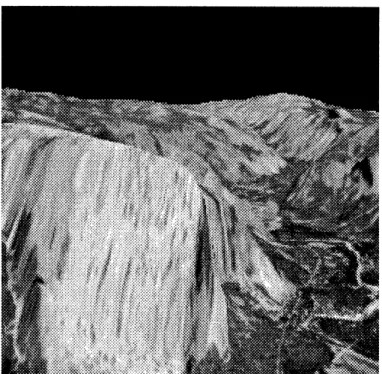
The previous examples were biased in favor of the tree smoother since the process really was a tree process, and the parameters required to do the smoothing were assumed to be known. More realistically, we would like to investigate how rich the processes are by smoothing examples of other non-tree processes, and comparing the results to standard smoothers. In the examples below we compare the tree smoother to a Gaussian lowpass filter in terms of signal-to-noise ratio improvement and visual appearance. The images used as a basis for comparison are the Lena image and weather satellite image of cloud cover.

Figures 32 and 33 are original and noisy versions of the Lena image (240x256). The noise is white Gaussian with mean zero and variance 400 (the original image has a sample variance of 2000 so that SNR = 5.0 in the noisy image). The tree smoothing algorithm was modified slightly to deal with the fact that the noisy image was not square - the noisy image was zero padded at the bottom with 16 rows. A somewhat better way to deal with the problem is to allow for spatially varying noise variances (i.e. allow R in the measurement equation to vary pixel by pixel). In regions of the quadtree where the image does not exist, zero pad and set the noise variance very high so that the false measurements are ignored.

Figures 34 and 35 show smoothed versions computed using the tree algorithm and a Gaussian lowpass filter. The Gaussian filter had support of 5 x 5, a variance of 0.65 and was normalized so that the sum of the filter coefficients over the support was equal to 1. The tree filter assumed a scalar process with A = 0.87, B = 70, C = 1, R = 400 and ,t = 0.37. These parameters were chosen because some experience indicated that they provided the

(28)

Figure 32: Original Lena image

nearly the best performance (in terms of SNR improvement) out of the class of Gaussian lowpass and quadtree smoothing filters respectively. The point is that we have tried to illustrate the best performance that both filters are capable of. The SNR's in the smoothed images are 13.6 and 18.3 for the tree smoother and Gaussian lowpass filter respectively.

Figures 36 and 37 are original and noisy versions of the weather satellite image (128 x 128). The additive noise is again white and normally distributed with variance 400 (the resulting SNR is 3.35). Figures 38 and 39 show smoothed versions computed using the tree algorithm and a Gaussian lowpass filter. The parameters of the filters were the same as in the previous example. The SNR of the tree smoothed estimate is 9.8 and that of the lowpass filtered image is 11.3. For comparison, the results of these two experiments and two others are shown in Table 7.

The performance of the tree smoother could be improved by allowing a more general parameter set (i.e. spatially and scale varying), which motivates the development of system identification tools for the tree process. The tree smoother may be most useful when mul-tiresolution measurements are available, in this case the tree smoothing algorithm provides a natural framework for combining the measurements. One key problem here is placement of the measurements on the tree, that is, deciding at what relative scales different sets of measurements may belong to. The current algorithmic structure assumes a dyadic sequence of scales. It would be useful to have a theory which allows for measurements at arbitrary scales.

(29)

Figu~~s:~:wwnre 3:

oiyLena

image

I.;

.:.. ' ..~.:.:::

~:~::. . . .

~

~~~~~~~~~~~~

*'.:~.~

'~~~; .4!!...:..

Figu.r e 34::Tree ima s t of Lena

27:i ====

!.!'i .' _{· ~:~::~::::::::::::::::::::::: :}. ' . . i~! ~:i!~!~!i::. ;; " _: _{. : i::~j}: i~...'::'!i_{':..~_.~}

i~i:~::!:!: .:-:'~:2:::$:::::!!~ii? . !.*~,' : :::..':::::: :.::~-:..============= = = ~.~.$::'~ ~'.?

~~~~~~~~

i·:....:::.::::::.::::'. : !.$~:: · ~::.' : : : : ' ,: ' ::~ :!

_~~~~~~:i!:'

~.:..i.i~ . ! : : ~~i!.~~ . ~~::" · ~! ~i~;

::.- ;:~i~.~~ ~:~i i.:-:+.:.:.::: :.

-~~~~::.~;.

Figure~ 34:

Ln

Te

mohdetmt

(30)

Figure

Lowpass filter estimate of Lena~~~~~~~~~~~::·:

35:

| | | | | | | | | ! | C

C

| s

|~~~~~~~~~~~~~:ii

r N E X g s X i S R S t t _ t~~~~~~~~~~~~~~~~~:·

o -| 11

| o | | | | | | | | l~~~b

_XO

_X

_O

₀₀

_{i 00}

_OXI

_#

_{I ·· :~::}

_{| ' Rs}

_R:

_·~e

_{_}

_'

| _ 11

ol x S l ox o l s | | l _

~;';5'.'"~·-~..i:·

S o oo > xo 0a #

::::.:dii~:ii'

0 gl X a < X 10 ' OC a -' _ -~~~~~~.· ao >: o eo > o

~~LX~i~s

xlS-is__-.

01 OE~gC~iE X s I: OOCODI SXio>XO se

I |

₁₁

11

_{i | I | E 0 0}

01 ! 11 | | 1|!

₀

_~:~st:

_{I ,0 |1}

_·jI

I

|

R5~~~~~~?.I

, I|

C pb.,*:g5 I_11l- iX~~~~~~~~~~~~~. OY X XilI IR:*::.¢.§6 l _ * l l _ - _ 11D _ OW '... X g. gl -l __ ^X~ _ >l_ 1 9-:': -l_ SO _ l § l~t~ gCQOIK l_ - - _ _ | _ g|I _Z l_- 11_X YOO c ll_ 1 -1l_ r~~Tgfaj _ m 11I*I - oo l o eo xwx 9 c l X l -l _ _ _ -i~iiiiiiii

~~

AW __f0ls w W w A v ff~~~~~~~~~~~:i B W _ S O | I _ | l * l _ -_

~:f·:·

X X<OOII 1|_XI-|___F

,0O

w>x K

elx11 l111 X I I XIOSII#63 l _ X 111 _11- :·t e xo o ool K10#10 1 I l 1 E l 11111 l 1-_ _ _acllll I K

~

#

~

WOO 0 : 3 ll l 11 s11 l _ _Y> :0XOsWf I 11l X X~~ X KII11

~

II OKI O l- l

e o o w l xaxo l l o s l N s _ _ _sI - WX X~~~~~~~~~~~~~~.:iiiijiiiii X OEI o _ K e w i XCI ffiD I K le | O~l O l II ilill_ l - _ _ RXII>C

X Cl 11 X XX 9GOI S I 1z_ lll I - I _ _ XlD:R4 1

r S K 3x I S * I 11S I _ IE Sg x~~~~~~~~~~~~~~~~~~~~~~~~~~~~~~~~~~~~~~~~~~~~~~~~~~il~i::iiiiiiii~fS

g~~~~ ,ii o I og i lgsI s

ez x xs l ooos nw l l s_ X l -oc·:;:s::l

* eeZ as l _- '>·Rw.

111 !X X s~~~~~::: iiiI I IXs' e-o;CS

(31)

Figure 37: Noisy satelite image

C|

E

| || ||

||

1 , 1 - E _ ' > 4x x > e c_ _~~~~~~~~~~::·:i

~:::::

· w w ' g -ES g e -_31~5~ ; S

111

11

, | .BW W N | 11 11|11 11 - - _~:~:

0 g

@1!

1

11 * * lli

-D

oXO

'

<

rz;

>

s

>

g

e

_~:5·

e

2X

:>

:::::.:<.::.

.::.::.:l

S_ S . | ,fi::Y *>W~ l|11 _ YX z > l mx @: .:: *. ^. :¢.- 2. +. lY | _ > P _~~~~~~~~~~~~~~~~~~~:··:I gg

~ ~~~~~~

l v

~

cov x:::.. *:.>.:::: *l E 5 Y MX n ; , : '. '. .:':.t'.4 .+.v':':'."::':'¢>, I . _IIIYY

Xiur 08 Tre ., : '''':::...'''"'".:#I* ote im t _ _aelt _m

(32)

Figure 39: Lowpass filter estimate of satellite image

4 Conclusions

This paper has described work in the area of two-dimensional multiscale signal processing. A new class of stochastic models and associated smoothing algorithms have been applied to the problems of optical flow, sensor fusion and surface reconstruction.

The results of the optical flow algorithms seem comparable to the results of the standard gradient techniques, although the regularization exhibits itself in a somewhat different way - there is a distinct blocky structure in the estimates. To what degree this is important depends on the application. For instance in motion based segmentation, the block structure may be a problem in so far as irregular boundaries would likely be missed. However, for applications such as motion compensated coding [2] or global motion identification [14] where smoothness is not an important issue, the quadtree based optical flow estimates may provide a means for obtaining good, fast solutions. Further work in the area of optical flow could move in a number of directions. First, there is the segmentation problem noted previously. A number of approaches to this problem have been suggested; the more general

problem is stochastic realization for the tree processes. Second, methods for obtaining

smoother estimates of the optical flow could be pursued. One simple way is to lowpass filter the tree based optical flow estimate. Another way would be to pursue estimation based on the more general lattice models. Finally, the application of the optical flow estimates to specific problems such as coding or motion interpretation could be pursued.

We have also applied the tree smoothing algorithms to the problems of sensor fusion, estimation based on sparse measurements and smoothing of real and synthetic images. It is

(33)

suggested that the real power of the tree smoother is in the natural framework it provides for sensor fusion. Further work in this area could move in two directions. First, the problem of choosing a set of parameters for the motivates the system identification problem for the tree processes. Second, the current algorithmic structure requires that the scales of different measurement sets are related by powers of two. Future work would remove this restriction, or provide some means for preprocessing the measurements to fit into the current structure. Finally, the more general lattice models provide a richer modeling structure that may lead to better reconstruction results, especially for fractal type images. Work in that area would also eventually lead to the system identification problem, as well as the previously discussed issues of scale.

(34)

Test a (A = aI) b (B =

bI)

IL RMS Flow error (x, y) RMS reconstruction error

1 0.5 10 0.35 -,- 0.21

2 1 10 0.7 -,- 0.24

3 1 10 0.35 -,- 0.20

4 1 20 0.35 -,- 0.20

Table 4: Sphere example parameters and performance criteria

Test a (A = al) b (B = bI) i RMS Flow error (x, y) RMS reconstruction error

1 0.5 1 0.35 0.20, 0.20 2.4

2 1 1 0.7 0.16, 0.14 2.1

3 1 1 0.35 0.17, 0.16 1.5

4 1 2 0.35 0.19, 0.19 1.2

Table 5: Yosemite flythrough example parameters and performance criteria

Test a (A = aI) b (B = bI) I RMS Flow error (x, y) RMS reconstruction error

NW 1 0.5 1 0.35 -,- 22.7 NW 2 1 1 0.7 -,- 12.0 NW 3 1 1 0.35 -,- 16.8 NW 4 1 2 0.35 -- 23.1 NE 1 0.5 1 0.35 -,- 14.0 NE 2 1 1 0.7 -,- 13.1 NE 3 1 1 0.35 -,- 14.5 NE 4 1 2 0.35 -,- 15.6 SW 1 0.5 1 0.35 -,- 17.2 SW 2 1 1 0.7 -,- 12.7 SW 3 1 1 0.35 -,- 12.7 SW 4 1 2 0.35 -,- 12.2 SE 1 0.5 1 0.35 -,- 27.5 SE 2 1 1 0.7 -,- 18.6 SE 3 1 1 0.35 -,- 16.4 SE 4 1 2 0.35 -,- 18.4

Table 6: Car sequence parameters and performance criteria

Test Noisy image SNR Tree smoothed image SNR Lowpass filtered image SNR

Lena 3.35 11.2 15.0

Lena 5.0 13.6 18.3

Clouds 3.35 9.8 11.3

Clouds 5.0 11.6 12.9

(35)

References

[1] Aggarwal, J., and Nandhakumar, N., On the computation of motion from sequences of

images - a review. Proc IEEE, 76:917-935, 1988.

[2] Baaziz, N. and Labit, C. Multigrid motion estimation on pyramidal representations for

image sequence coding. IRISA internal publication No. 572, February 1991.

[3] Burt, P., and Adelson, E. The laplacian pyramid as a compact image code. IEEE Trans. on Comm., 31:532-540, 1983.

[4] Chou, K., Willsky, A., Benveniste, A., Basseville, M., Recursive and iterative

estima-tion algorithms for multiresoluestima-tion stochastic processes. Proc. 28th IEEE CDC

confer-ence, Tampa, Dec. 1989.

[5] Chou, K. A Stochastic Modeling Approach to Multiscale Signal Processing. MIT Ph.d. Thesis, Dept. of EECS, May 1991.

[6] Enkelmann, W. Investigations of multigrid algorithms for the estimation of optical flow

fields in image sequences. Computer Vision, Graphics and Image Proc., 43:150-177,

1988.

[7] Geman, S. and Geman, D., Stochastic relaxation, Gibbs distributions and the bayesian

restoration of images. IEEE PAMI, 12:609-628, 1984.

[8] Heeger, D. J., Optical flow using spatiotemporal filters. Int. J. Computer Vision, 1:279-302, 1988.

[9] Heitz, F., Perez, P., Memin, E., and Bouthemy, P., Parallel Visual Motion Analysis

Using Multiscale Markov Random Fields. IRISA Internal Report.

[10] Heitz, F. and Bouthemy, P., Multimodal estimation of discontinuous optical flow using

Markov random fields. Submitted to IEEE Trans. on PAMI, Jan. 1991.

[11] Horn, B. K. P. and Schunk, B., Determining Optical Flow. Artificial Intelligence, 17:185-203, 1981.

[12] Konrad, J. and JuBois, E. Multigrid Bayesian estimation of image motion fields

us-ing stochastic relaxation. Proc. 2nd Int. Conf. Computer Vision, pp. 354-362, Tarpon

Springs Fla, Dec. 1988.

[13] Nagel, H. On the estimation of optical flow: relations between different approaches and

some new results. Artificial Intelligence, 33:299-324, 1987.

[14] Nicolas, H., and Labit, C., Global motion identification for image sequence analysis

and coding Proc. ICASSP 91, Volume 4, pp. 2825 - 2828.

[15] Rougee, A., Levy, B., and Willsky, A., An estimation-based approach to the

recon-struction of optical flow. Laboratory for Information and Decision Systems TEchnical

(36)

[16] Simoncelli, E. and Adelson, E. Computing Optical Flow Distributions Using

Spatio-temporal Filters. Vision and Modeling Group, MIT Media Laboratory, preprint, May

1991.

[17] Terzopoulos, D. Image analysis using multigrid relaxation methods. IEEE Trans. on PAMI, 8:129-139, 1986.

[18] Walker, D. and Rao, K. Improved pel-recursive motion compensation. IEEE Trans. on Communications, 32:1128-1134, 1984.

[19] Wornell, G. A Karhunen-Loeve like expansion for 1/f processes. IEEE Trans. on Inf. Theory, vol:pp, 1990.

Applications of two dimensional multiscale stochastic models Mark R. Luettgen.

January, 1992

LIDS-

P 2088

Research Supported By: