This may be the author’s version of a work that was submitted/accepted
for publication in the following source:
Perrin, Dimitri
& Duhamel, Christophe
(2013)
Efficiency of parallelisation of genetic algorithms in the data analysis
con-text.
In Yoshida, K & Seceleanu, C (Eds.)
Proceedings of the 2013 IEEE
37th Annual Computer Software and Applications Conference Workshops
(COMPSACW 2013).
Institute of Electrical and Electronics Engineers ( IEEE ), United States of
America, pp. 339-344.
This file was downloaded from:
https://eprints.qut.edu.au/82683/
c
Consult author(s) regarding copyright matters
This work is covered by copyright. Unless the document is being made available under a Creative Commons Licence, you must assume that re-use is limited to personal use and that permission from the copyright owner must be obtained for all other uses. If the docu-ment is available under a Creative Commons License (or other specified license) then refer to the Licence for details of permitted re-use. It is a condition of access that users recog-nise and abide by the legal requirements associated with these rights. If you believe that this work infringes copyright please provide details by email to [email protected]
Notice: Please note that this document may not be the Version of Record
(i.e. published version) of the work. Author manuscript versions (as
Sub-mitted for peer review or as Accepted for publication after peer review) can
be identified by an absence of publisher branding and/or typeset
appear-ance. If there is any doubt, please refer to the published source.
Efficiency of parallelisation of genetic algorithms in
the data analysis context
Dimitri Perrin
∗†and Christophe Duhamel
‡∗Centre for Scientific Computing & Complex Systems Modelling, Dublin City University, Dublin, Ireland. †Laboratory for Systems Biology, RIKEN Center for Developmental Biology, Kobe, Japan.
Email: [email protected]
‡LIMOS, CNRS UMR 6158, Universit´e Blaise Pascal, Clermont-Ferrand, France.
Email: [email protected]
Abstract—Most real-life data analysis problems are difficult to solve using exact methods, due to the size of the datasets and the nature of the underlying mechanisms of the system under investigation. As datasets grow even larger, finding the balance between the quality of the approximation and the computing time of the heuristic becomes non-trivial. One solution is to consider parallel methods, and to use the increased computational power to perform a deeper exploration of the solution space in a similar time. It is, however, difficult to estimate a priori whether parallelisation will provide the expected improvement. In this paper we consider a well-known method, genetic algorithms, and evaluate on two distinct problem types the behaviour of the classic and parallel implementations.
I. INTRODUCTION
There is a direct analogy between most data analysis prob-lems and optimisation probprob-lems. This derives directly from the motivation behind data analysis: extracting the maximum information from available data.
The challenges are therefore largely similar. It is often not possible to aim for an exact analysis of an entire dataset, be-cause of the complexity of the associated algorithms. However, if the required analysis can be formulated as an optimisation problem, it is possible to use all the existing approximate methods developed in that field.
When using such methods, one must strike a balance between the quality of the approximation and the computation time of the method. Parallel computing can assist in this process, in that it allows a more complete exploration of the solution space at a limited cost.
In this paper, we consider two data analysis problems that can be solved using genetic algorithms, and we evaluate the benefits of using a parallel implementation, depending on the problem structure and dataset size.
II. GENETIC ALGORITHMS
A. Classic implementation
Genetic algorithms are loosely based on evolution in nature and survival of the fittest elements only [1]. The general idea is to maintain a pool of solutions, to let these evolve, and to actively select the most interesting ones.
Solutions are encoded as chromosomes, and evolution oc-curs through operators that alter these chromosomes. Mutation corresponds to creating a new solution by changing the value at a single position of a randomly selected chromosome. Uniform mutation involves the generation of a binary boolean array m, and alteration of position i of the chromosome if and only if m[i] = true. Another bioinspired operator is the cross-over: two chromosomes are selected, and two new solutions are obtained by exchanging a section of their values. In the single-point cross-over, a random value j is generated, and all the values at position i ≥ j are exchanged. In the two-point cross-over, two random values j and k are needed, and all the values at position j ≤ i ≤ k are exchanged. Other operators may aslso be considered, for instance a local search starting for a given chromosome. This classically leads to memetic algorithms, (see e.g. [2] for details on these methods).
Restoration has to be defined whenever these operators can produce ill-formed offsprings. Its process depends on the encoding scheme and on the problem considered. It is discussed in the next Section for the two problems used as examples.
The pool of solutions doubles in size during the evolution phase. The next step, the selection phase, brings it down to its original size. It is also bioinspired, in the sense that better solutions have a higher probability of surviving to the next iteration. There are two main strategies: (i) deterministically keep the best solutions; (ii) have one-to-one tournaments between randomly selected solutions, where the probability to win is higher for the better solution, (and can be a function of the gap between the solution). It is often useful to consider hybrid approaches, i.e. to keep the very best solutions and organise tournaments for the remaining ones.
This process is repeated over k iterations. It is also possible to use other stopping criteria, such as a maximum number of iterations without improvement of the best solution, but these are not considered here. Overall, the algorithm can be therefore summarised as follows:
1) Initialise a population of s solutions. 2) Run k iterations, defined as:
a) Population evolution. Its size reaches 2s. b) Restoration of the newly created solutions. c) Selection phase, until the size is down to s.
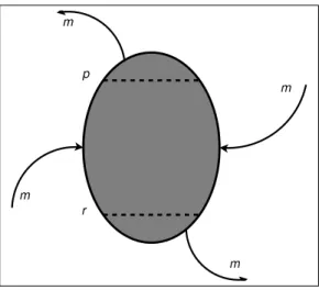
Fig. 1: Coarse-grained, stepping stone structure. Here, four subpopulations are connected through a bidirectional ring. Selected solutions are sent clockwise if they are selected from the “rich” area, and anti-clockwise if selected from the “poor” area.
3) Return the best solutions.
B. Parallel implementation
There are several way to parallelise a genetic algorithm. Here, we rely on the stepping stone model [3]. For migrations, each subpopulation is sorted according to its score, and two thresholds are used to define the “rich” and “poor” areas, (which contains the solutions with the best and worst scores, respectively). A bidirectional ring is then used to send solutions selected from these two areas. This topology is detailed in Figures 1 and 2.
One of the main advantages of this approach is that it scales easily to any number of subpopulations and can therefore be used on multi-core desktops or laptops as well as on high-end clusters or cloud environments.
The parallel algorithm can be summarised as follows: 1) Initialise n subpopulations.
2) Run k1 global iterations, defined as:
a) Run k2 local iterations, i.e. k2 iterations of
the classic implementation above. b) Sort each subpopulation.
c) Select and migrate solutions. 3) Return the best solutions.
III. DATA ANALYSIS PROBLEMS
In this paper, we consider two problems. While very different in nature, they are complex enough that exact methods are not suitable tools for realistic instance sizes.
p r m m m m
Fig. 2: Parallel topology. Before a migration step, each sub-population is sorted. Then, m solutions are selected from the most promising ones, (i.e. from those ranked below threshold r, assuming we have a minimisation problem), and are sent clockwise. Similarly, m solutions are selected from the least promising ones, (i.e. from those ranked above threshold p), and are sent anti-clockwise. Finally, new solutions are received: m good solutions arrive clockwise, and m poor solutions arrive anti-clockwise.
A. Microarray biclustering
Microarrays are used for large-scale transcriptional profil-ing, and measure expression levels of thousands of genes at the same time. The motivation is that, by understanding gene expression, further insight can be gained into cell function and cell pathology [4].
To analyse such datasets, one must cluster the data [5], i.e. group genes based on their expression under multiple condi-tions or, conversely, group condicondi-tions according to expression of several genes. Biclustering is a refinement of this technique, in that it corresponds to the simultaneous clustering of both genes and conditions [6].
Mathematically, this data can be treated as a bipartite graph. Genes and experimental conditions are two distinct sets, and edges exist only between all pairs formed by one gene and one condition, as shown in Figure 3. Assuming that each edge has a biologically relevant weight (see [7] for details), biclustering can be solved by an algorithm looking for bicliques with minimum total weight.
It is interesting to note that, in a typical microarray dataset, there are thousands of genes and a few dozens conditions. Let us consider a given subset of conditions. The best solution for this subset is clearly the one obtained by selecting all genes for which the total weight over the selected conditions is negative and leaving out all the other genes. This is a simple operation, so it is only necessary to encode the condition subset in the chromosome. The added benefit is that no repair function is needed. The rest of the algorithm is unchanged.
genes
conditions
Fig. 3: A biclique with 3 genes and 2 conditions in a complete bipartite graph with 6 genes and 5 conditions.
datasets over increasing complexity1: (i) a Kasumi Cell Line (KCL) dataset [8] with 22283 genes and 10 conditions; (ii) a Yeast Cell Cycle Data (YCC) dataset [9] containing time-course expression profiles over 6000 genes, with 17 time points for each gene; (iii) a Lymphoma (L) dataset [10] with 4026 genes and 96 conditions.
B. Minimum size convex hull
The problem we are considering can be described as follows: given a set of n points in a 2D space, find the subset of size k whose convex hull has a minimum size2. An example
is shown in Figure 4. Using the genetic algorithm described earlier, we get solutions for all k ∈ J1; nK. Here, we use standard encoding: the chromosome length is n and, for any point j ∈J0; n − 1K, Ci[j] = 1 if j is in the subset of points
encoded by chromosome Ci, and Ci[j] = 0 otherwise.
Chromosome restoration and evaluation starts by comput-ing the convex hull of the encoded solution, uscomput-ing Andrew’s algorithm [11]. Then, points that are located inside the hull but were not included in the solution are added to the subset. Finally, we compute the size of the subset and the hull size3. The rest of the algorithm is as introduced earlier.
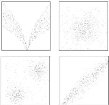
The main difficulty in this problem is the number of points, as the number of possible solutions grows exponentially with the dataset size. Here we consider datasets with 25 to 1200 points, generated using various probability distributions and combinations of these, as shown in Figure 5.
IV. RESULTS
The main objective of our paper is to compare the perfor-mances of the two implementations of the genetic algorithm, and to identify whether parallelisation is always a worthwhile alternative. Our focus is, therefore, not primarily on whether the optimal solution can be identified, but rather on the gap between the solutions and between the execution times.
1The most significant contributor to making these datasets difficult to
analyse is the number of conditions. We do not detail this here, but the discussion on chromosome encoding gives an initial justification.
2Several versions of the problem exist: minimisation of the area, the
perimeter, or a sum of the two. Here, we focus on the last one but the results are applicable to all versions.
3We do not need to compute the hull again: any point added to the subset
during restoration is strictly inside the hull.
Fig. 4: A set of 25 points and a solution with 10 points. Note that 7 points are on the hull itself, whereas the other are inside and must be identified during restoration.
Fig. 5: Examples of 1200-point datasets used for the minimum area convex hull problem.
For the two problems under consideration, there are two criteria to evaluate a solution: its value and its size. This does not, however, correspond to multi-criteria optimisation. Here one only criterion, the value of the solution, is optimised, whereas the other one is explored. This is why the genetic algorithm does not use notions such as Pareto dominance. For a problem of size n, the genetic algorithm directly returns n solutions:
• for a microarray with n conditions, the best bicluster it found with exactly k active conditions, with k ∈ J1; nK.
• for a dataset with points n in the hull problem, the best subset with exactly k points, with k ∈J1; nK. Comparing the solutions obtained by the various ap-proaches is not trivial. For large problems, improving a specific region of the solution profile may go unnoticed if we only look at the average solution improvement. A number of metrics can be considered, but we have selected three that are both significant and easy to interpret:
• Mi: the maximum gap between a solution sc (of
any size) found by the classic implementation and a solution si of same size found by a parallel
imple-mentation using i islands.
• Ai: the average value of the gap between sc and si.
• ∆: the average, over all k ∈ J1; nK, of the standard deviation of the value found for the solution of size k (calculated over ten repeats of the genetic algorithm). To facilitate analysis across problems, ∆ is given as a percentage of the average solution.
Some additional details on the gap between sc and si are
needed. In the microarray problem, all solutions have, by construction, a negative weight. Thus, better solutions have a higher absolute value. For the hull problem, the opposite configuration occurs, as we work with the area and perimeter. As a result, to improve the analysis across problems, we define the gap as the ratio si/sc for the microarray problem, and as
the ratio sc/si for the hull problem.
Both problems have been tested a two architectures: a 2008 448-core cluster computer (56 compute nodes with dual quad-core 2.66Ghz processor and 8Gb memory, InfiniBand interconnect) and a 2012 desktop computer (quad-core 3.1GHz processor, 16Gb memory). While the absolute computing time varies4, the trends in relative computing time when using the
parallel implementation and increasing the number of islands are conserved.
A. Microarray biclustering
Table I summarises the average computation time on datasets of increasing sizes for the microarray problem. The standard deviation observed over ten runs is below 1.2% for all configurations, so these average times are statistically significant. The cost of using eight islands instead of a single population (and therefore working with eight times as many
4The more recent desktop is faster in our tests, but the cluster has the
advantage of being able to handle a larger number of islands if necessary for specific problems.
solutions) is very low, between 7.8% and 13.6%. The total computation time is lower for the 17-condition problem than for the 10-condition because, even though the former dataset is more complex to analyse, it contains far fewer genes than the latter (6,660 instead of 22,283) and evaluation of each solution is therefore faster.
The more complex a dataset is, the larger the improvement provided by the parallel implementation becomes. This is shown in Table II, and applies to both the average gap, 5%– 24%, and the maximum gap, 132%–259%. The 10-condition problem is a special case: the dataset is small enough that both implementations find the optimal solution, for each bicluster size, at each run. This was verified using a dedicated exact method and implies that the parallel implementation can not give any improvement for this dataset.
A better exploration of the solution space also means that the most interesting regions are identified more frequently. A direct consequence is that the standard deviation of the solution value is reduced when the number of islands is increased, as shown in Table III. As previously, the difference becomes more significant for more complex datasets.
Pb. size Classic 2 islands 4 islands 6 islands 8 islands 10 1.00 1.03 1.08 1.10 1.13 17 0.81 0.84 0.89 0.90 0.92 96 17.76 17.97 18.47 18.81 19.15
TABLE I: Computation time for the microarray problem. Results are given relative to the computation time for the 10-condition problem with the classic implementation.
Pb. size 2 islands 4 islands 6 islands 8 islands 10 (1.00; 1.00) (1.00; 1.00) (1.00; 1.00) (1.00; 1.00) 17 (1.05; 1.32) (1.08; 1.35) (1.09; 1.45) (1.09; 1.45) 96 (1.09; 2.21) (1.19; 2.53) (1.21; 2.57) (1.24; 2.59)
TABLE II: Results for (Ai; Mi) for the microarray problem.
Pb. size classic 2 islands 4 islands 6 islands 8 islands
10 0.0 0.0 0.0 0.0 0.0
17 7.3 5.4 2.7 1.4 1.6
96 18.2 12.12 8.31 7.00 5.95
TABLE III: Results for ∆ for the microarray problem.
B. Minimum size convex area hull
Table IV summarises the average computation time on datasets of increasing sizes for the hull problem. The standard deviation observed over ten repeats is between 1.5% and 6.5%, so these average values can used with confidence. The results confirm that the parallel genetic algorithm scales well: going from two to eight islands (and therefore working with four times as many solutions) only increases the computation by a factor of 1.8.–2.5, while the overhead of the 8-island parallel algorithm compared to the classic approach is only 2.0–2.9.
While very satisfactory, the performance is not as good as for the microarray problem. This is a result of solution encoding. In the microarray problem, it was possible to find an
encoding that removes the need for solution restoration. Each iteration only involves evolution and selection, and the load is therefore very evenly balanced across processes. In the hull problem, restoration is needed, and takes a time proportional to number of points located directly on the hull, (and not the size of the subset). We think this creates imbalance in the load, and therefore reduces the computing performance, (as the migration step requires synchronisation).
In terms of the solutions obtained by the algorithm, the parallel implementation always outperforms the classic imple-mentation. Table V shows the results in terms of average and maximum gap between the classic and parallel implementa-tions. A higher number of subpopulations lead to a better exploration of the solution space. New solutions are identified, highlighted by high values for Mi, often over 200%. For
this problem, some solutions are trivial (i.e. subset with very few points, or almost all points). Optimal values are easily identified for such subsets, and this explains why Ai shows
little improvement as i increases.
A better exploration also means that these good solutions leading to high Mi values are more frequently identified, and
this leads to reduced ∆ values when i increases, as shown in Table VI.
Pb. size Classic 2 islands 4 islands 6 islands 8 islands 25 1.00 1.15 1.34 1.72 2.10 50 1.92 2.04 2.71 3.24 3.90 75 3.08 3.32 4.12 5.25 6.34 100 4.16 4.40 5.34 7.28 8.50 500 23.91 26.92 34.34 46.59 59.41 1000 56.12 64.66 87.29 125.73 164.69
TABLE IV: Computation time for the hull problem. Results are given relative to the computation time for the 25-point problem with the classic implementation.
Pb. size 2 islands 4 islands 6 islands 8 islands 25 (1.00; 1.02) (1.01; 1.13) (1.01; 1.13) (1.01; 1.13) 50 (1.08; 3.30) (1.09; 3.30) (1.09; 3.30) (1.10; 3.30) 75 (1.01; 1.12) (1.02; 1.27) (1.04; 1.78) (1.05; 2.21) 100 (1.02; 1.56) (1.03; 1.63) (1.05; 1.81) (1.05; 1.75) 500 (1.01; 1.37) (1.02; 2.72) (1.03; 4.70) (1.04; 4.12) 1000 (1.01; 1.40) (1.02; 2.24) (1.02; 2.41) (1.03; 3.47)
TABLE V: Results for (Ai; Mi) for the hull problem.
Pb. size classic 2 islands 4 islands 6 islands 8 islands 25 1.09 0.83 0.24 0.16 0.10 50 6.90 1.83 1.76 1.60 1.20 75 2.70 2.17 2.11 2.06 1.72 100 3.23 2.23 2.00 1.85 1.91 500 1.69 1.56 1.51 1.46 1.40 1000 1.54 1.48 1.30 1.22 1.10
TABLE VI: Results for ∆ for the hull problem. Given that the average improvement Aiis limited, a second
parallelisation strategy can be considered. Previously the algo-rithm used, for each island, the same population size that would be used with the classic implementation. Another approach would be to divide that original population size across the islands.
This means switching the focus from a better exploration of the solution space to a reduced computation time. It could be a useful strategy in case where the average solution (or the overall solution profile) is more important that the best solution.
To investigate the impact of this second strategy, we use a dataset with 1200 points, and total pool of 240 solutions. This means that each island has 120 solutions when running the parallel implementation on two computing nodes, 60 with four nodes, 40 with six nodes, and 30 with eight nodes.
We used the same metrics as for the initial strategy (i.e. relative computation time, Ai, Mi and ∆), and report the
results in Table VII. We can see that, as long as the overall population is kept constant, the results are not significantly altered by using several islands: Ai is almost unchanged, and
the increase in ∆ is limited. The increase in Mi should not be
considered as an advantage of the parallelisation strategy: here, it is an artefact of the increased variability and, while some solutions are improved, others are degraded, as highlighted by the fact that Ai is constant.
The results are mostly unchanged, but the required time to obtain these is significantly reduced. For this dataset, the optimal configuration was to use four islands, (computation time reduced by 56%). Theoretically, in a perfectly-balanced system, a larger number of islands should give better results. As we described earlier, the restoration method for this specific encoding of the hull problem creates load imbalance, and this explains why the computation time increases again for large numbers of islands.
Metrics Classic 2 islands 4 islands 6 islands 8 islands Rel. time 1.00 0.54 0.46 0.55 0.68 Ai N/A 0.997 0.997 0.998 1.002
Mi N/A 1.410 1.144 1.339 1.656
∆ 1.85 1.94 2.06 1.99 1.91
TABLE VII: Evaluation of the second strategy.
V. CONCLUSION
The analysis of large datasets is not trivial, but the process can be improved by using techniques derived from Operations Research. In this paper, we showed how two well-known examples can be considered as optimisation problems.
Once formulated as such, it is possible to solve these using a genetic algorithm. We proposed a parallel implementation of the algorithm, and evaluated the benefits of such an approach. Depending on the problem, two strategies can be considered: 1) Using the parallel structure to increase the population
size, and therefore better explore the solution space. 2) Working with a constant population size and using the parallel structure to divide this population into smaller subsets that are faster to process.
Our evaluation confirmed the potential of parallel genetic algorithms, but also highlighted that solution encoding can lead to load imbalance, and must therefore be carefully considered.
ACKNOWLEDGMENTS
Some of the parallel implementations discussed in this paper were tested on the cluster made available by the Centre for Scientific Computing & Complex Systems Modelling, Dublin City University.
Financial support from the Irish Research Council for Science, Engineering and Technology (IRCSET), co-funded by Marie Curie Actions under FP7, and subsequently from the RIKEN Foreign Postdoctoral Researcher Program, is warmly acknowledged (DP).
REFERENCES
[1] J. H. Holland, Adaptation in natural and artificial systems. MIT Press, 1975.
[2] F. Neri and C. Cotta, “Memetic algorithms and memetic computing op-timization: A literature review,” Swarm and Evolutionary Computation, vol. 2, pp. 1–14, 2012.
[3] E. Cantu-Paz, “A summary of research on parallel genetic algorithms,” IlliGAL report 95007, vol. University of Illinois (IL), 1995.
[4] F. Valafar, “Pattern recognition techniques in microarray data analysis: A survey,” Annals of the New-York Academy of Sciences, vol. 980, no. 1, pp. 41–64, 2002.
[5] G. Stolovitzky, “Gene selection in microarray data: the elephant, the blind men and our algorithms,” Current Opinion in Structural Biology, vol. 13, pp. 370–376, 2003.
[6] Y. Cheng and G. M. Church, “Biclustering of expression data,” in Proceedings of the 8th International Conference on Intelligent Systems for Molecular Biology (ISMB 2000), vol. 8, San Diego, California, USA, August 2000.
[7] G. Kerr, D. Perrin, H. J. Ruskin, and M. Crane, “Edge weighting of gene expression graphs,” Advances in Complex Systems, vol. 13, no. 2, pp. 217–238, 2008.
[8] Gefitinib Treated Kasumi Cell Line Dataset, MIT Broad Institute, “http://www.broad.mit.edu/cgi-bin/cancer/datasets.cgi.”
[9] Yeast Cell Cycle, available from R.W. Davis’ website at Stanford, “http://genomics.stanford.edu/yeast cell cycle/cellcycle.html.” [10] Lymphoma/Leukemia Molecular Profiling Project Gateway,
“http://llmpp.nih.gov/lymphoma/.”
[11] A. M. Andrew, “Another efficient algorithm for convex hulls in two dimensions,” Information Processing Letters, vol. 9, pp. 216–219, 1979.