Applicability of deep learning approaches to non-convex optimization for trajectory-based policy search

Applicability of Deep Learning Approaches to

Non-Convex Optimization for Trajectory-Based

Policy Search

by

Robert Verkuil

Submitted to the Department of Electrical Engineering and Computer

Science

in partial fulfillment of the requirements for the degree of

Master of Engineering in Electrical Engineering and Computer Science

at the

MASSACHUSETTS INSTITUTE OF TECHNOLOGY

February 2019

Massachusetts Institute of Technology 2019. All rights reserved.

Author ...

Signature redacted

Department of Electrical Engineering and Computer Science

Signature redacted

February 4, 2019

Certified by...

Russell L. Tedrake

Professor

Thesis Supervisor

Accepted by ...

MASSACHUSETS INSTIUTE OFTECHNOLOGY

rFEB

2 7

019

LIBRARIES

Signature redacted

Katrina LaCurts

Chair, Master of Engineering Thesis Committee

77 Massachusetts Avenue

Cambridge, MA 02139

MITLibranies

http://Iibraries.mit.edu/ask

DISCLAIMER NOTICE

Due to the condition of the original material, there are unavoidable

flaws in this reproduction. We have made every effort possible to

provide you with the best copy available.

Thank you.

The images contained in this document are of the

best quality available.

Applicability of Deep Learning Approaches to Non-Convex

Optimization for Trajectory-Based Policy Search

by

Robert Verkuil

Submitted to the Department of Electrical Engineering and Computer Science on February 4, 2019, in partial fulfillment of the

requirements for the degree of

Master of Engineering in Electrical Engineering and Computer Science

Abstract

Trajectory optimization is a powerful tool for determining good control sequences for actuating dynamical systems. In the past decade, trajectory optimization has been successfully used to train and guide policy search within deep neural networks via optimizing over many trajectories simultaneously, subject to a shared neural network policy constraint.

This thesis seeks to understand how this specific formulation converges in compar-ison to known globally optimal policies for simple classical control systems. To do so, results from three lines of experimentation are presented. First, trajectory optimiza-tion control soluoptimiza-tions are compared against globally optimal policies determined via value iteration on simple control tasks. Second, three systems built for parallelized, non-convex optimization across trajectories with a shared neural network constraint are described and analyzed. Finally, techniques from deep learning known to improve convergence speed and quality in non-convex optimization are studied when applied to both the shared neural networks and the trajectories used to train them.

Thesis Supervisor: Russell L. Tedrake Title: Professor

Acknowledgments

This thesis would not have been possible without the support and encouragement of many people, whom I would like to thank immensely.

To my thesis advisor, Russ Tedrake, thank you for all of your guidance, especially throughout the evolution of this thesis. In my undergraduate years, I always enjoyed our conversations about life and your work. Getting the opportunity to be a part of your group has been just as exciting and fulfilling as it seemed to the wide-eyed sophomore who stepped into your office those several years ago.

To Eric Cousineau, Greg Izatt, Hongkai Dai, Pete Florence, Robin Deits, Tobia Marcucci, Twan Koolen, and all my other lab mates, thank you for always being open to discussions about your work, for answering my many questions, and for showing me how fun it is to think about and play with robots all day.

To all my friends who gave me advice, encouraged me, and went far out of their way to help me during this past year, thank you. I could not have done this without you.

Finally, to my Mom, Dad, and sister - thank you for your unending love. During those long nights, it was always the thought of your unconditional support that gave me the strength to find a way forward, and to imagine an amazing future.

Contents

1 Introduction

15

1.1 A pproach . . . . 16 1.2 C hallenges . . . . 17 1.3 Contributions . . . . 18 1.4 Thesis O utline . . . . 18 2 Related Work 21 3 Adding Neural Network Support to Our Optimization Toolbox 25 3.1 Background on Drake . . . . 26

3.2 D esign . . . . 28

3.3 Custom Constraints and Costs . . . . 30

3.4 Implementation and Evaluation . . . . 32

3.4.1 Memory usage analysis . . . . 32

4 Understanding Simple Dynamical Systems With Value Iteration 35 4.1 Value Iteration Background . . . . 35

4.2 Introducing The Tasks . . . . 36

4.2.1 Our Desired Experiments . . . . 37

4.2.2 Experiment 1: Visually Inspecting Value Iteration Results . . 37

4.2.3 Experiment 2, Evaluating Minimum Neural Network Sizes for Fitting Value Iteration Policies . . . . 39

4.3.1

Direct Transcription and Direct Collocation . . . .

4.4 Experiments relating Trajectory Optimization and Value Iteration . . 4.4.1 Comparing Cost-to-Go and Policy Obtained from Value Itera-tion and Trajectory OptimizaItera-tion . . . . 4.4.2 Effect of Warm Starting on the Divergence of Trajectory Opti-mization vs. Value Iteration Costs-to-Go and Policies . . . . . 4.5 C onclusion . . . .

5 Constrained Trajectory Optimization - Setup

5.0.1 Recap and Motivation . . . . 5.0.2 Chapter Focus . . . . 5.1 Simple Approach .... ...

5.1.1 Issues with the Simple Approach . . . . 5.1.2 Benefits of the Simple Approach . . . . 5.1.3 Applying the Simple Approach to Pendulum Swing-up

5.1.4 Applying the Simple Approach to Cartpole Swing-up 5.2 Fully Constrained Approach . . . .

5.2.1 D esign . . . . 5.2.2 Scaling Evaluation of the Fully Constrained Approach .

5.2.3 Parallel Implementation . . . . 5.3 Block-Alternating Approach . . . .

5.3.1 D esign . . . . 5.3.2 Parallel Implementation . . . .

6 Constrained Trajectory Optimization - Experiments

6.0.1 O utline . . . . 6.0.2 Relating this chapter to earlier experiments. . . . . 6.1 B aselines . . . . 6.2 M ini-Batching . . . . 6.3 D ropout . . . . 6.4 Further observations . . . .

41

42

43

46

50

51

. . . .

51

. . . .

51

. . . .

54

. . . .

54

. . . .

55

. . . .

56

. . . .

58

. . . .

59

. . . .

59

. . . .

60

. . . . 61

. . . .

62

. . . . 63 . . . . 63 65

. . . .

65

. . . .

65

. . . .

66

. . . .

66

. . . .

68

. . . .

69

6.4.1 Added Gaussian Noise . . . . 69 6.4.2 Interaction of Dropout and Gaussian Noise with the Optimizer 69

7 Conclusion

71

List of Figures

3-1 Flow chart of the logic within NNSystem. . . . 29

3-2 Timeline diagram showing where time is spent in evaluating a neural network policy constraint. . . . . 33

4-1 Double Integrator System . . . . 36

4-2 Pendulum System . . . . 36

4-3 Cartpole System . . . . 37

4-4 Value Iteration vs. Trajectory Optimization Results for Double Inte-grator ... .. .. ... 38

4-5 Value Iteration vs. Trajectory Optimization Results for Pendulum . . 39

4-6 Double Integrator Cost to Go Comparison . . . . 43

4-7 Double Integrator Policy Comparison . . . . 44

4-8 Pendulum Cost-to-Go Comparison . . . . 45

4-9 Cost-to-go vs. Policy Discrepancies for Double Integrator . . . . 47

4-10 Cost-to-go vs. Policy Discrepancies for Pendulum . . . . 48

4-11 Cost-to-go vs. Policy Discrepancies for Cartpole . . . . 49

5-1 Key of symbols used in system diagrams to come. . . . . 53

5-2 Diagram of Simple Approach . . . . 54

5-3 Example of Pendulum Policy Inconsistency . . . . 55

5-4 Policy rollouts from random initial conditions (blue) to end state (purple). 56 5-5 Comparison of Policies from Value Iteration and Simple Approach . . 57

5-6 Cartpole Partial Success with Simple Approach . . . . 58

5-8 Scaling Fully Constrained Approach . . . . 60

5-9 Diagram of Parallel Fully Constrained Approach to Shared Policy Op-tim ization . . . . 61

5-10 Diagram of Block-Alternating Approach . . . . 62

6-1 Value Iteration Policy vs No Mini-batching vs Mini-batching . . . . . 67

6-2 Reference Pendulum Swing-up Policy from Value Iteration . . . . 68

6-3 Examining the effect of adding dropout to the learned policy. . . . . . 68

6-4 Training curves reporting mean average error over randomly selected points in the state space w.r.t. known optimal from value iteration, with and without dropout. . . . . 69

List of Tables

4.1 Minimal Neural Network Testing to Fit Optimal Policies from Value Iteration . . . . 40 A.1 Value Iteration Settings . . . . 73

Chapter 1

Introduction

Trajectory optimization is a powerful tool for determining good control sequences for actuating dynamical systems. A key to its ability to find good controls in high-dimensional, real-world state spaces is that optimization is only done over a single sequence of states and actions over time, from a fixed initial state. These state-action pairs, or 'knot points', are the discretization over time of the otherwise continuous-valued trajectory and serve as the decision variables for the optimization. Because of this discretization over time and restriction to a single starting state, trajectory optimization can scale in environments with state dimensions where calculating a globally optimal feedback controller is computationally infeasible.

Trajectory-based policy search algorithms like Guided Policy Search [6] and related works [7], [8], [10], [111, are a class of algorithms that seek to harness the power of trajectory optimization to find good control sequences in complex environments to train flexible policies that can be applied outside of a single trajectory. To do

so, these algorithms jointly optimize over multiple trajectories, either to provide a

guiding distribution for fitting a neural network in a separate optimization stage, or to directly train the network via costs/constraints imposed at each knot point along the trajectories. For example, a constraint may be declared for every knot point in each trajectory, fixing the knot action as being equal to the policy's output, given the knot state.

tasks like swinging a torque-limited pendulum or cart-pole into its upright position. When combined with the very nonlinear structure of a neural network and distributed training architecture where parameters updates can not be synced at all times, its very interesting to look at the techniques researchers have used to still converge to good policy solutions.

1.1

Approach

We take the following three pronged approach towards understand the convergence properties of policy-constrained trajectory optimization.

Prong 1: We'd like to build and understand issues with scaling and convergence with truly-constrained shared policy trajectory optimization. To do so, we will for-mulate a large nonlinear optimization problem containing decision variables for the knot points of many trajectories, and decision variables for a neural network. We make heavy use of the optimization toolbox, Drake, developed by researchers in the Robot Locomotion Group at the Computer Science and Artificial Intelligence Labora-tory at MIT. Drake has tools for many attractive variants of trajecLabora-tory optimization, and supports powerful solvers that can accept user-defined functions for costs and constraints.

Prong 2: In case prong 1 has difficulty scaling to environments more compli-cated than the torque-limited pendulum, e.g. the cart-pole task, we'd like to explore an alternative algorithm that permits better scaling at the cost of less convergence guarantees. This algorithm will take a block-alternating approach that first optimizes over trajectories with a shared policy cost rather than a constraint. During this stage the neural network parameters will be frozen, and so the trajectory optimizations will be trivially parallel among CPU cores. In the second step of the block alternating approach, we will perform simple supervised learning on the trajectories. To encour-age the trajectories and neural network to "co-adapt", we will carry out a limited number of iterations in each phase, and can add proximal cost terms discouraging each optimization phase from being able to make too much progress. This approach

is inspired by the paper "Interactive Control of Diverse Complex Characters with Neural Networks" [11].

Prong 3: To aid in our design and experimentation with prongs 1 and 2, we'd

like to understand the globally optimal controllers for our simple control tasks, which can be determined exactly when state dimensions are low, via the algorithm of value iteration. In value iteration, the state and action space is discretized, and a cost-to-to is calculated recursively via one-step transitions from each state to its neighbors, via dynamic programming.

Finally, having built Prong 1 and 2, we would like to experiment with applying deep-learning techniques for non-convex optimization, such as dropout and additive noise for the neural network, and mini-batching for both the network and the opti-mization of the trajectories used in the overall algorithm.

1.2

Challenges

To conduct experiments jointly optimizing over trajectories and neural networks, an integration must be created in Drake to support forward simulation and differentia-tion of a user-provided neural network. This system must allow Drake's automatic differentiation system to compose with that of the neural network, and must not incur prohibitive additional memory costs.

Trajectory optimization within our chosen nonlinear tasks is not guaranteed to return a globally optimal solution, and can be very dependent on having a good initial guess. This presents a challenge in building systems that use trajectory optimization results as guiding samples for neural network training.

Building shared-policy trajectory optimization systems requires care when used with second order nonlinear optimizers. In this case, though constraints between knot points of many trajectories are sparse, expensive O(n2

) updates are required to fit

local quadratic approximations to the optimization landscape, making it difficult to scale to high numbers of trajectories.

1.3

Contributions

The contributions of this thesis are:

1. Integration of PyTorch neural networks with Drake, a toolbox for optimal con-trol, using Python and C++ bindings.

2. Detailed sanity check of value iteration solutions, and connections drawn be-tween value iteration and trajectory optimization policies and costs to go. 3. Building and analysis of three methods for shared-policy trajectory

optimiza-tion.

4. Analysis of the effect of techniques known to aid in non-convex optimization in deep-learning, applied to those three systems.

The constructed shared-policy trajectory optimization systems have some limi-tations. They lack some features that may have aided in scaling to higher trajec-tory counts, like using a first order nonlinear solver. Additionally, known, rigor-ous techniques for distributed constrained optimization like Dual Gradient Descent, Augmented Lagrangian, and Alternating Direction Method of Multipliers were not explored.

1.4

Thesis Outline

This thesis begins with a discussion of related work (Chapter 2). Then integration of neural networks into the Drake optimization toolbox for use in optimization and simu-lation is described (Chapter 3). Next, we explore optimal policies for our control tasks obtained by value iteration, and draw connections to how trajectory optimization re-sults compare (Chapter 4). With all terms defined and sanity checks conducted, we describe the construction of two independent systems for conducting shared-policy trajectory optimization (Chapter 5). Lastly, we explore the performance of these methods and draw conclusions about how they are each impacted by the application

of techniques known to aid in convergence to good solutions, from the world of deep neural networks (Chapter 6) and conclude (Chapter 7).

Chapter 2

Related Work

There is a rich history of work in combining trajectory optimization with neural net-work policies. We will highlight the history of the space and place special focus on the direction the papers take in terms of decoupling the problem and doing progressively more scaled optimization, which improves solution results.

Guided Policy Search [6] is a seminal paper for combining trajectory tion with neural network policies. It relies on a specific flavor of trajectory optimiza-tion known as differential dynamic programming (DDP) to produce examples that a policy search algorithm can use to find high reward/low cost controls. To avoid needing to gather new examples after each model update, Guided Policy Search uses an importance sampled likelihood ratio estimator, to conduct its search off-policy. The policy search is model free, but the trajectory optimization is model-based.

Following the Guided Policy Search paper, many subsequent papers by the same author and others built upon the idea, improving the stability of the process, relax-ing requirements, and makrelax-ing modifications to permit scalrelax-ing to more complicated systems.

Variational Policy Search via Trajectory Optimization [7] is a significant work that pushes in this direction. In it, the authors build on prior work

[9]

[14]

[5]

using the framework of control-as-inference with trajectory-based policy search, through use of a variational decomposition of a maximum likelihood policy objective. In doing so, they can use simple iterative algorithms that perform standard trajectory

optimization, and supervised learning for the policy. The motivation for doing so was to decouple the trajectory optimization and policy search phases, since simple, powerful, and easy-to-use algorithms exist when operating in just one of those two domains.

To improve on the previous approach, another work, Learning Complex Neural Network Policies with Trajectory Optimization [8], pushes more into the realm of multiple trajectory optimization with a shared policy constraint. Using dual gra-dient descent and the Augmented Lagrangian Method for constrained optimization, the authors require that the trajectories and policy agree with one another. This pro-vides consistency among trajectories for recommending the same action in the same state, and it ensures that the trajectories used to train the policy are actually real-izable in the policy's parameterization. The dual gradient descent method used for constrained optimization is an iterative algorithm that alternates between optimizing the trajectories and the policy, gradually enforcing the shared-policy constraint via dual variable updates.

Combining the Benefits of Function Approximation and Trajectory

Op-timization [10], written concurrently with the paper above, uses ADMM for decou-pling the optimization of trajectories and policy, instead of dual gradient descent. ADMM [11 is an algorithm that seeks to blend the decomposition advantage of dual ascent with the convergence properties of Augmented Lagrangian methods. It sepa-rates an optimization over two functions of a single set of variables into an alternating optimization of two distinct sets of variables, gradually enforcing a constraint that these sets of variables ought to be equal.

Finally, Interactive Control of Diverse Complex Characters with

Neu-ral Networks 111] is a recent paper that uses the most decoupled scheme covered so far. In the paper, the authors interleave optimization of trajectories with policy violation constraints and optimization of the neural network policy to the trajectory knot points, via two completely decoupled steps. This block-alternating optimization includes quadratic proximal regularization terms to prevent either stage of the op-timization process from making too much progress, encouraging the two phases can

roughly learn together.

The authors add robustness to their policies by adding Gaussian noise to their network activations during training based on evidence from Wager, et. al. [121. They also describe a careful network initialization with spectral radius slightly over 1, as in [4] and [21 to prevent vanishing or exploding gradient problems during training.

Finally, the paper makes a detailed report of their asynchronous, distributed CPU and GPU learning architecture. They make use of multiple Amazon Web Services instances to perform their decoupled algorithm, which can linearly scale the number of trajectories by increasing the number of worker machines.

Chapter 3

Adding Neural Network Support to

Our Optimization Toolbox

Much of the experimentation in this thesis involves solving trajectory optimization

problems while optimizing a shared neural network policy. In this chapter, we out-line how we used Drake, a software package for analysis of dynamical systems and optimization to solve our trajectory optimization problems, and built tools for using Drake optimizers with neural networks.

Solving constrained trajectory optimization problems requires two main

capabili-ties:

1) The ability to solve potentially nonlinear optimization problems, and

2) the ability tell a solver about a neural network-based cost or constraint. For example, we may wish to enforce that at every knot point at time step t in trajectory i, _{(xi,,, ui,t), the knot's action came from a single neural network policy,}

parameterized by 0 taking in the knot's state. Vi, Vt, ie = 7re(xi,t)

A solver with access to the parameters 0 of the network that is looking to find both good trajectories and a neural network that fits them needs to know about this constraint, and additionally would be aided by being provided derivatives of the constraint with respect to all involved decision variables among x(.), u(.), and 0.

3.1

Background on Drake

Drake. Drake is a C++ toolbox for analyzing dynamical systems and building con-trollers for them. Created by the Robot Locomotion Group at the MIT Computer Science and Artificial Intelligence Lab with development now lead by the Toyota Re-search Institute, it focuses heavily on using optimization-based techniques for design and analysis, including those in the realm of trajectory optimization.

Drake Systems. Simulating a dynamical system in Drake involves setting up a system diagram in which components, named Systems are assembled via "wiring" their input and output ports together. Systems can be rigidly connected bodies which take force inputs and output a pose, sensors, filters, and much more. Every system has all of the values describing its state (time, parameters, accuracy, etc.) stored in separate objects called Contexts. In order to specify a neural network policy for differentiation of dynamics or forward simulation, we will be creating a neural network Drake System, which we will hereafter refer to as NNSystem.

Drake Simulator. Drake uses a class called Simulator for advancing the state of Systems forward in time. It does this by repeatedly updating a System's Con-text in a way that satisfies the System's dynamic equations over time. Together with NNSystem, Simulator will allow us to simulate systems with neural networks controllers.

Drake MathematicalProgram. Transitioning to optimization, the main way of expressing an optimization problem in Drake is through construction and a subsequent call to Solveo of a MathematicalProgram. MathematicalProgram's store decision variables, costs, and constraints. We will use this interface in all of our multiple-trajectory optimization schemes.

Drake Costs and Constraints. Drake Cost's and Constraint's are bindings between decision variables in a MathematicalProgram and a function on those vari-ables. Drake is quite flexible about allowing user-defined function on variables, in both C++ and in Python bindings. Care must be taken, however, to support auto-matic differentiation of Costs and Constraints so that Solvers will not have to incur

runtime costs, system resource costs, and numerical inaccuracies from evaluating costs

and constraints multiple times to approximate gradients via finite difference meth-ods. We have made use of custom Costs and Constraints in Drake with logic from NNSystem to allow neural network based costs and constraints to be addable to Drake Mathematical Programs.

Drake AutoDiffXd data type. In order to find a happy medium between the

tedium and risk of bugs in specifying gradients analytically, and the overhead and potential instability introduced by finite difference methods, Drake relies on Auto-matic Differentiation, powered by the Eigen linear algebra library. [3I Eigen AutoDiff

Scalars have a value and a vector of associated partial derivatives. When

Autodiff-supported operations are carried out on AutoDiff Scalars, the functions will modify each derivatives vector so that for a function y = f(x), an input will be transformed by the function in the following way:

AutoDif f (x, dx) -+ AutoDif f (y, & * dx)

Because many complex operations can be expressed as a chain of simple ones, the chain rule will keep each derivative vector up to date. Supporting AutoDiffXd will be our method of making NNSystem differentiable in its outputs with respect to its inputs and parameters.

SNOPT. This thesis exclusively makes use of the solver SNOPT, [1J a

propri-etary nonlinear solver written by Philip Gill, Walter Murray and Michael Saunders that comes bundled with Drake. SNOPT, which stands for "Sparse Nonlinear OP-Timizer", uses a second-order, sequential quadratic programming (SQP) algorithm. It is designed to exploit sparsity in constraints, where only a small subset of deci-sion variables are used in a given cost/constraint. In Direct Transcription and Direct Collocation forms of trajectory optimization methods this occurs frequently, where dynamics constraints, state-space limits, and input limits either apply only to adja-cent knot points, or individual knot points. In cases where there are many (~> 75) nonlinear decision variables, SNOPT will use a limited-memory quasi-Newton ap-proximation to the Hessian of the Lagrangian. SNOPT excels at solving trajectory

optimization problems, making it a good candidate for use in our approaches. It is important to note that because SNOPT is a second-order solver, its runtime (ignor-ing sparsity) will scale super-linearly in the number of decision variables, rather than

(potentially) linearly in the case of a first order solver.

How the terms above relate to our approach. We have created a Drake System that acts as a neural network, for use in simulation and optimization in both C++ and Python. The system, which we call NNSystem, supports double and Eigen::AutoDiffXd data types for its inputs, parameters, and outputs. Because of this, the system has the flexibility to: a) be used in simulations as a controller, b) have its parameters optimized over, powered by automatic differentiation, and c) be used to define custom nonlinear costs and constraints, allowing Drake to optimize MathematicalProgram's involving neural network functions.

3.2

Design

The design requirements of a Drake System that uses a neural network are as follows: 1) Leverage an existing, easy to use neural network framework, such as PyTorch or Tensorflow. PyTorch was chosen for its simple, declarative control flow. Unlike Tensorflow (ignoring eager-execution mode), PyTorch creates its computation graphs and calculates gradients on the fly, rather than creating a static computation graph and calling out to a runtime for training and inference. This makes integrating it into a separate system that has its own control flow, like Drake, relatively simpler.

2) Support flow of AutoDiff gradients. This is essential for integration with Drake, which makes use of gradient information over finite-difference methods whenever pos-sible.

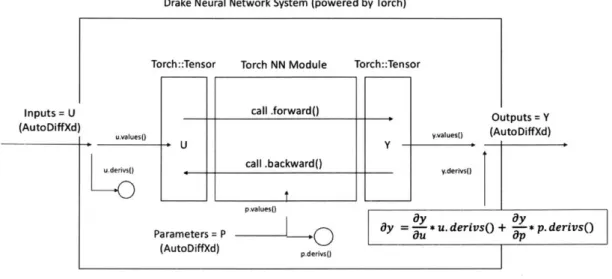
Drake Neural Network System (powered by Torch) Torch::T Inputs = U (AutoDiffXd) udU u.derivso).

ensor Torch NN Module Torch::Tens

call .forward() Y call .backward() )r Outputs = Y yalueso (AutoDiffXd) y.derivs

~|

- fL|i___ pmvalues()

Paraeter =TP * u. derivs() + *p. derivs()

(AutoDiffXd) _p.derlvso

Figure 3-1: Flow chart of the logic within NNSystem.

In the case that the type system does not need to support automatic

differentia-tion, input values are read from the NNSystem input port and loaded into a PyTorch

tensor. This tensor is used in a forward pass, producing an output PyTorch tensor.

Finally, values from the PyTorch output are packed into a Drake format for exposing

on the NNSystem output port.

When the system is asked to support automatic differentiation, input values are

taken through the same "forward pass" described above. After the PyTorch output is calculated, values from it are loaded into the value fields of a vector of AutoDiffXd's. At this point, multiple backward passes of the PyTorch neural network are initi-ated for each output of the neural network. PyTorch relies on the back-propagation algorithm to efficiently calculate gradients w.r.t. to some output throughout the net-work. We back-propagate multiple times, once for each output, (and are careful to flush gradients between every iteration) to make use of PyTorch's support of scalar differentiation.

Parameters are always stored within the PyTorch neural network object used for forward and backward passes. Additionally, they can also be exposed in a Drake Context. This doubles the storage size needed for parameters, since parameters will be stored inside the PyTorch network, and in a vector of AutoDiffXd's by Drake,

but it gives a large advantage in that it allows Drake to calculate derivatives with respect to network parameters. For example, a Drake MathematicalProgram can be constructed that takes in neural network weights as parameters. During the solving process, gradients of the output of the neural network system will be additionally taken with respect to parameters, and used to update the parameters along with whatever other decision variables are present in the program.

3.3

Custom Constraints and Costs

Drake costs and constraints can be made in much the same way. Currently, costs and constraints involving PyTorch neural networks are only supported using Drake's Python Bindings. In the case of costs and constraints, the solver will query each cost and constraint for its return value, which will be a cost in the case of Drake Costs, and a value to be compared against user-specified lower and upper bounds in the case of Drake Constraints. Because the solver does not propagate derivatives from some other computation before querying each Cost and Constraint, u.derivs() and p.derivs() in the diagram above will often be identity matrices, which can simplify the dy calculation.

dy = dy/du * du + dy/dp * dp

=

dy/du I +

dy/dp *

I

= dy/du +

dy/dp

All variables above are vector-valued. In the code, we assert that the length of derivative vectors contained within all AutoDiffXd's on the inputs and potentially the parameters are equal in length. The length of this derivative vector need not be equal to the sum of the number of inputs and network parameters. For example, taking an extreme case, if a user wanted to only expose a subset of the network parameters for automatic differentiation, they could create costs and constraints with respect to only certain weights, such as the final layer weights of a pretrained network.

In order to give constraints to the solver equation of the form ui,t = ir(xi,t) or quadratic costs of the form

Ijuj,t

- ir(xj,t)

11,

we need to define custom costs and

constraints involving PyTorch neural networks. Drake's Python bindings make this

easy. Below, we present some sample code showing how to use NNSystem logic for

easily defining an automatic diffferentiation-supported cost or constraint.

1 # Drake custom Constraint Pseudocode

2 def makecustomL2_policy-constraint(net.constructor):

3 # Constraint interface necessitates taking

4 # a flat vector of decision variables.

5 def constraint (decision-variables):

6 x, u, netparams = unpack.method(decisionvariables)

7

8 # Construct a fresh network here with net-params

9 net = netconstructor(net-params)

10

11 # Use NNSystem logic to forward pass, and possibly propagate gradients

12 if isinstance(decision-variables[O], float):

13 out = NNSystemForward_[float (x, net)

14 else:

15 out = NNSystemForard[AutoDiffXd] (x, net)

16 return 0.5*(out - u).dot(out - u)

17

18 return constraint

Test Method for NNSystem, Costs, and Constraints. Like in the case of

NNSystem, we can manually check the autodiff flow by doing finite differences at each

input of the cost/constraint and verifying that the actually output delta agrees with

what automatic differentiation tells us.

1 # Gradient Test Case Pseudocode

2 def testconstraint(constraint):

3 DELTA = le-3

4 ATOL = ie-3

5 random-floats = np.randomrand(n-inputs)

6 randomads = np.array([AutoDiffXd(val, []) for val in random-floats])

7 for i in range(n-inputs):

8 # Use AutoDiff

9 ad = constraint(random-ads)

10

11 # Use Finite Differencing

12 before = constraint(random-inputs)

13 randominputs[i] += DELTA

14 after = constraint(random-inputs)

15 random-inputs[i] -= DELTA # Undo

16 fd = (after - before) / (2 * delta)

3.4

Implementation and Evaluation

Below is the equation and matrix dimensions involved in performing derivative calcu-lation of NNSystem at its output with respect to its inputs and parameters. Up to two Jacobian matrices 1 and 2 are created internally over the course of this calculation. Though assembling these matrices completely requires more memory than a for-loop based approach, if there is sufficient memory available, it allow usage of optimized matrix multiplication kernels. Additionally, we provide a justification for construct-ing the full Jacobians based on an analysis of the unavoidable memory requirements of the parameters we do not have control over, u.derivso and p.derivs(.

dy = -- * u.derivs() + * p.derivs() (3.1)

du

dp

(out, in) (in, derivs) (out, param) (param, derivs)

Where:

in = number of neural network inputs params = number of parameters

out = number of outputs

derivs = size of derivative vector in the AutoDiffXd's

provided by the user to NNSystem.

3.4.1

Memory usage analysis

If the user is providing gradients via AutoDiffXd's, then regardless of our method, we already have memory of size O(in * derivs)

+

((param * derivs). Fully constructing

the Jacobians involving the neural network will add memory of size O(out * in) + O(out * param). So as long as the number of neural network outputs is less than

the size of the derivative vector in each AutoDiffXd, (out < derivs) then the peak

memory usage will be at most a factor of two more than the size of the derivatives given to us by the user. We believe it is reasonable to expect out < derivs because

only have a few outputs corresponding to the action dimension of the system, or

one output corresponding to the cost/constraint output. If the user wants to take

derivatives, they will likely do so with respect to the inputs, or 1 or more layers of the

network, which will all likely be greater in size than the number of outputs. Lastly,

if no gradients are needed at all, none of the above calculation takes place, and there

is no memory usage beyond that of vanilla PyTorch.

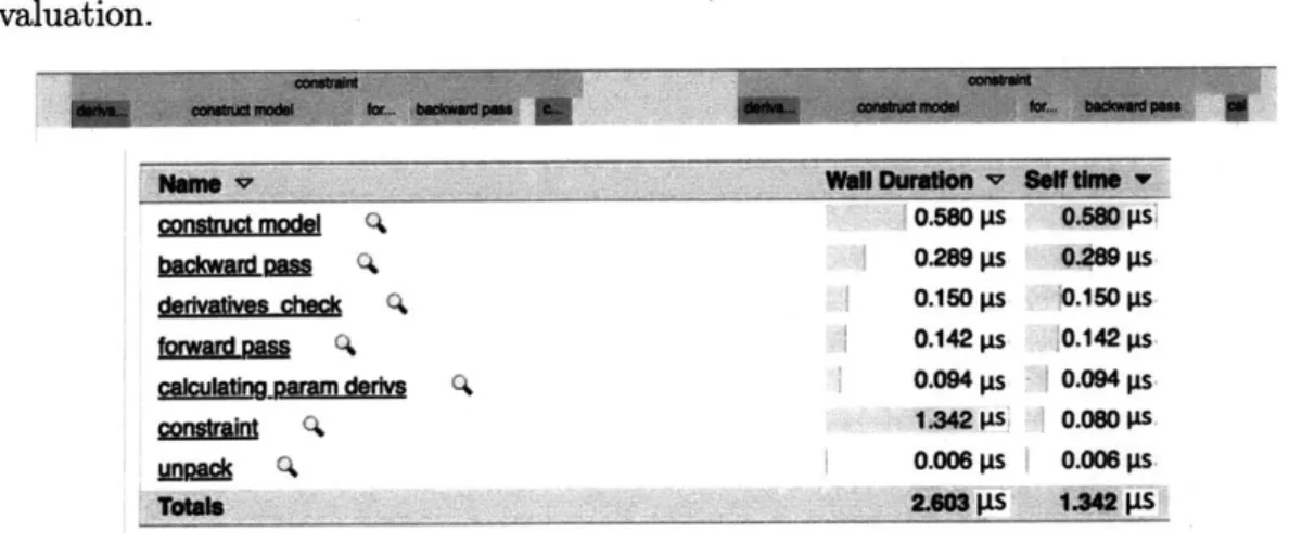
The following two figures show a timeline diagram of two constraint evaluations

during a round shared-policy trajectory optimization, and associated statistics about

the runtime. The "construct model" phase is expensive, and is needed in this case,

where model parameters are given to the optimizer and so change between each

con-straint evaluation, requiring the loading of latest weights at every round of concon-straint

evaluation.

conerm unocim 0.5801pS O.S80 PS

bai

=

m 0, 0.289 ps 0.289 Ps cdKh s chgckt g0.150 ps 10.150 ps forwCj 4 1 0.142 ps 10.142 ps calcla~g Daft cm d 0.0 94 ps 0.094 ps conait Ps PS42 0.06011s iaod c~0.006 Ps 0.006 11S Totals 2.603 9S 1.342 pS

Figure 3-2: Timeline diagram showing where time is spent in evaluating a neural network policy constraint.

Chapter 4

Understanding Simple Dynamical

Systems With Value Iteration

Because we will be focusing on convergence properties of shared-policy trajectory optimization techniques in relation to known optimal solutions, we have chosen to focus on three low-dimensional classical control tasks: the Double Integrator, Pen-dulum, and Cartpole. For these control tasks we can use Value Iteration methods to determine optimal policies, since such methods give a guarantee of convergence to the global optimal solution (barring discretization error). Having a known optimal policy will be crucial to our experiments for having a baseline to compare against, and for running experiments to inform setting hyperparameters in our methods - like determining which cost functions make for easily-learned policies and what are the minimum size networks that we should use to be able to fit those policies.

4.1

Value Iteration Background

Value Iteration, in its simplest form, is a dynamic programming algorithm which recursively solves for an optimal cost-to-go = J* over a discretized state and action

space. From a default initialization at every J*(s, a) = 0, the following update is

j*(si) += min[g(si, a) +

j*(f(si,

a))]

aEA

(4.1)

where g is the cost of being in state s and taking action a, f(s, a) is the transition

function returning the successor state of s having taken action a, and J* is the current

approximation of the optimal cost-to-go J*. We can use our approximate optimal

cost-to-go J* to derive a policy by, intuitively, choosing an action that will result in

the lowest instantaneous cost and future cost-to-go:

fr*

(s)

= arg min[g(si,

aEA

4.2

Introducing The Tasks

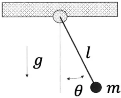
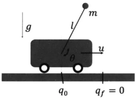
Double Integrator: A very simple

system with one degree of freedom. It

follow the following equations of motion:

4 = u,

ul

<= 1 The physical analogue of this system is a brick sliding on a

friction-less surface with a constraint on

maxi-mum torque that can be applied.

Pendulum: A simple torque lim-ited pendulum, our goal is to regulate it to the static, upright position. This may require several "pumps" to build up en-ergy to reach the upright position. Based on the strength of time and input

penal-ties, an optimal controller will prioritize

using the least force and achieving the

upright position the earliest.

a) + j*(f(s , a))]

m

(4.2)

U

qf=

0

Figure 4-1: Double Integrator System

:m

Cartpole:

A traditional Cartpole,

which has a pendulum and an

addi-tional degree of freedom in the form of

a rolling cart base. For a state vector of

(x, 9, 0, 9), the goal is to regulate the

sys-tem to (0, r, 0,0), a stationary upright

position at x

=

0. Like the pendulum

task, this may require building up energy

via pushing the cart back and forth before

1g

q0

qf=

Figure 4-3: Cartpole System

a successful swing-up can be achieved.

4.2.1

Our Desired Experiments

1. We would like to gain experience with and visually verify optimal policies for

very simple classical control tasks like the double integrator and pendulum,

where the shape of optimal policies are known.

2. We would like to make sure we can find small neural networks that can easily

fit to the Value Iteration solutions.

3. We would like to see if there is any strange behavior in our baselines due to

discretization error introduced by our value iteration process, which discretizes

the state and input spaces into bins in order to do its calculation.

4.2.2

Experiment 1: Visually Inspecting Value Iteration

Re-sults

For the double-integrator and Pendulum, we can visualize the cost-to-go and policy

found by value iteration. Below are several three dimensional visualizations of the

cost-to-go and policy solutions returned by value iteration for the double-integrator

with min-time and quadratic-cost formulations. The quantity of interest, cost-to-go

or policy action, is displayed in the z dimension, while the state space is represented

in the x and y dimensions of each graph.

Double Integrator V.I.

Cost-to-go Min-time Quadratic-cost

~4

q .10.0 12 10 8 6 4 2 0 S 1400 .4 .- 1200 f 1000 600 400 10.00 Policy M50 .25 .0 .00 4 10

a,

1 ot q_{2 5050700} -4 .~

~J1.00

4

0.75 0.50 .50 1.00

~

3 10075 qdot -10.0 00 2 q 505 -q . ,100 0 4

Figure 4-4: Value Iteration vs. Trajectory Optimization Results for Double Integrator

There are a few key observations here. The first is that the min-time policy has a roughly parabolic switching surface, which agrees with literature online for this prob-lem formulation 113]. The second is that the policy in this simple system changes very abruptly, due to "bang-bang" control being optimal. Finally, we note how drastically the cost-to-go changes between the min-time and quadratic-cost formulations of the problem. Because the cost-to-go is calculated by repeatedly adding the optimal in-stantaneous cost along a trajectory via equation 4.2, it makes sense that visually small differences in a policy could accumulate to create large differences in the cost-to-go.

Below are the cost-to-go and policy returned by value iteration for the pendulum swing-up task. In both rows, we visualize a quadratic-cost formulation. However, the top row has a quadratic cost term with a coefficient twenty-five times smaller than on the bottom row. Because the input limit is rather low (5N -m in this case), the policy on the upper row saturates the input limits and leads to a very sharp, discontinuous

policy. Note: the visualization technique forms a surface over a mesh of z axis values

on an x-y grid, so the policy will always seem continuous in our visualization, even if in reality, the optimal policy is not continuous (like in the case of bang-bang control for the double-integrator).

Pendulum V.I.

Cost-to-go Policy so 2 So g(x, u) -2 =2x x+u u 20 Jul < 5 1 25 et- 5 1., 3 4-7.5 q 0 -0.0 2550 i100 250 200- 2 I.150 0 g(x, u) 100 -2 2x X + 25U 50

Jul < 5

ALI

~

21ot 01 2 3 7.,54f 0 1 2 3 6 Uteta 4 6 1-0. 0 q !

Figure 4-5: Value Iteration vs. Trajectory Optimization Results for Pendulum

4.2.3

Experiment 2, Evaluating Minimum Neural Network Sizes

for Fitting Value Iteration Policies

Now that we've found some optimal policies from value iteration, we'd like to see

what minimally-sized neural networks can be used to fit those policies. When we

eventually perform shared-policy trajectory optimization in Chapters 5 and 6, these

findings will guide our network selection. We test four network sizes, all of which

have a standard feed-forward architecture with one or two hidden layers of size 8

or 32. Activations are all chosen to be ReLU. Each column represents a particular task+objective formulation: in this case, the min-time and quadratic cost Double Integrator policies, and the low quadratic cost and high quadratic cost Pendulum policies.

The network size chosen as residing at a good sweet spot between complexity and ability to fit the optimal solution has been bolded in each column.

Each cell contains a tuple of

(Avg L2 Error fitting VI cost-to-go, Avg L2 Error fitting the VI policy).

network DI min-time DI quad.-cost Pend low u-cost Pend high u-cost 1 layer, sz 8 0.436, 0.061 1600, 0.006 0.2, 0.017 14.5, 0.004 1 layer, sz 32 0.025, 0.015 1600, 0.005 0.058, 0.006 0.45, 0.002

2 layer, sz 8

0.016, 0.002 49, 0.001

0.021, 0.003

0.3, 0.001

2 layer, sz 32 0.001, 0.001

17, 0.001

0.012, 0.003

0.05, <0.001

Table 4.1: Minimal Neural Network Testing to Fit Optimal Policies from Value Iteration

4.3

Trajectory Optimization and Direct Collocation

Having gained some intuition with value iteration and done some experimentation with minimal neural network sizes to fit them, we now turn our attention to a dis-tinct, third topic, trajectory optimization. Trajectory optimization is a powerful class of algorithms in which we seek to find an optimal sequence of controls for some system given a cost function, equality and inequality constraints, and an initial state. This is accomplished by setting up an optimization problem where we dicretize the tra-jectory in time to a series of knot points (Xt, Ut) which describe the state and action, respectively, at a time t. We seek to minimize the total cost at these knot points, subject to constraints that consecutive knot points obey dynamics constraints of the system. We can also easily apply other constraints specifying things like input and state-space limits. The process of converting a continuous optimal control problem into a non-linear programming problem knot points is called transcription.

4.3.1

Direct Transcription and Direct Collocation

The equation below describes the general format of a transcripted trajectory opti-mization problem, in its collocation (as opposed to shooting) form.

N-1

min E g(x,,un)dt

X~ .. Xi~ .UN-1 n=O

(4.3)

Xn+1= x-n + f (Xn, un)dt, Vn E [0,

N

- 1].

A property of collocated formulations is that they are over-specified. All states and actions are exposed for simultaneous optimization, even though an initial state and just the control sequence would be enough to fully define the trajectory. The benefit of over-specifying and exposing both states and controls as decision variables is that cost and constraints all along the trajectory can be optimized at once. Otherwise, the trajectory would be very sensitive to perturbations in the early knot points, and the method would expose less parallelism to a solver.

There are many ways to choose time intervals of knot points, and varying degrees of approximations of the dynamics we can use in our constraints between knot points. A very simple way that we could approximate our system's dynamics between knot points would be to use a piece-wise constant input trajectory and a piece-wise linear state trajectory. This choice is the one employed by the Direct Transcription method.

Another choice that strikes a potentially better balance between approximating the dynamics, producing smooth x-trajectories, and not incurring too many evalua-tions of the system is called Direct Collocation. Direct Collocation employs a piece-wise cubic polynomial to represent the state trajectory and a piece-piece-wise linear input trajectory. The dynamics constraints are enforced by adding "collocation" points at the midpoints of all segments between knots.

4.4

Experiments relating Trajectory Optimization and

Value Iteration

In order to relate solutions found via trajectory optimization methods, and known global solutions determined through Value Iteration, we perform the following two experiments:

1) We would like to find cost functions that enable us to easily perform Trajectory Optimization and Value Iteration to solve the control tasks. Having both Trajectory Optimization and Value Iteration solutions for each problem will be critical when doing comparisons between the two.

2) Once we have found policies that are seemingly optimal from Value Iteration, we would like to see how good of an estimator Trajectory Optimization, and in particular Direct Collocation is of the optimal cost-to-go and policy found from Value Iteration. Trajectory optimization introduces error via approximating the dynamics between knot points. It also is a non-convex optimization and so can get caught in local minima. Local minima, here, would indicate that the trajectory found is sub-optimal, so there is another trajectory that would satisfy the constraints of the problem but return lower cost. Therefore, ignoring error from approximation of the dynamics between knots, we would expect that the sum of costs over trajectory optimization solutions would upper-bound the optimal cost-to-go from a given initial condition. Note: Though we previously did an experiment with neural network sizing, we are now (temporarily) setting neural networks aside to just study the relationship between Value Iteration an Trajectory Optimization solutions on our simple control task and systems. We will eventually combine all components in Chapters 5 and 6.

4.4.1

Comparing Cost-to-Go and Policy Obtained from Value

Iteration and Trajectory Optimization

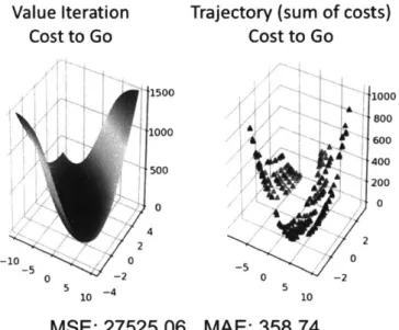
Below are visual comparisons and statistics relating the cost-to-go and policy

de-termined by Value Iteration and Trajectory Optimization, for the two visualizable,

Double Integrator and Pendulum swing-up control tasks.

Value Iteration

Cost to Go

S 1500 -1000 -50 0 4 2 -10 0 -5 0 z -2 510 -4

MSE: 27525.06

Trajectory (sum of costs)

Cost to Go

1000

800

A600

400 200 0 2 0 -2 5 10

MAE: 358.74

Figure 4-6: Double Integrator Cost to Go Comparison

Observations on the Double Integrator Task (cost-to-go):

1. Though the cost-to-go mean-squared and mean-absolute error numbers appear

high (pictured below), the trajectory optimization results do recreate the shape of the value iteration solution well, with minimal fluctuations. We believe the difference in cost-to-go at the perimeter of the inspected state space is due to the accumulation of discretization error.

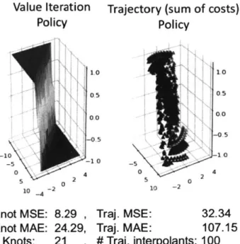
Value Iteration

Trajectory (sum of costs)

Policy

Policy

-10 5 -5 2 10 - -2

Knot MSE: 8.29

Knot MAE: 24.29,

# Knots:

21

1.0 0.5 0.0 -05 -10 1.0 0.0 -0.5 1.0 -5 10 -2 o

Traj. MSE:

32.34

Traj. MAE:

107.15

# Traj. interpolants: 100

Figure 4-7: Double Integrator Policy Comparison

Two categories of quantities are reported here: mean-squared and -absolute errors at knot points (21 for each trajectory) w.r.t. the value iteration policy, and mean-squared and -absolute errors of 100 interpolated points equally spaced in time along each trajectory w.r.t. the value iteration policy. This is valid due to Direct Collocation producing a piece-wise linear action trajectory and a piece-wise cubic state trajectory.

Observations on the Double Integrator Task (policy):

1. The results suggest that error is greater at interpolated points along a trajectory

rather than at knot points. We use this conclusion to only use knot points and not interpolants in our shared-policy trajectory optimization experiments. 2. The policy shows very good agreement between Value Iteration and Trajectory

Optimization solutions. Though the switching surface is a bit steeper in the Value Iteration solution.

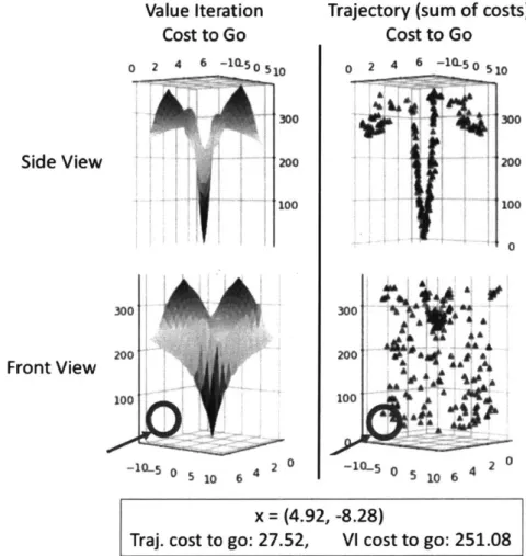
Value Iteration

Cost to Go

0 2 4 6 -1(150510 21 10

0

I0 200

100

-1-5 0 5 10 6 4 2 0

Trajectory (sum of costs)

Cost to Go

0

2 4 6 -1-50 _{5 10} 200 10() 0 300' 200 AM 100 -10-S 0 5 10 6 4 2 0 x

= (4.92, -8.28)

Traj. cost to go: 27.52,

VI cost to go: 251.08

Figure 4-8: Pendulum Cost-to-Go Comparison

Observations on the Pendulum Task:

1. In the upper diagram, we show two angles of the cost-to-go, calculated from

value iteration and from summing the costs of knot points from repeated ap-plications of trajectory optimization and attributing them to the chosen initial state.

2. In the pendulum swing-up task, there is good agreement between the two meth-ods for determining cost-to-go from one angle, but from the angle facing the plane 0 = -4, we can see that there is a large discrepancy between the results

from our usage of the methods, highlighted with a red circle. An example co-ordinate, (4.92, -8.28) is an example of a state where the pendulum is rapidly

approaching the upright position, that exhibits this discrepancy highly.

Side View

After performing further investigation, we found that this discrepancy was a result of different time-step settings between our usages of the two methods. In our Value Iteration experiment, we used a time-step of 0.0001, to have high accuracy. But in trajectory optimization, with only 20-40 knot points and a total trajectory time length of around a second for many initial conditions, it's not possible to get such high granularity over time. Along the

0

=

-0

line, time to the upright position is very short, and the "braking" force applied to the pendulum is high. The Value Iteration solution, with its small timestep, correctly calculates the high cost along this trajectory, while the trajectory optimization solution with it's large time steps, does not.

3. Once again, the average error at interpolation points along the trajectory was found to be greater than the cost at specific knot points.

4.4.2

Effect of Warm Starting on the Divergence of

Trajec-tory Optimization vs. Value Iteration Costs-to-Go and

Policies

In the first two rows of the following three diagrams, we will explore the distribution of differences in cost-to-go and the policy as reported by Value Iteration and Trajectory Optimization, for the Double Integrator, Pendulum, and Cartpole tasks. In the final row of each diagram, we plot the difference in policy vs the difference in cost-to-go between the two methods, on each axis, to look for noteworthy correlations. In each column of the three diagrams, we set the warm starting scheme for Trajectory Opti-mization to be either 1) None -zero-initializing the state and input decision variables, 2) Linear - initializing the state decision variables with a linear interpolation between the initial state and the desired goal state, or 3) Random - randomly initializing the state with values drawn from a uniform distribution over the state boundaries used in Value Iteration, for each state dimension.

Observations on the Double Integrator Task:

Warm Start

DOUBLE INTEGRATOR = None

Av: 45 ICIt-I--SI: 30 Acost-to-go MSE: 5.605 histogram MAE: 45 -150 -100 -50 0 50 Warm Start = Linear Warm Start = Random Avg: -49 Avg: -49 Std: 38 Sd: 37

MSE: 6.7e5 MSE: S.9e5

MAE: 50 MAE: 50 -150100 -50 0 50 150 -100 -50 0 50 Apolicy histogram -.6 -.4 -.2 0 .2 .4 .6 Apolicy VS. Acost-to-go Avg: -0.01 Sti: 0.14 MSE: 3.7 MAE: 0.06 .6 .2 -.4 -.6 -200 40 -100 -50 0 50 Acost-to-go 4d Avg: -0.01 St: 0.15 MSE: 3.64 MAE: 0.06 -.6 -A -.2 0 2 A .6 .6 0 .. ... -.2 -A -200 -150 -100 -50 0 50 cost-to-g0 Avg: -0.01 5W: 0.19 MSE: 5.87 MAE: 0.08 -.6 -.4 -.2 0 .2 4 .6 .6 0--.4 -.6 -200 -150 -100 -50 0 50 Acost-to-go

Figure 4-9: Cost-to-go vs. Policy Discrepancies for Double Integrator

1. Linear warm starting appears to be the best choice for minimizing Acost-to-go

= A J = Jtra., - JvI.

2. All policies seem to be very accurate, with no noticeable deviations between the

two methods.

3. Because of the accuracy of the policy vs the cost-to-go, the lowest row of plots all report back simple linear relationships, with just a few outliers.