HAL Id: inria-00515531
https://hal.inria.fr/inria-00515531
Submitted on 7 Sep 2010
HAL is a multi-disciplinary open access
archive for the deposit and dissemination of sci-entific research documents, whether they are pub-lished or not. The documents may come from teaching and research institutions in France or abroad, or from public or private research centers.
L’archive ouverte pluridisciplinaire HAL, est destinée au dépôt et à la diffusion de documents scientifiques de niveau recherche, publiés ou non, émanant des établissements d’enseignement et de recherche français ou étrangers, des laboratoires publics ou privés.
Adaptive geometry compression based on 4-point
interpolatory subdivision schemes with labels
Hui Zhang, Jun-Hai Yong, Jean-Claude Paul
To cite this version:
Hui Zhang, Jun-Hai Yong, Jean-Claude Paul. Adaptive geometry compression based on 4-point in-terpolatory subdivision schemes with labels. International Journal of Computer Mathematics, Taylor & Francis, 2007, 16p. �inria-00515531�
Adaptive geometry compression based on 4-point interpolatory subdivision schemes with labels Hui Zhang∗†, Jun-Hai Yong† and Jean-Claude Paul† ‡
†School of Software, Tsinghua University, Beijing 100084, P. R. China ‡CNRS, France
(Received 00 Month 200x; In final form 00 Month 200x)
We propose an adaptive geometry compression method with labels based on 4-point interpolatory subdivision schemes. It can work on digital curves of arbitrary dimensions. With the geometry compression method, a digital curve is adaptively compressed into several segments with different compression levels. Each segment is a 4-point subdivision curve with a subdivision step. Labels are recorded in data compression to facilitate merging those segments in data decompression. In the meantime, we provide high-speed 4-point interpolatory subdivision curve generation methods for efficiently decompressing the compressed data. For an arbitrary positive integer k, formulae of the number of the resultant control points of a 4-point subdivision curve after k subdivision steps are provided. Some formulae for calculating points at the kth subdivision step are presented as well. The time complexity of the new approaches is O(n), where n is the number of the points in the given digital curve. Examples are provided as well to illustrate the efficiency of the proposed approaches.
Keywords: Geometry compression; Subdivision scheme; 4-point subdivision; Interpolatory
subdivision; High-speed curve generation
AMS Subject Classification: 68P30; 94B27
1 Introduction
It is a common practice to compress data before they are archived. With ubiq-uitous applications of computers and network, gigantic amount of data are continuously generated. In the meantime, the increasing demand for commu-nication and data exchange over network beats the limitation of the network band. Data compression becomes more and more important and receives more and more attentions [7, et al]. While data compression has a long history and has achieved a high level of sophistication, some new tools are eager to
be discovered to fill the gap between the requirement and the ability of data compression. Geometry compression is relatively new, and becomes a hot topic in a short time after it appeared [6,7,9–12,14, et al]. Wavelet transforms [7, et al], multiresolution [6, et al] and various trees [14, et al] are frequently used in geometry compression.
Almost all geometry compression methods focus on how to compress three-dimensional meshes. In this paper and [13], we propose new geometry com-pression methods based on 4-point interpolatory subdivision schemes. With our new methods, a digital curve of an arbitrary dimension is compressed into one or several subdivision curve segments. The advantages of our methods are at least as follows.
• It is able to work on a digital curve of arbitrary dimensions. And any
se-quence of data can be considered as a digital curve of certain dimensions.
• The set of the inner control points of the resultant subdivision curves is
exactly a subset of the points of the compressed curve.
• It is possible to simplify the pattern recognition of some digital curves into
the pattern recognition of the subdivision curve segments after data com-pression. The inner control points of the resultant subdivision curves may be considered as the key points of the given digital curves, since they can be used to reproduce the given digital curves after data decompression. Our work of this paper and [13] gives contributions to the area about subdi-vision curves and surfaces as well. The first subdisubdi-vision scheme for generating subdivision curves was proposed by Chaikin [2] in 1974. The 4-point inter-polatory subdivision [4] appeared in 1987. Recently, research on subdivision schemes for generating curves and surfaces becomes popular in graphical mod-eling [3,9, et al], animation [15, et al] and CAD/CAM [8, et al] because of their stability in numerical computation and simplicity in coding. Much work on subdivision surfaces is carried out in several important topics such as Boolean operations [1], mesh editing [15], and adaptive tessellation [9]. And a lot of work [5, et al] has been carried out on the 4-point subdivision schemes as well. In this paper and [13], we provide approaches for the high-speed 4-point in-terpolatory subdivision curve generation to speed up the data decompression. [13] is presented at IWICPAS (the International Workshop on Intelligent Computing in Pattern Analysis/Synthesis). Some further work based on [13] is carried out in this paper. For data compression, the geometry compression methods are replaced by the new ones with labels in this paper. In the new geometry compression methods, on the one hand, labels are used to identify the open case and the close case. On the other hand, we use labels to facilitate the merging process in data decompression, i.e., labels are used to identify the segments which should be merged during the data decompression. For data decompression, some more formulae for calculating the control points at the
kth subdivision step with respect to the original control points are provided.
With the new formulae, the relationship between the control points at the kth subdivision step and the original control points may become more clear.
The remaining part of the paper is arranged as follows. A brief review of the 4-point interpolatory subdivision curve is given in Section 2. Data compres-sion methods with labels are provided in Section 3. The high-speed generation approaches are provided in Section 4 for the open 4-point interpolatory sub-division curve and the closed 4-point interpolatory subsub-division curve, respec-tively, to speed up the data decompression. Section 5 uses some examples to illustrate the efficiency of the proposed approaches. Some concluding remarks are given in the last section.
2 4-Point Interpolatory Subdivision Schemes
In this section, we briefly go through the 4-point interpolatory subdivision schemes given by [4]. Initially, a set of points M0 = {P0,0, P1,0, · · · , Pn0−1,0}
is given, where Pi,0(i = 0, 1, · · · , n0− 1) are points, and n0 is the number of the points. The subdivision is preformed in a recursive procedure. At each subdivision step, some points before the subdivision are inherited, and some new points are inserted into the point set such that the number of the points usually becomes larger and larger. Let Mk = {P0,k, P1,k, · · · , Pnk−1,k} be the
resultant point set after the kth (k = 0, 1, 2, · · ·) subdivision step, where nk is the number of the points in Mk. All points Pi,k in Mk are called control
points as well.
The 4-point interpolatory subdivision curves can be classified into categories: the open case or the close case. At the kth subdivision step, the points inherited from Mk−1 are Pi,k−1, where i = 1, 2, · · · , (nk−1 − 2) for the open case, and
i = 0, 1, · · · , (nk−1−1) for the close case. The point Pj,k to be inserted between
Pi,k−1 and Pi+1,k−1 at the kth subdivision step is
Pj,k = (w + 0.5)(Pi,k−1+ Pi+1,k−1) − w(Pi−1,k−1+ Pi+2,k−1), (1) for each i = 1, 2, · · · , (nk−1− 3) under the open case, and
Pj,k = (w + 0.5)(P(i%nk−1),k−1+ P((i+1)%nk−1),k−1)
−w(P((i−1)%nk−1),k−1+ P((i+2)%nk−1),k−1), (2)
for each i = 0, 1, · · · , (nk−1− 1) under the close case, where the weight w is a
given real number. Usually, the value of w is suggested to be 1
16. In Equation
(2), the modulus symbol (%) is used such that each subscription is in the set {0, 1, · · · , nk−1− 1}. Note that from Mk−1 to Mk, the points P0,k−1 and
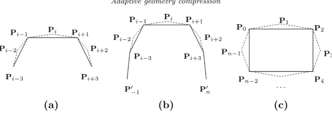
Pi−3 Pi−2 Pi−1 Pi Pi+1 Pi+2 Pi+3 P0 −1 Pi−3 Pi−2 Pi−1 Pi Pi+1 Pi+2 Pi+3 P0 n P0 P1 P2 P3 P4 · · · Pn−2 Pn−1 (a) (b) (c)
Figure 1. Principle of geometry compression: (a) mask of a removable point, (b) boundary case, and (c) close case.
Pnk−1−1,k−1 are discarded for the open case after the subdivision, which is
called the shrink property of an open 4-point interpolatory subdivision curve. When k → ∞, the point set M∞ becomes a limit subdivision curve. M∞ is
an open curve under the open case, and a closed curve under the close case.
3 Data Compression
In this section, we propose geometry compression methods with labels for digital curves based on the above schemes. Here, a digital curve is an open polygonal curve or a closed polygonal curve (i.e. a polygon). Thus, we need the label Lopenhere to identify the open polygonal curve, and the label Lclose
to identify the closed polygonal curve. In either case, the digital curve is rep-resented by n vertices {P0, P1, · · · , Pn−1} with a label Lopen or Lclose. The principle of the geometry compression is, as shown in Figure 1(a),
• that for the open case, we do not need to store Pi which satisfy
kPi− [(w + 0.5)(Pi−1+ Pi+1) − w(Pi−3+ Pi+3)]k2≤ e, (3) where i = 3, 4, · · · , (n − 4), and e is the given error tolerance;
• and that for the close case, we do not need to store Pi which satisfy
° °Pi−
£
(w + 0.5)(P(i−1)%n+ P(i+1)%n) − w(P(i−3)%n+ P(i+3)%n)¤°°2 ≤ e,
(4) where i = 1, 3, 5, · · ·, i ≤ (n − 1), and e is the given error tolerance.
The points satisfying Equations (3) and (4) are called the removable points, which can be reproduced by the 4-point interpolatory subdivision schemes.
If the given digital curve is a closed curve with an even number of the vertices and each odd vertex Pi, where i = 1, 3, · · · , (n − 1), is a removable
point, the digital curve can be compressed into a closed subdivision curve with the control points {P0, P2, · · · , Pn−2}. Thus, the compression ratio is 2 : 1.
And the procedure can be recursively carried out, so the compression ratio can be higher than 2 : 1. Otherwise, we compress the digital curve in the same way as the open case.
If the given digital curve is an open curve and {Pa, Pa+2, · · · , Pb} are
remov-able points, then the points {Pa−3, Pa−2, · · · , Pb+2, Pb+3} can be compressed
into {P0
−1Pa−3, Pa−1, · · · , Pb+1, Pb+3, P0n}, where
P0−1 = (w + 0.5)(Pa−3+ Pa−1) − Pa−2
w − Pa+1 (5)
and
P0n= (w + 0.5)(Pb+3+ Pb+1) − Pb+2
w − Pb−1 (6)
are two auxiliary points. Because of the shrink property, we need two auxiliary points P0
−1 and P0n to keep Pa−3 and Pb+3 after one subdivision step. Under
this case, the compression ratio is [(b − a) + 7] : (b−a)+122 . For example, as shown in Figure 1(b), when a = b = i, the compression ratio is 7 : 6.
After some removable points are removed, the digital curve becomes a subdi-vision curve segment or several subdisubdi-vision curve segments. Each subdisubdi-vision curve segment can be recursively compressed. Thus, a subdivision curve seg-ment may be compressed into several subdivision curve segseg-ments again. In the inverse process, those subdivision curve segments should be decompressed and then merged together into the segment, on which the decompression process will be carried out again to recover the removable control points. In this paper, we use labels to identify the subdivision curve segments, which are from the same subdivision curve segment. Thus, the labels will facilitate the decom-pression process in coding. As shown in the following algorithms, the label
Lmerge(k) is used to identify the subdivision curve segments, which should be
decompressed and merged together into a segment at the data decompression process. Here, the value of k in the label Lmerge(k) will be used at the data decompression process. After merging the segments into a whole segment, k subdivision steps will be carried out on the whole segment at the data decom-pression process. For example, in the following algorithms, one branch will lead to a compressed data set {Lmerge(k), S1, S2}. To decompress the data set, we
need to decompress S1 and S2 first. And then, merge the two decompressed
point sets into a control point set of a subdivision curve segment. k subdivi-sion steps will be carried out on the subdivisubdivi-sion curve segment to obtain the resultant decompressed data. And the label Lsingle(k) is used to identify the
subdivision steps at the data decompression process.
Algorithm 1. Geometry compression with labels for the open case.
Input: the point set {P0, P1, · · · , Pn−1}, the error tolerance e, the
weight w, and the current subdivision step k (with an initial value k = 0).
Output: a set of compressed data set S (with an empty initial value S = Φ).
1 if (n ≤ 7) // note: the number of the vertices is too small for the compression. begin
let M be a subdivision curve with {P0, P1, · · · , Pn−1}, the subdivision
step k and the label Lopen;
let S = {Lsingle(0), M}; output S; go to Step 7; end 2 let a = 0; for (i = 3; i ≤ (n − 4); i+ = 2) begin
if (Pi is a removable point according to Equation (3) )
begin
let a = i; go to Step 3; end
end
3 if (a is zero) // note: no points could be compressed. begin
let M be a subdivision curve with {P0, P1, · · · , Pn−1}, the subdivision
step k and the label Lopen; let S = {Lsingle(0), M};
output S; go to Step 7; end
else if (a > 3) // note: the data will be compressed into several segments. begin
let M1 be a subdivision curve with {P0, P1, · · · , Pa−3}, the
subdivi-sion step 0 and the label Lopen;
end 4 let b = a;
for (i = a + 2; i ≤ (n − 4); i+ = 2) begin
if (Pi is not a removable point according to Equation (3) ) go to Step 5; else let b = i; end 5 if ( b < (n − 4) ) begin
call Algorithm 1 with the input
{P0
−1Pa−3, Pa−1, · · · , Pb+1, Pb+3, P0n}, e, w and 1, where P0−1
and P0
nare calculated according to Equations (5) and (6), and obtain
the set S1;
call Algorithm 1 with the input {Pb+3, Pb+4, · · · , Pn−1}, e, w and 0,
and obtain the set S2;
if (a > 3) let S = {Lmerge(k), M1, S1, S2}; else let S = {Lmerge(k), S1, S2}; end else begin if (a > 3) begin
call Algorithm 1 with the input
{P0
−1Pa−3, Pa−1, · · · , Pb+1, Pb+3, P0n}, e, w and 1, where
P0
−1 and P0n are calculated according to Equations (5) and (6),
and obtain the set S1;
let S = {Lmerge(k), M1, S1};
end else begin
call Algorithm 1 with the input
{P0
−1Pa−3, Pa−1, · · · , Pb+1, Pb+3, P0n}, e, w and (k + 1),
where P0
−1 and P0n are calculated according to Equations (5)
and (6), and obtain the set S; end
end 6 output S;
Algorithm 2. Geometry compression with labels for the close case. Input: the point set {P0, P1, · · · , Pn−1}, the error tolerance e, the
weight w, and the current subdivision step k (with an initial value k = 0).
Output: a set of compressed data set S (with an empty initial value S = Φ).
1 if (n < 6) // note: the number of the vertices is too small for the compression. begin
let M be a subdivision curve with {P0, P1, · · · , Pn−1}, the subdivision
step k and the label Lclose;
Let S = {Lsingle(0), M}; go to Step 4;
end
2 if ( n is odd) begin
call Algorithm 1 with the input {P0, P1, · · · , Pn−1}, e, w and k, and
obtain the set S;
let S have the label Lclose; go to Step 4;
end
3 if ( all points Pi (where i = 1, 3, · · · , (n − 1)) are removable points)
begin
call Algorithm 2 with the input {P0, P2, · · · , Pn−2}, e, w and (k + 1),
and obtain the set S; end
else begin
call Algorithm 1 with the input {P0, P1, · · · , Pn−1}, e, w and k, and
obtain the set S;
let S have the label Lclose;
end 4 output S;
5 End of Algorithm 2.
In Algorithms 1 and 2, we only check whether the points in the given point set are removable points at most twice, and we do not check whether any aux-iliary point produced by Equation (5) or (6) is a removable point. Therefore, although Algorithms 1 and 2 contain loops and recursive procedures, the time complexity of both Algorithms 1 and 2 is O(n).
4 Data Decompression
With the method introduced in Section 3, a digital curve is compressed into one or some subdivision curve segments. Hence, the problem here is how to obtain the points in Mk, which is the point set after k subdivision steps are
carried out from the initial control point set M0. According to the method in Section 2, in order to obtain Mk, we need to calculate all the control points
in M1, M2, · · · , Mk−1. Unfortunately, we do not need M1, M2, · · · , Mk−1 at
all, but only Mk. Thus, we need extra memory to store those unnecessary
points, and experience shows that the time cost in this way increases sharply with respect to the subdivision step k. In this section, we will provide the high-speed generation approaches. One is for the open subdivision curve, and the other one is for the closed curve.
4.1 Open curve generation
In this subsection, we only consider the open 4-point subdivision curve. First, we need to obtain the value of nk, which is the number of points in Mk, such that we could allocate memory to store the coordinates of the points in Mk
before computing the coordinates. According to Section 2, from Mk−1 to Mk, all the points except for the first and the last points in Mk−1 are inherited,
and the number of new points inserted into Mk is 3 less than the number of
the points in Mk−1. Thus, we obtain nk with respect to nk−1 in Lemma 4.1. Lemma 4.1 If n0 ≥ 5, the number of the points in Mk is nk= (nk−1− 2) +
(nk−1− 3) = 2nk−1− 5, for k = 1, 2, · · ·.
According to Algorithms 1 and 2, no subdivision is necessary to be performed on a set of points which number is less than 5. Therefore, we do not consider the case when n0 < 5. Recursively apply the above lemma, and we obtain nk
with respect to n0 in Theorem 4.2.
Theorem 4.2 If n0≥ 5, the number of the points in Mkis nk= 2k(n0−5)+5,
for k = 1, 2, · · ·.
The remaining part of the subsection will provide the method for calculating the coordinates of the points in Mk. It is based on the following important
theorem. The theorem can be proved by the mathematical induction method according to Section 2.
Theorem 4.3 For k = 0, 1, 2, · · ·, we have
1. Pi×2k+2,k = Pi+2,0, where i = 0, 1, 2, · · ·, and i × 2k+ 2 < nk. 2. P(2k)×i+3,k
= w(−2(−k)h+2kwk(4w−1)hh+dk(1−4w)−ek(1−4w))Pi,0
+−(dk(1+h−4w−4hw)+ek(h−1+4w−4hw)+8×24(4w−1)h kw(k+1)h−2(1−k)h)Pi+1,0
+−(−2h+dkh+dk−4d2hkw+ekh−ek+4ekw)Pi+2,0
+8×2kw(k+1)h+dk(4hw−1−h+4w)+e4(4w−1)hk(1−h−4w+4hw)−2(1−k)hPi+3,0
+−w(2kwkh−2(−k)(4w−1)hh−4ekw+ek+4dkw−dk)Pi+4,0 ,
where w ∈ ¡0,161¢, d = 1+√1−16w4 , e = 1−√1−16w4 , h = √1 − 16w, i = 0, 1, 2, · · ·, and i + 4 < n0. 3. P(2k)×i+3,k = ³ 1 12×2k −12×81 k −8×4kk ´ Pi,0 + ³ − 2 3×2k + 6×81k +2×41k +2×4kk ´ Pi+1,0 +¡1 −41k − 4(k+1)3k ¢ Pi+2,0 + ³ 2 3×2k −6×81k + 2×4kk +2×41k ´ Pi+3,0 + ³ − 1 12×2k +12×81 k −8×4kk ´ Pi+4,0 , where w = 161, i = 0, 1, 2, · · ·, and i + 4 < n0. 4. P(2k)×i+1,k = −w(−2(−k)h+2kw(4w−1)hkh+dk(4w−1)+ek(1−4w))Pi,0 +−(ek(h−1+4w−4wh)+dk(1+h−4w−4wh)−8×24(4w−1)h kw(k+1)h+2(1−k)h)Pi+1,0 +−(dk(h+1−4w)+e2hk(h−1+4w)−2h)Pi+2,0 +−(ek(h−1+4w−4wh)+dk(1+h−4w−4wh)+8×24(4w−1)h kw(k+1)h−2(1−k)h)Pi+3,0 +w(−2(−k)h+2kwk(4w−1)hh+dk(1−4w)+ek(4w−1))Pi+4,0 , where w ∈ ¡0,161¢, d = 1+√1−16w4 , e = 1−√1−16w4 , h = √1 − 16w, i = 0, 1, 2, · · ·, and i + 4 < n0. 5. P(2k)×i+1,k = ³ −1 12×2k +12×81 k −8×4kk ´ Pi,0 + ³ 2 3×2k −6×81k + 2×4kk +2×41k ´ Pi+1,0 +¡1 − 3k 4(k+1) −41k ¢ Pi+2,0 + ³ − 2 3×2k + 6×81k +2×4kk +2×41 k ´ Pi+3,0 + ³ 1 12×2k −12×81 k −8×4kk ´ Pi+4,0 , where w = 161, i = 0, 1, 2, · · ·, and i + 4 < n0.
algorithm for calculating the coordinates of the points in Mk.
Algorithm 3. Calculating coordinates of points in Mk for the open case. Input: M0 and the weight w with the assumption that n0≥ 5.
Output: Mk.
1 calculate nk according to Theorem 4.2;
2 allocate memory for Mk to store the coordinates of nk points in Mk; 3 for (i = 0, i0 = 2, ik = 2; ik< nk; i + +, i0+ +, ik+ = 2k) Pik,k = Pi0,0 according to Theorem 4.3; 4 P0,k = P0,0; P1,k = P1,0; Pnk−1,k = Pn0−1,0; Pnk−2,k = Pn0−2,0; 5 for (i = k; i >= 1; i − −) begin P = (w + 0.5)(P1,k+ P2,k) − w(P0,k+ P2i+2,k); P2i−1+2,k = (w + 0.5)(P2,k+ P2i+2,k) − w(P1,k+ P2i+1+2,k); P0,k = P1,k; P1,k = P; for (j = 2i+ 2i−1+ 2, m = 2; j < n k− 3 − 2i−1; j+ = 2i, m+ = 2i) begin Pj,k = (w + 0.5)(P2i+m,k+ P2i+1+m,k) − w(Pm,k+ P3×2i+m,k); end P = (w + 0.5)(Pnk−2,k+ Pnk−3,k) − w(Pnk−1,k+ Pnk−3−2i,k); Pnk−3−2i−1,k = (w + 0.5)(Pn k−3,k + Pnk−3−2i,k) − w(Pnk−2,k + Pnk−3−2i+1,k); Pnk−1,k = Pnk−2,k; Pnk−2,k = P; end 6 End of Algorithm 3.
In Algorithm 3, we assume that n0≥ 5, so we have nk≥ 5. In the algorithm,
any point in Mk, except for P0,k, P1,k, Pnk−1,k and Pnk−2,k, are calculated only once. Therefore, the time complexity of Algorithm 3 is O(nk), which is
the lowest bound of calculating all points in Mk. 4.2 Closed curve generation
This subsection focuses on the approach for the high-speed generation of the closed subdivision curve. According to Section 2, from Mk−1 to Mk, all the
points in Mk−1 are inherited, and the number of new points inserted into Mk is equal to nk−1. Thus, we obtain the conclusions in Lemma 4.4 and Theorem
4.5.
Lemma 4.4 The number of the points in Mk is nk= 2nk−1, for k = 1, 2, · · ·.
Theorem 4.5 The number of the points in Mk is nk = n0 × 2k, for k =
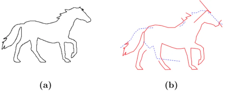
(a) (b)
Figure 2. Example 1: (a) before data compression, and (b) after data compression. To calculate the coordinates of the points in Mk, one important conclusion
is drawn in Theorem 4.6.
Theorem 4.6 For k = 0, 1, 2, · · ·, we have Pi×2k,k = Pi,0, where i =
0, 1, 2, · · ·, and i × 2k< n k.
Thus, according to Theorem 4.6 and Equation (2) in Section 2 for calculating new points, we obtain the following algorithm. Similar to Algorithm 3, the time complexity of the following algorithm is O(nk).
Algorithm 4. Calculating coordinates of points in Mk for the close case.
Input: M0 and the weight w.
Output: Mk.
1 calculate nk according to Theorem 4.5;
2 allocate memory for Mk to store the coordinates of nk points in Mk; 3 for (i = 0, ik = 0; ik< nk; i + +, ik+ = 2k)
Pik,k = Pi,0 according to Theorem 4.6;
4 for (i = k; i >= 1; i − −) begin for (j = 2i−1, m = −2i; j ≤ n k− 2i−1; j+ = 2i, m+ = 2i) Pj,k = (w + 0.5)(P(2i+m)%n k,k+ P(2i+1+m)%nk,k) − w(Pm%nk,k+ P(3×2i+m)%n k,k); end 5 End of Algorithm 4. 5 Examples
Experiment has been carried out on a lot of examples. Three examples are shown in Figures 2 and 3. The first example is a digital curve, which is the contour curve of a horse as shown in Figure 2. The original curve as shown in
Table 1. Performance of approaches on Example 2. k Tno(s) Tf o(s) Tnc(s) Tf c(s) 3 0.00021 0.00018 0.00025 0.00021 4 0.00040 0.00033 0.00053 0.00043 5 0.00082 0.00064 0.0012 0.00088 6 0.0017 0.0011 0.0029 0.0017 7 0.0042 0.0023 0.0076 0.0034 8 0.011 0.0046 0.022 0.0070 9 0.035 0.0090 0.076 0.014 10 0.12 0.018 0.27 0.028 11 0.44 0.036 1.0 0.058 12 1.7 0.073 4.0 0.11
Figure 2(a) contains 5413 points. It is compressed into 11 subdivision curve segments, which total number of the control points is 167. The ratio of the numbers of points is 5413 : 167 ≈ 32.4 : 1. We alternate the red solid lines and blue dashed lines to identify different subdivision curve segments. Due to the shrink property of the 4-point interpolatory subdivision curves, some auxiliary points, which are out of the contour curve of the horse, are necessary as shown in Figure 2(b). In these examples in this section, the error tolerance is 0.007, and w = 161. In Example 1, we consider the original digital curve as an open curve. The closed curve case is shown in Figure 3(d). The blue solid curve is the original digital curve, which contains 672 points. After the data compression, it becomes a closed subdivision curve with 21 control points. The ratio of the numbers of points is 512 : 16 = 32 : 1.
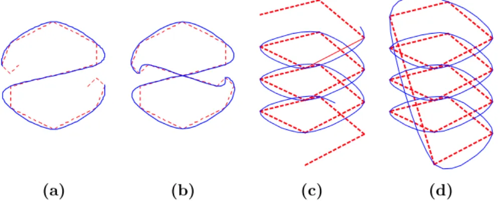
(a) (b) (c) (d)
Figure 3. Open case (a) and close case (b) of Example 2; open case (c) and close case (d) of Example 3.
Two examples as shown in Figures 3 are used to illustrate the efficiency of the data decompression algorithms. The digital curves in Examples 2 and 3 are of two dimensions and three dimensions, respectively. In the open case of Example 3, the digital curve as shown in Figure 3 (c) is a three-dimensional
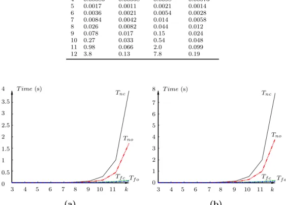
Table 2. Performance of approaches on Example 3. k Tno(s) Tf o(s) Tnc(s) Tf c(s) 3 0.00038 0.00031 0.00042 0.00037 4 0.00086 0.00058 0.0098 0.00073 5 0.0017 0.0011 0.0021 0.0014 6 0.0036 0.0021 0.0054 0.0028 7 0.0084 0.0042 0.014 0.0058 8 0.026 0.0082 0.044 0.012 9 0.078 0.017 0.15 0.024 10 0.27 0.033 0.54 0.048 11 0.98 0.066 2.0 0.099 12 3.8 0.13 7.8 0.19 0 0.5 1 1.5 2 2.5 3 3.5 4 T ime (s) 3 4 5 6 7 8 9 10 11 k Tnc Tno Tf c Tf o 0 1 2 3 4 5 6 7 8 T ime (s) 3 4 5 6 7 8 9 10 11 k Tnc Tno Tf c Tf o (a) (b)
Figure 4. Performance of approaches on: (a) Example 2, and (b) Example 3.
spiral. The polygonal curves or the polygons formed by M0 are dashed in those two figures, and the solid curves are the results after several iterate subdivision steps. The numbers of the control points in M0 of Examples 2 and 3 are 14 and 21, respectively. Tables 1 and 2 give the time cost of the approaches on Examples 2 and 3, which are illustrated in Figure 4 as well. In the tables and the figure, k represents for the iterate subdivision steps.
Tno and Tnc represent for the time cost with the method given by [4] on the
open curves and the closed curves, respectively. Tf oand Tf c represent for the
time cost by Algorithm 3 on the open curves and Algorithm 4 on the closed curves, respectively. All the data are calculated on a personal computer with 2.8 GHz CPU and 1G memory. The programming language is C++. As shown in Tables 1 and 2, the new approaches are much faster than the traditional method in [4].
6 Conclusions
This paper provides adaptive geometry compression methods with labels based on 4-point interpolatory subdivision schemes. It can work on digital curves of arbitrary dimensions, for example, d dimensions if the points are all of
d−dimensions. The examples shown in Figures 2 and 3(d) show that the data
compression ratios could be about 32 : 1. For decompressing the compressed data, this paper as well provides high-speed 4-point interpolatory subdivision curve generation methods such that decompression could be performed effi-ciently. As shown in the examples, the new approaches are able to reduce the time cost sharply. The high-speed 4-point interpolatory subdivision curve generation methods not only take advantages to data decompression, but also give great benefit to the real-time display and interaction of 4-point subdivi-sion curves.
Acknowledgements
The research was supported by Chinese 973 Program(2004CB719400), and the National Science Foundation of China (60403047, 60533070). The second author was supported by the project sponsored by a Foundation for the Au-thor of National Excellent Doctoral Dissertation of PR China (200342), and a Program for New Century Excellent Talents in University(NCET-04-0088). References
[1] H Biermann, D Kristjansson, and D Zorin. Approximate Boolean operations on free-form solids. In Proceedings of SIGGRAPH, pages 185–194, 2001.
[2] G Chaikin. An algorithm for high-speed curve generation. Computer Graphics and Image
Pro-cessing, 3:346–349, 1974.
[3] F Cheng and J-H Yong. Subdivision depth computation for Catmull-Clark subdivsion surfaces.
Computer-Aided Design and Applications, 3(1-4):485–494, 2006.
[4] N Dyn, D Levin, and JA Gregory. A 4-point interpolatory subdivision scheme for curve design.
Computer Aided Geometric Design, 4(4):257–268, 1987.
[5] MF Hassan, IP Ivrissimitzis, NA Dodgson, and MA Sabin. An interpolating 4-point C2ternary
stationary subdivision scheme. Computer Aided Geometric Design, 19(1):1–18, 2002.
[6] A Khodakovsky, P Schroder, and W Sweldens. Progressive geometry compression. In Proceedings
of SIGGRAPH, pages 271–278, 2000.
[7] Z Ma, N Wang, G Wang, and S Dong. Multi-stream progressive geometry compression. Journal
of Computer-Aided Design & Computer Graphics, 18(2):200–207, 2006.
[8] J Stam. Exact evaluation of Catmull-Clark subdivision surfaces at arbitrary parameter values. In Proceedings of SIGGRAPH, pages 395–404, 1998.
[9] J-H Yong and F Cheng. Adaptive subdivision of Catmull-Clark subdivision surfaces.
Computer-Aided Design and Applications, 2(1-4):253–261, 2005.
[10] J-H Yong, S-M Hu, and J-G Sun. Degree reduction of uniform B-spline curves. Chinese Journal
of Computers, 23(5):537–540, 2000.
[11] J-H Yong, S-M Hu, and J-G Sun. CIM algorithm for approximating three-dimensional polygonal curves. Journal of Computer Science and Technology, 16(6):552–559, 2001.
[12] J-H Yong, S-M Hu, J-G Sun, and X-Y Tan. Degree reduction of B-spline curves. Computer Aided
[13] H Zhang, J-H Yong, and J-C Paul. Adaptive geometry compression based on 4-point interpola-tory subdivision schemes. Lecture Notes in Computer Science, 4153:425–434, 2006.
[14] J Zhang and CB Owen. Octree-based animated geometry compression. In Data Compression
Conference, pages 508–517, 2004.
[15] D Zorin and P Schr¨oder. Interactive multi-resolution mesh editing. In Proceedings of