Analysis and Modeling of Non-Native Speech
for Automatic Speech Recognition
by
Karen Livescu
A.B., Princeton University (1996)
Submitted to the Department of Electrical Engineering and Computer Science
in partial fulfillment of the requirements for the degree of
Master of Science
at the
MASSACHUSETTS INSTITUTE OF TECHNOLOGY
August 1999
@
Massachusetts Instituteo Technology 1999. All rights reserved.
A u th o r ...
Department of Electrical Engineering and Computer Science
August 13, 1999
Certified by...
.... ... ..
nes R. Glass
Principal Research Scientist
Thesis Supervisor
A ccepted by ... .. ...
Arthur C. Smith
Chairman, Departmental Committee on Graduate Students
MASSACHUSETTS
INSTITUTE
OF TECHNOLOGYAnalysis and Modeling of Non-Native Speech
for Automatic Speech Recognition
by Karen Livescu
Submitted to the Department of Electrical Engineering and Computer Science on August 13, 1999, in partial fulfillment of the requirements for the degree of
Master of Science
Abstract
The performance of automatic speech recognizers has been observed to be dramatically worse for speakers with non-native accents than for native speakers. This poses a problem for many speech recognition systems, which need to handle both native and non-native speech. The problem is further complicated by the large number of non-native accents, which makes modeling separate accents difficult, as well as the small amount of non-native speech that is often available for training. Previous work has attempted to address this issue by building accent-specific acoustic and pronunciation models or by adapting acoustic models to a particular non-native speaker.
In this thesis, we examine the problem of non-native speech in a speaker-independent, large-vocabulary, spontaneous speech recognition system for American English, in which a large amount of native training data and a relatively small amount of non-native data are available. We investigate some of the major differences between native and non-native speech and attempt to modify the recognizer to better model the characteristics of
non-native data. This work is performed using the SUMMIT speech recognition system in the
JUPITER weather information domain.
We first examine the modification of acoustic models for recognition of non-native speech. We show that interpolating native and non-native models reduces the word error rate on a non-native test set by 8.1% relative to a baseline recognizer using models trained on pooled native and non-native data (a reduction from 20.9% to 19.2%). In the area of lexical modeling, we describe a small study of native and non-native pronunciation using manual transcriptions and outline some of the main differences between them. We then attempt to model non-native word pronunciation patterns by applying phonetic substitutions, dele-tions, and insertions to the pronunciations in the lexicon. The probabilities of these phonetic confusions are estimated from non-native training data by aligning automatically-generated phonetic transcriptions with the baseline lexicon. Using this approach, we obtain a relative reduction of 10.0% in word error rate over the baseline recognizer on the non-native test
set. Using both phonetic confusions and interpolated acoustic models, we further reduce the word error rate to 12.4% below baseline. Finally, we describe a study of language model differences between native and non-native speakers in the JUPITER domain. We find that, within the resolution of our analysis, language model differences do not account for a sig-nificant part of the degradation in recognition performance between native and non-native test speakers.
Thesis Supervisor: James R. Glass Title: Principal Research Scientist
Contents
1 Introduction 11
1.1 Previous W ork . . . . 12
1.2 Goals and Overview . . . . 13
2 The JUPITER Domain and SUMMIT Recognizer 15 2.1 JUPITER ... . ... 15
2.1.1 The JUPITER Corpus . . . . 15
2.1.2 Division of the Corpus into Training, Development, and Test Sets . 17 2.2 SUMMIT ... ... - . . - -18
2.2.1 Segm entation . . . .. 19
2.2.2 Acoustic M odeling . . . . 20
2.2.3 Lexical M odeling . . . . 20
2.2.4 Language Modeling . . . . 21
2.2.5 Searching for the Best Hypothesis . . . . 21
2.2.6 Recognition Using Finite-State Transducers . . . . 22
2.3 The Baseline Recognizer . . . . 22
2.3.1 Acoustic M odels . . . . 22
2.3.2 The Lexicon . . . . 23
2.3.3 The Language Model . . . . 23
2.3.4 Baseline Performance . . . . 23
3 Acoustic Modeling 25 3.1 Native and Non-Native Acoustic Models . . . . 25
3.2 M odel Interpolation . . . . 26
3.2.1 D efinition . . . .. . . . . . . 27
3.2.2 Experim ents . . . . 27
4 Comparison of Native and Non-Native Lexical Patterns Using Manual Transcriptions 31 4.1 Manual Transcriptions . . . . 31
4.1.1 Guidelines for Preparation of Transcriptions . . . . 32
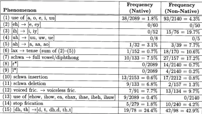
4.2 Observations on Common Pronunciation Phenomena in Transcriptions . . . 33
4.2.1 Non-Native Speakers . . . . 33
4.2.2 Native Speakers . . . . 34
5 Automatic Acquisition of Non-Native Pronunciation Patterns
5.1 A pproach . . . . . 40
5.2 M ethods . . . . 42
5.2.1 Estimation of CFST Arc Probabilities . . . . 42
5.2.2 Computational Considerations of CFST's . . . . 44
5.2.3 The Sparse Data Problem . . . . 44
5.3 Experim ents . . . . 46
5.3.1 Training from Phonetic Recognition Hypotheses . . . . 46
5.3.2 Training from Forced Paths . . . . 52
5.3.3 Iterative Training . . . . 55
5.3.4 Comparison of Smoothing Approaches . . . . 57
5.3.5 Recognition with Interpolated Models and CFST's . . . . 59
5.4 Sum m ary . . . . 60
6 Effect of the Language Model on Recognition Performance 63 6.1 Experimental Setup . . . . 64
6.2 Set Log Probabilities . . . . 64
6.3 Per-Speaker PNLP's . . . . 65 6.4 Sum m ary . . . . 69 7 Conclusion 71 7.1 Sum m ary . . . . 71 7.2 Future W ork . . . . 73 A Label Sets 79 B Confusion Matrices 83 39
List of Figures
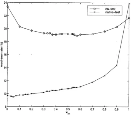
3-1 Word error rates obtained on native and non-native development sets using
interpolated models with varying relative weights. . . . . 28
3-2 Word error rates obtained on native and non-native test sets using interpo-lated models with varying relative weights. . . . . 30
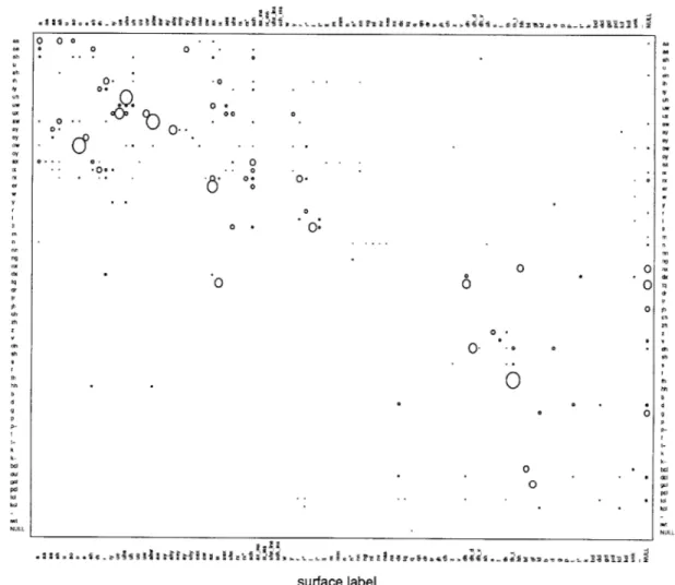
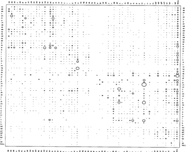
4-1 Bubble plot showing the estimated confusion probabilities for non-native speakers. The radius of each bubble is proportional to the probability of the corresponding confusion. The largest bubble corresponds to P(th-tlth) = 0.4545. . . . . 36
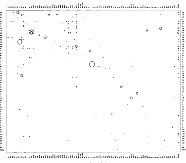
4-2 Bubble plot showing the estimated confusion probabilities for native speakers. The largest bubble corresponds to P(llll) = 0.5833. The scale is the same in this plot as in Figure 4-1. . . . . 37
5-1 Example portion of a simple C. . . . . 40
5-2 Lexical pronunciation graph for the word Chicago. . . . . 41
5-3 Expanded lexical pronunciation graph for the word Chicago. . . . 41
5-4 Bubble plot showing the estimated confusion probabilities using the phonetic recognition method. The radius of each bubble is proportional to the prob-ability of the corresponding confusion. The largest bubble corresponds to P (ch : t) = 0.155. . . . . 48
5-5 Average number of arcs per phone as a function of CFST pruning threshold, using the phonetic recognition method . . . . . 50
5-6 Word error rate on nn-dev as a function of CFST pruning threshold, using the phonetic recognition method. . . . . 50
5-7 Word error rate on nn-test as a function of CFST pruning threshold, using the phonetic recognition method. . . . . 51
5-8 Bubble plot showing the confusion probabilities derived from alignments of forced paths obtained on the non-native training set. The largest bubble corresponds to P(tq : NULL) = 0.2174. . . . . 53
5-9 Average number of arcs per phone as a function of CFST pruning threshold, using the forced paths method. . . . . 56
5-10 Word error rate on nn-dev as a function of CFST pruning threshold, using the forced paths method. . . . . 56
5-11 Word error rate on nn-test as a function of CFST pruning threshold, using the forced paths method. . . . . 57
5-12 Average number of arcs per phone as a function of CFST pruning threshold, using the forced paths method, for 1", 2"d, and 3rd iterations . . . . 58
5-13 Word error rate on nn-dev as a function of CFST pruning threshold, using the forced paths method, for 1"t, 2nd, and 3rd iteration. . . . . 58
5-14 Word error rate on nn-dev as a function of CFST pruning threshold, us-ing either the baseline acoustic models or interpolated acoustic models with
w nn = 0.54. . . . . 60 5-15 Word error rate on nn-test as a function of CFST pruning threshold,
us-ing either the baseline acoustic models or interpolated acoustic models with
w on = 0.54. . . . . 61 6-1 Scatterplot of WER versus PNLP for the native test set. . . . . 66 6-2 Scatterplot of WER versus PNLP for the non-native test set. . . . . 66 6-3 Histograms of WER and PNLP for the native and non-native test sets. . . . 67 6-4 Average WER versus PNLP for native and non-native speakers, along with
List of Tables
2-1 Example of a conversation with JUPITER. . . . .. 16 2-2 Breakdown of the JUPITER corpus into accent classes and in-vocabulary
ver-sus out-of-vocabulary utterances. . . . . 17 2-3 Number of utterances in the training, development, and test sets. The
ab-breviations used in this table are: nn = non-native; dev = development; iv = in-vocabulary. The pooled-train-iv set is the subset of pooled-train consisting of only the in-vocabulary utterances. . . . . 18 2-4 Rates of substitution (S), insertion (I), and deletion (D) and word error rates
(WER) obtained with the baseline recognizer on native and non-native sets. Each error rate is a percentage of the number of reference (actual) words in the test set. . . . . 24 3-1 Rates of substitution (S), insertion (I), and deletion (D) and word error rates
(WER) for recognizers using the native, non-native, and pooled acoustic models. The sets are the native and non-native development sets (native-dev, and nn-(native-dev, respectively). . . . . 26 3-2 Comparison of error rates on the non-native test set obtained with the
base-line models, non-native models, and interpolated models with w," = 0.54 . 29 3-3 Comparison of error rates on the native test set obtained with the baseline
models, native models, and interpolated models with wn = 0.03 . . . . 29 4-1 Frequencies of various phenomena noted in manual transcriptions of native
and non-native data. . . . . 38 5-1 Rates of substitution (S), insertion (I), and deletion (D) and word error rates
(WER) on nn-dev for recognizers using the baseline lexicon and a lexicon with arc weights trained on nn-train. In both cases, the baseline acoustic m odels were used. . . . . 39 5-2 Frequency and most common confusions for each lexical label, using the
phonetic recognition method. . . . .. 49 5-3 Error rates obtained on nn-test using a CFST with cprune = 4, trained
using the phonetic recognition method. . . . . 51 5-4 Frequency and most common confusions for each lexical label, using the
forced paths method. . . . . 54 5-5 Error rates obtained on nn-test using a CFST, forced paths method. In this
test, cprune = 12, vprune = 15, wtw = 2. . . . . 55 5-6 Comparison of error rates on nn-dev using various types of smoothing. In
5-7 Error rates obtained on nn-test using a CFST, forced paths method, with interpolated acoustic models. In this test, cprune = 12, vprune = 15, wtw
= 2. ... ... 59
5-8 Summary of the main results on nn-dev and nn-test. The methods com-pared are: Baseline recognizer; PR = baseline recognizer with CFST trained using phonetic recognition method; FP = baseline recognizer with CFST trained using forced paths method; Interpolated AM = baseline recognizer using interpolated acoustic models with won = 0.54; and FP+Interp. AM =
CFST trained using forced paths method + interpolated acoustic models. 61 6-1 PNLP's, perplexities, and WER's for the native and non-native test sets. . 65
7-1 Error rates obtained on nn-test using the baseline recognizer, interpolated acoustic models (AM), a CFST trained using the forced paths (FP) method, and both interpolated AM and a CFST. The CFST in this table is CFP,
unpruned and padded with the pad-1 method. . . . . 72 A-1 Label set used for baseline recognizer in Chapters 2-5. . . . . 80 A-2 Labels used for manual transcriptions which are not included in Table A-1.
The label descriptions are often given in terms of other labels in this table or in Table A-1. For diphthongs, the descriptions are of the form [starting point]-[ending point]. The transcriptions made use of all of the labels shown here and all of the labels in Table A-1, with the following exceptions: [er] was not used-[rx] was used to represent both [er] and [rx]; and no distinction was made between aspirated and unaspirated stops, using the labels for the aspirated stops to represent both levels of aspiration. The labels were created as needed, so that some are only used in the native transcriptions, while others are only used in the non-native transcriptions. . . . . 81 B-1 Confusion matrix showing the frequency of each confusion and the total frequency
of each lexical label, using the phonetic recognition method. Lexical labels are on
the left and right; surface labels are listed along the top and bottom. The table is
continued on the following page. . . . . 84 B-1 Confusion matrix obtained with the phonetic recognition method (continued). . . 85 B-2 Confusion matrix showing the frequency of each confusion and the total frequency
of each lexical label, using the forced paths method. Lexical labels are on the left and right; surface labels are listed along the top and bottom. This table is continued on the following page. . . . . 86 B-2 Confusion matrix obtained with the forced paths method (continued). . . . . 87
Chapter 1
Introduction
The study of automatic recognition of non-native speech is motivated by several factors. First, any deployed speech recognizer must be able to handle all of the input speech with which it is presented, and in many cases, this includes non-native as well as native speech. Recognition accuracy has been observed to be drastically lower for non-native speakers of the target language than for native ones [12, 29, 31]. Research on both non-native accent modeling and dialect-specific modeling, a closely related issue, shows that large gains in performance can be achieved when the acoustics [3, 8, 22, 31] and pronunciation [15, 21, 29] of a new accent or dialect are taken into account. A motivation for studying non-native speech in particular, as opposed to dialect, is that non-native speech has been less widely studied and has some specific properties [16] that appear to be fundamentally different from those of dialectal speech. From a speech recognition perspective, non-native accents are more problematic than dialects because there is a larger number of non-native accents for any given language and because the variation among speakers of the same non-native accent is potentially much greater than among speakers of the same dialect.
The problem of recognition of non-native speech is one of mismatch between the recog-nizer's expectations and the test data. This includes two kinds of mismatch. The first is mismatch between models automatically determined from training data and the character-istics of the test data. The second is mismatch between knowledge-based, hand-made or partially hand-made models (for example, for word pronunciation) and the corresponding aspects of the test data. It has been previously observed that the performance of a speech recognizer varies with the degree of similarity between the data on which its models have been trained and the data on which it is tested. For example, in the case of the JUPITER conversational system (described in Chapter 2), the training data for the deployed system consists largely of native or lightly accented adult male speakers of American English; as a result, performance is significantly worse for female speakers, children, and non-native speakers with heavy accents [12]. A similar effect has been noted for recognizers trained on one dialect and tested on another dialect of the same language [8, 15].
1.1
Previous Work
Perhaps the simplest way to address the problem of training/testing mismatch is to pool the native training data with any available non-native training data. This approach treats native and non-native data as equivalent. As we show in Chapter 3, this can improve recognition of non-native speech relative to acoustic models trained on native data and even upon that of models trained on only native data, presumably because the non-native training data alone are insufficient to train robust models. This does not eliminate the mismatch, but it ensures that the recognizer has seen at least some training data similar to the test data.
Another approach to the problem of mismatch is to use multiple models, with each model optimized for a particular accent or class of accents. An accent-independent recognizer can then be built by using an accent classifier to detect the accent of a test speaker and then recognizing with the appropriate models. This approach is most commonly applied to the acoustic model. If there are sufficient training data for each accent class, separate acous-tic models can be trained on accent-specific data. This method has been applied with some success to the recognition of both non-native accents [29] and dialectal accents [3]. In [29], Teixeira et al. show an improvement in isolated-word recognition over baseline British-trained models, using both whole-word and subword models and using either sev-eral accent-specific models or a single model for all non-native accents. Beattie et al. [3] compare gender- and dialect-dependent models to a baseline model trained on pooled multi-dialect data in a small-vocabulary (about 200-word) continuous speech recognition task for American English. In this work, the gender-dependent and gender- and dialect-dependent models achieved higher recognition accuracy than the pooled.
Very often, however, it is difficult to obtain sufficient data to robustly train the accent-specific models. In these cases, model adaptation is often used. In this approach, a single set of initial models is trained on a large set of data, but some transformation of the models is performed based on a smaller set of adaptation data from a single speaker or speaker category, determined by characteristics such as gender or accent. The adaptation can be either supervised, in which a set of previously transcribed data is used, or unsupervised, in which the recognizer's output is used to transform the models. This approach has been used, for example, by Diakoloukas et al. [8] to build a set of dialect-specific models for a new dialect of Swedish by adapting a set of existing models for another dialect with various amounts of development data. In this work, the adapted models are shown to outperform both the original unadapted models and a set of models trained only on data from the new dialect. Adaptation has also been used successfully to build speaker-dependent models for non-native speakers, using both supervised [3, 22, 31] and unsupervised [22, 31] approaches. In the area of lexical modeling, several attempts have been made to better account for non-native word pronunciations. Liu and Fung [21], for example, obtain an improvement in recognition accuracy on English speakers with a Hong Kong accent by expanding a native lexicon using phonological rules based on knowledge of the speakers' native Cantonese. Teixeira et al. [29] use a data-driven approach to customize word pronunciation to specific non-native accents, using the Baum-Welch algorithm to retrain expanded hidden-Markov models representing the allowable pronunciations. Similar approaches have also been used
for dialect-specific recognition. Humphries et al. [15], for example, use a tree clustering method to train probabilistic phonological rules for one British dialect and apply these rules to an existing lexicon designed for another dialect.
1.2
Goals and Overview
In the previous work we have mentioned, most of the approaches have involved modeling either a particular accent or a particular speaker. In this thesis, we investigate speaker-independent recognition, with no speaker adaptation. For a system dealing with non-native speakers from many diverse backgrounds, however, an approach using accent-specific models has two major disadvantages. First, in order to effectively account for all of the different accents of the test speakers, the number of models must be very large. This means both that the models are more computationally cumbersome and that a much larger set of training data is needed to adequately cover all of the accent categories. This problem is more marked for non-native accents than for dialectal accents because, typically, there are many fewer dialects of a given language than there are non-native accents. Furthermore, whereas dialects appear to be fairly stable and predictable, there can be marked differences between non-native speakers with the same accent. These differences are due to different levels of familiarity with the target language, as well as individual tendencies in mapping unfamiliar sounds and linguistic rules.
For these reasons, we are interested in the insights and performance gains we can obtain by analyzing and modeling all non-native speakers as a single group. Specifically, the main goals of this thesis are:
" To understand, in a qualitative and quantitative way, some of the major differences between native and non-native speakers of American English and the ways in which they affect the performance of a speech recognizer
" To investigate modifications to a speech recognizer geared toward improving its per-formance on non-native speakers
From the point of view of improving recognition performance, the main question we would like to address is: When faced with a domain in which we have a large amount of native data and a small amount of varied non-native data, how can we best use the limited non-native data to improve the recognizer's performance as much as possible? Although we occasionally examine the effects of our methods on the recognition of native speech, we do not attempt to build an accent-independent speech recognition system, that is, one that can handle both native and non-native speakers. Our main concern is to improve the recognition of non-native speech.
Chapter 2 describes the domain in which the work was performed and the baseline speech recognizer. The remainder of the thesis is divided into three parts, corresponding roughly to the three main components of a speech recognition system: Acoustic modeling, lexical modeling, and language modeling. Chapter 3 discusses experiments performed on the
acoustic models. Chapters 4 and 5 discuss issues in lexical modeling: Chapter 4 describes a study of pronunciation patterns using manual transcriptions of native and non-native data, and Chapter 5 describes a method for automatic acquisition of such patterns and incorporation of this knowledge into the recognizer. Chapter 6 describes measurements showing the effect of language model differences between native and non-native speakers on the performance of the recognizer. Chapter 7 summarizes the thesis and suggests directions for future work.
Chapter 2
The
JUPITER
Domain
and SUMMIT
Recognizer
All of the work described in this thesis was performed in the JUPITER weather domain using the SUMMIT speech recognition system. The following sections describe the JUPITER conversational system and the associated database; the SUMMIT recognizer; and the baseline recognizer used for most of the experiments in the following chapters.
2.1 JUPITER
JUPITER is a telephone-based conversational system providing weather-related information for approximately 500 cities worldwide [33, 12, 11]. Using a toll-free number, users call JUPITER and inquire about various aspects of current weather forecasts, such as tempera-ture, humidity, wind speed, precipitation, sunrise and sunset times, and weather advisories. In addition, users can ask JUPITER for help or clarification in various ways, such as "What cities do you know in New Jersey?", "What can I ask?", or "Repeat that please." During a call, JUPITER keeps a history of dialogue-specific information, so that questions such as "What about tomorrow?" can be answered appropriately, depending on the city and type of information that have been established in previous queries. Table 2-1 shows an example of a successful JUPITER conversation.
2.1.1
The
JUPITERCorpus
Calls made to JUPITER are stored in a database, or corpus, for training and system develop-ment. The corpus used in this thesis contains 62,324 utterances collected between February 1997 and July 1998. Most of the utterances were collected live via the toll-free number. The corpus also contains approximately 3,500 read utterances, as well as about 1,000 ut-terances obtained through wizard data collection, in which the input is spontaneous but a
User: I'd like the weather in New York.
JUPITER: I know of the following places in New York: Albany, Binghamton, Buffalo, Elmira, Ithaca, New York City, Niagara Falls, Rochester, Syracuse, Utica, and Water-town. Please select one.
User: Albany.
JUPITER: In Albany today: Patchy fog early. Very warm and hazy and humid. Scattered showers early this morning. A little sunshine midday with chance of more showers and thunderstorms in the later afternoon. High upper 80s. 30 percent chance of rain. Tonight: Showers likely and possibly thunderstorms. Lows upper 60s. 60 percent chance of rain. Is there something else I can do for you?
User: Tomorrow's weather.
JUPITER: In Albany Friday: 30 percent chance of shower morning. Then clouds mixing with increasing sunshine afternoon. Becoming less humid. High lower 80s. What else would you like to know?
User: Nothing thank you.
JUPITER: Thanks for using JUPITER! Have a nice day!
Table 2-1: Example of a conversation with JUPITER.
human typist replaces the computer [12]. In our experiments, we used only the live data for training and testing. For each utterance, the corpus contains an orthographic transcription produced by a human transcriber.
In order to study native and non-native speech separately, we tagged each utterance in the corpus with an accent class label. We used the following accent classes: amer for native-sounding speakers of American English; uk-aus for native-native-sounding speakers of another dialect of English such as British or Australian English; other for all non-native speakers of English; and undef to indicate that the accent is "undefined", which we define below. We classified the accents by listening to those utterances which were noted by the transcriber as being possibly non-native, British, or Australian. We tagged an utterance as other whenever we could discern a non-native accent, whether weak or strong.
We note the following details about the classification of accents. First, we treat the uk-aus accent class as neither native nor non-native. This is because, while these speakers are not native speakers of American English, they are native speakers of another dialect of English and are not attempting to approximate American English. Although the acoustics, pronunciation, syntax, and semantics of non-American English dialects are all to some extent different from those of American English, they are presumably both more predictable and more similar to those of American English than are those of non-native English. For these reasons, the uk-aus utterances were excluded from further analysis. We use the term "non-native" to describe only those speakers whose accent is labeled other in the corpus, and the term "native" to describe only the amer utterances.
Second, we assume that all non-native speakers in the corpus are attempting to speak
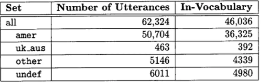
Set Number of Utterances In-Vocabulary all 62,324 46,036 amer 50,704 36,325 uk-aus 463 392 other 5146 4339 undef 6011 4980
Table 2-2: Breakdown of the JUPITER corpus into accent classes and in-vocabulary versus out-of-vocabulary utterances.
such as British or Australian English, we assume that the differences between non-native approximations of different English dialects are no larger than, or qualitatively different from, the differences between various non-native approximations of American English. We therefore treat all non-native speakers as a single group in our analysis and experiments.
The undef accent was applied to all:
1. Read (non-spontaneous) utterances. We perform all analysis and experiments only on spontaneous speech; because of the time-consuming nature of manual accent clas-sification, we classified only spontaneous utterances.
2. Utterances spoken in a language other than English.
3. Utterances for which the accent class could not be determined for any reason; for example, because the utterance was too short or noisy to discern the accent, the speaker seemed to be using an artificial accent, or the recording contained only non-speech sounds.
Table 2-2 shows the number of utterances in the corpus in each of the accent classes. The table also contains the number of in-vocabulary utterances in each accent class, which are those utterances that contain only words within the 1956-word JUPITER vocabulary.
2.1.2 Division of the Corpus into Training, Development, and Test Sets
We divided the native and non-native utterances in the corpus into training, development, and test sets. The training sets were used to train acoustic and language models, as well as lexicon arc weights and the phonetic confusion weights discussed in Chapter 5. The development sets are used to perform intermediate tests, during which various parameters may be optimized. The test sets are used to obtain the final results and are not tested on or analyzed prior to the final experiments. The utterances in a single call to JUPITER are always placed in the same set, so that we do not test on utterances from calls on which we have trained. However, since the same speaker may call more than once, and since we do not know the identity of the speaker(s) in each call, the development and test sets may contain some of the same speakers as the training sets.
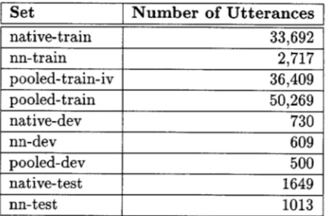
Set Number of Utterances native-train 33,692 nn-train 2,717 pooled-train-iv 36,409 pooled-train 50,269 native-dev 730 nn-dev 609 pooled-dev 500 native-test 1649 nn-test 1013
Table 2-3: Number of utterances in the training, development, and test sets. The abbrevia-tions used in this table are: nn = non-native; dev = development; iv = in-vocabulary. The pooled-train-iv set is the subset of pooled-train consisting of only the in-vocabulary utterances.
Table 2-3 shows the number of utterances in each of these sets. All of the sets except pooled-train contain in-vocabulary utterances only. The pooled-train-iv set is simply the union of native-train and nn-train. The pooled-dev set is a random 500-utterance subset of the union of native-dev and nn-dev.
2.2 SUMMIT
SUMMIT is a segment-based speech recognition system [9]. That is, it attempts to segment the waveform into predefined subword units, which may be phones, sequences of phones, or parts of phones. This is in contrast to frame-based recognizers, which divide the waveform into equal-length windows, or frames [2, 24]. Both approaches first extract acoustic features at small, regular intervals. However, segment-based recognition approaches next attempt to segment the waveform using these features, while based recognizers use the frame-based features directly.
The problem that a continuous speech recognizer attempts to solve is: For a given input waveform with corresponding acoustic feature vectors A = {d1, d2,... , dN}, what is the
most likely string of words '* = {wi, w2,. , WM} that produced the waveform? In other
words,
w* =argmaxP(9|A), (2.1)
where w' ranges over all possible word strings. Since a single word string may be realizable as different strings of units Ui with different segmentations s, this equation becomes:
G* = arg max WP(, , s,A), (2.2)
t9
8
U'ssegmen-tations for all of the pronunciations. This summation can be computationally expensive. As a simplification, SUMMIT assumes that, given a word sequence ', there is an optimal segmentation and unit sequence, which is much more likely than any other s and it. The summation is therefore replaced by a maximization, in which we attempt to find the best triple of word string, unit sequence, and segmentation, or the best path, given the acoustic features:
{Gj* *, s*} = arg
max
P( ,, s,
A) (2.3)Applying Bayes' Rule several times, this can be rewritten as
= arrnxP(A, it,
s)P(sl,
z)P(ilz|)P(
')
{ 7 , *, s }= arg max , (2.4)
,s P(A)
= arg max P(Al, it, s)P(sli, z)P(i|lwi)P(zI) (2.5)
The second equality arises from the fact that P(A) is constant for all W', it, and s, and therefore does not affect the maximization.
This derivation describes the approach used in Viterbi decoding [2], and is identical for frame-based and based recognizers. The difference lies in the fact that segment-based recognizers explicitly consider segment start and end times during the search, whereas frame-based methods do not. Segment-based methods can therefore require significantly more computation during the search.
The estimation of the four components of the last equation is performed by, respectively, the acoustic, duration, lexical (or pronunciation), and language model components. In this thesis, we do not use a duration model; that is, P(s|li, W') is constant. The following four sections describe the other components of the SUMMIT recognizer: segmentation, acoustic modeling, lexical modeling, and language modeling. We finally describe the methods SUM-MIT uses to search for the best path and the implementation of SUMSUM-MIT using finite-state transducers.
2.2.1 Segmentation
One way to limit the size of the search space is to transform the input waveform into a constrained network of hypothesized segments. In SUMMIT, this is done by first extracting frame-based acoustic features (e.g., MFCC's) at small, regular intervals, as in a frame-based recognizer, and then hypothesizing groupings of frames which define possible segments. There are various methods for performing this task; two that have been used in SUMMIT are acoustic segmentation [10, 19], in which segment boundaries are hypothesized at points of large acoustic change, and probabilistic segmentation [5, 19], which uses a frame-based phonetic recognizer to hypothesize boundaries. In this thesis, we use acoustic segmentation.
2.2.2
Acoustic Modeling
After segmentation, a vector of acoustic features is extracted for each segment or boundary in the segmentation graph, or for both the segments and boundaries in the graph. In this thesis, we use only the boundaries in the segment graph. Each hypothesized boundary in the graph may be an actual transition boundary between subword units, or an internal "boundary" within a phonetic unit. We refer to both of these as boundaries or diphones, although the latter kind does not correspond to an actual boundary between a pair of phones.
The acoustic features are now represented as a set of boundary feature vectors Z =
{1, 22, ... , iLI. SUMMIT assumes that boundaries are independent of each other and of the
word string, so that the acoustic component in (2.5) becomes
L
P(ZIz5<7,s) = HP(ZI|,s) (2.6)
l=1
We further assume that the conditional probability of each it is independent of any part of u and s other than those pertaining to the lth boundary, so that
L
P (Z|G I -,U s) = PjzI|bi), ( (2.7)
l=1
where bi is the l'h boundary label as defined by U' and s. The vector function of probabilities of feature vectors Z conditioned on boundary labels bi from a set of R boundary labels,
P(zbi) P(zb2)
PP) . (2.8)
.P(z bR)
is estimated by the acoustic model, or set of acoustic models if we wish to emphasize the fact that each bi is modeled separately. During recognition, the acoustic model assigns to each boundary in the segmentation graph a vector of scores corresponding to the probability of observing the boundary's features given each of the bi. In practice, however, not all of the scores may be generated for each boundary. Instead, the scores are computed on demand, generating scores only for the hypotheses that are being considered in the recognition search at a given time.
2.2.3 Lexical Modeling
Lexical modeling is represented by the lexicon, a dictionary of allowable pronunciations for all of the words in the recognizer's vocabulary [32]. The lexicon consists of one or more basic pronunciations, or baseforms, for each word, as well as any number of alternate pronunciations created by applying phonological rules to the baseform. The phonological rules account for processes such as place assimilation, gemination, and alveolar stop flapping.
The alternate pronunciations are represented as a graph. In addition, the arcs in the lexicon can be weighted to account for the different probabilities of the alternate pronunciations. The lexical probability component in (2.5) is therefore the probability of a given path in the lexicon.
2.2.4
Language Modeling
The language model provides an estimate of P('), the probability of observing the word sequence w. One widely-used class of language models is n-grams [2]. The probability of an N-word string can be rewritten as
N
P() =
HP(wilwi1,
wi-2,- ,wi) (2.9)i=1
n-grams assume that the probability of a given word depends on a finite number n - 1 of preceding words:
N
P(?5) =
IP(wilwi_1,
wi-2, ...
, Win-1)) (2.10)The probability estimates for n-gram language models are typically trained by counting the number of times each n-word sequence occurs in a set of training data. To deal with the problem of n-grams that do not occur in the training data, smoothing methods are often used to redistribute some of the probability from observed n-grams to unobserved
n-grams [6]. In all of the experiments in this thesis, we use word n-grams with n = 2 or n = 3, referred to as bigrams and trigrams, respectively.
2.2.5 Searching for the Best Hypothesis
During recognition, the combined constraints of the scored segmentation graph, the lexicon, and the language model produce a weighted graph representing the search space. The recognizer must then find the best-scoring path through this graph. In the version of SUMMIT used in this thesis, the language model is applied in two passes. In the first pass, a forward Viterbi beam search [25] is used to obtain the partial-path scores to each node using a bigram language model, followed by a backward A* beam search [30] using the scores from the Viterbi search as the look-ahead function. The A* search produces a smaller word graph, which can then be searched with a more computationally demanding language model such as a trigram. In the second pass, the new language model is used to rescore the word graph with forward partial path scores, and a backward A* search is again used to obtain the final hypotheses.
2.2.6
Recognition Using Finite-State Transducers
For most of our recognition experiments, we used an implementation of SUMMIT using weighted finite-state transducers, or FST's [11]. An FST recognizer R can be represented as the composition of four FST's,
R = A oD o L o G, (2.11)
where: A is a segment graph with associated acoustic model scores; D performs the con-version from the diphone labels in the acoustic graph to the phone labels in the lexicon; L represents the lexicon; and G represents the language model. The process of recognition then becomes a search for the best path through R. SUMMIT allows the composition of D, L, and G to be performed either during or prior to recognition.
2.3
The Baseline Recognizer
This section describes the baseline recognizer used in all of the experiments other than the ones pertaining to the language model; see Chapter 6 for a description of the baseline recognizer used in the language model experiments.
2.3.1 Acoustic Models
The features used in the acoustic models are the first 14 Mel-frequency cepstral coefficients (MFCC's) averaged over 8 different regions near each boundary in the phonetic segmen-tation of each utterance [11]. These 112 features (14 MFCC's x 8 regions) are reduced to a 50-dimensional vector using principal components analysis (PCA). The PCA trans-forms the resulting feature space, producing an identity covariance matrix for the training data [4]. The acoustic models are diagonal Gaussian mixture models with up to 50 mixture components per model, depending on the amount of training data available.
The procedure for training the models is as follows. In order to train new models, we need a time-aligned phonetic transcription of each of the training utterances. Since we only have manual word transcriptions for the utterances in the corpus, we create forced phonetic transcriptions or forced paths: We begin with a set of existing acoustic models, and we perform recognition on each training utterance using the known word transcription as the language model. In our case, the existing JUPITER acoustic models were trained on both native and non-native data, including some of the non-native data in our test set; however, we believe that the forced paths are sufficiently restricted by the pronunciations in the lexicon that the existing acoustic models do not significantly affect the final models that we train.
We next train the PCA coefficients. Finally, we train the mixture Gaussian models using K-means clustering [25] followed by estimation of each Gaussian's parameters via the expectation-maximization (EM) algorithm [7].
The acoustic models for the baseline recognizer was trained on the pooled-train-iv set. We will henceforth use the terms "pooled" and "baseline" interchangeably to refer to this set of acoustic models. The boundary labels for the acoustic models are based on a set of 62 phone labels (61 acoustic labels and a sentence-boundary marker); see Appendix A for a listing and description of the phone labels. From these phone labels, we compiled a set of 2,300 boundary labels, including both internal and transition boundaries. Although there are 3,906 possible boundary labels (622 transition boundaries and 62 internal boundaries), many of them do not occur in the lexicon and therefore need not be modeled. Since there were not a sufficient number of training tokens for all of the boundary labels, the labels were manually grouped by subjective similarity into classes. For each class, a single model was trained on the training tokens for all of the labels in the class. In order to be able to maintain the same label classes for subsequent training runs using only native or non-native training utterances, the classes were chosen in such a way that each class had at least 25 training tokens in both the native-train and nn-train sets. This resulted in 448 classes, a smaller set than the 715-class set currently used for JUPITER recognition with this label set [28]. Experiments conducted with both sets of classes show a small increase in recognition error rate when using the smaller class set. Specifically, for the poooled-dev set, the word error rate increased from 13.5% to 14.0%.
2.3.2 The Lexicon
For the baseline recognizer, we used a lexicon containing 1956 words. The arc probabilities in the lexicon were trained on the pooled-train-iv set. In order to account for pronunciations that do not occur at all in the training set, we smoothed the weights by adding a floor, or a minimum number of occurrences, to the count of occurrences of each possible pronunciation. The floor was optimized by trial and error, choosing the value yielding the lowest word error rate in a set of experiments on the pooled-dev set. Using this criterion, a floor of 0.1 was chosen.
2.3.3 The Language Model
The baseline recognizer uses a word bigram for the forward Viterbi search and a word tri-gram for the backward A* search. For training of the n-tri-grams, we used the pooled-train set, which contains both in-vocabulary and out-of-vocabulary utterances. All out-of-vocabulary words were treated as a single word during training. Smoothing is done using n-gram in-terpolation [6] using smoothing and floor counts of 2 for the bigram and 5 for the trigram.
These values were chosen based on experiments on the pooled-dev set.
2.3.4 Baseline Performance
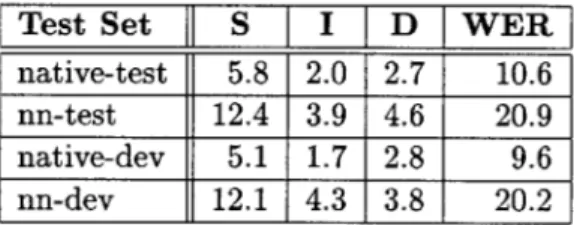
Table 2-4 shows the error rates obtained using the baseline recognizer on the native and non-native test sets. The error rates on the development sets are also shown, as these are used for comparison in subsequent chapters. In all cases, the beam width in the Viterbi
Test Set native-test nn-test native-dev nn-dev S 5.8 12.4 5.1 12.1 I 2.0 3.9 1.7 4.3 D WER 2.7 10.6 4.6 20.9 2.8 9.6 3.8 20.2
Table 2-4: Rates of substitution (S), insertion (I), and deletion (D) and word error rates (WER) obtained with the baseline recognizer on native and non-native sets. Each error rate is a percentage of the number of reference (actual) words in the test set.
search, measured in terms of the score difference between the best- and worst-scoring path considered, is 20. The word transition weight, a parameter controlling the tradeoff between deletions and insertions, is 4. We note the values of these parameters as they will be varied during the course of subsequent experiments.
Chapter 3
Acoustic Modeling
One respect in which native and non-native speakers may differ is in the acoustic features of their speech (e.g., [1]). In other words, when intending to produce the same phone, native and non-native speakers may produce it with different formant frequencies (in the case of sonorants), voice onset times (for stops), durations, and so on. From a speech recognizer's point of view, this difference can affect the behavior of the acoustic models. In this chapter, we investigate the possibility of improving the recognizer's performance on non-native utterances by changing the way in which the acoustic models are trained.
To this end, we created several sets of acoustic models. Section 3.1 compares models trained on the native training set, models trained on the non-native training set, and the baseline models described in Chapter 2. Section 3.2 describes the creation of a combined model by interpolation of the native and non-native models and shows the results of using this model.
3.1
Native and Non-Native Acoustic Models
The native and non-native acoustic models were trained on the native-train and nn-train sets described in Chapter 2. The measurements, label classes, and training procedure were the same as those used to train the baseline models. Table 3-1 shows the performance of recognizers using the native, non-native, and pooled models. All of the recognizers are identical to the baseline recognizer described in Chapter 2, except for the different acoustic models.
As expected, the native models perform better on the native sets than they do on the non-native sets, and the non-native models perform better on the non-native sets than on the native set. The non-native models also perform better on the non-native sets than do the native models. This result is not a foregone conclusion, for two reasons. First, the native models would presumably perform better than the non-native models on non-native test data if the non-native models had sufficiently little training data. This result, therefore,
Native Models Non-Native Models Pooled Models
Test Set S I D WER S I D WER S I D WER
native-dev 5.0 1.6 2.7 9.3 12.9 3.7 5.3 21.8 5.1 1.7 2.8 9.6
nn-dev 13.8 4.9 4.3 23.0 12.6 4.8 3.0 20.4 12.1 4.3 3.8 20.2
native-test 5.4 1.8 2.5 9.7 14.9 3.9 5.1 23.9 5.8 2.0 2.7 10.6
nn-test 14.0 4.4 5.0 23.4 12.8 4.5 4.3 21.7 12.4 3.9 4.6 20.9
Table 3-1: Rates of substitution (S), insertion (I), and deletion (D) and word error rates (WER) for recognizers using the native, non-native, and pooled acoustic models. The sets are the native and non-native development sets (native-dev, and nn-dev, respectively).
provides some assurance that the non-native models are adequately trained. Second, since the non-native models are trained on speakers with many very different accents, it is possible that the resulting models would simply be too broad to accurately model the acoustics of the speech of any one non-native speaker. Therefore, this result also confirms that it is reasonable to model the acoustics of non-native speech with various accents using a single set of models.
The pooled models perform slightly worse on the native sets than do the native models. This indicates that including non-native data in the training set, at least in the proportion we have used, is detrimental to recognition of native speech. However, when testing on non-native speech, the pooled models perform slightly better than the non-native models. This suggests that, although non-native training data is better than native training data for recognition of non-native speech, including native data in the training can be helpful.
3.2
Model Interpolation
While the non-native models perform better on non-native data than do the native models, and the pooled models perform even better by a small amount, there is reason to believe that we could do better than either of these. The improvement we have seen from pooling the native and non-native training data indicates that the recognition of non-native speech can benefit from native training data. However, the pooled training set gives very little weight to the non-native training utterances, since the native utterances outnumber them by a factor of about 12. Intuitively, we would like to give more weight to the non-native training utterances than they receive in the pooled training. It would be undesirable to remove some of the native utterances from the pooled training set to achieve a better balance, since these add to the robustness of the models. One way to achieve the desired weighting is by interpolating the native and non-native models.
3.2.1
Definition
Interpolation of models refers to the weighted averaging of the PDF's of several mod-els to produce a single output. Interpolation is closely related to model aggregation, the averaging of model PDF's using equal weights, which has been shown to improve the per-formance of a recognizer when applied to models from different training runs using the same data [13]. Model interpolation has also been used successfully to combine well-trained context-independent models with less well-trained but more detailed context-dependent models [14]. The case of native and non-native models is similar, in the sense that the native models are better trained but the non-native models are more appropriate for the test population.
Given an observation vector of acoustic features 5, a set of N models
A(F),
2()),- , P , and the corresponding weights w1, w2, - , wN, the interpolated model is defined as:N (S) = EwifA , (3.1) i=1 where Ewi = 1 (3.2) i=1
In our case, there are only two models, Pnat(5) and Pfn(5), where the subscript nat refers to the native model and nn to the non-native one. The expression for the interpolated model is therefore:
P(S) = wnatPnat(S) + Wnn ), (3.3)
where
wnat + wn = 1 (3.4)
3.2.2 Experiments
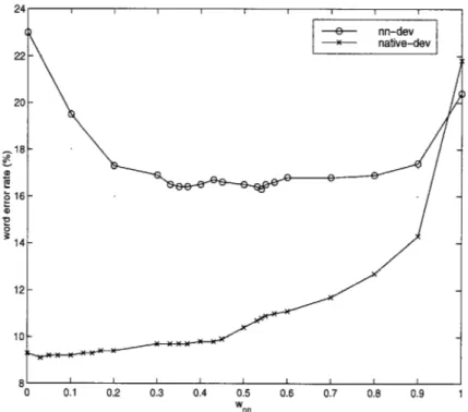
We created a series of interpolated models by varying the relative weights assigned to the native and non-native models. Figure 3-1 shows the results of using these models in recognition experiments on the native and non-native development sets.
As expected, the WER's obtained with won = 0 and wn = 1 are identical to those obtained with native and non-native models alone, respectively. Also as expected, the WER on native-dev displays almost monotonically increasing behavior as the non-native models are given increasingly more weight. The minimum WER, however, does not occur
for Wnn = 0 but for wn = 0.03. With this weighting, the WER is 9.1%, which is a 2.1%
relative error rate reduction (RERR) from the WER obtained with the native models. This may indicate that there is a benefit to interpolating the native and non-native models even for recognition of native speech, although it is not clear that the difference in this experiment
-18
2 16
0
0 0.1 0.2 0.3 0.4 0.5 0.6 0.7 0.8 0.9 1
w
Figure 3-1: Word error rates obtained on native and non-native development sets using interpolated models with varying relative weights.
For nn-dev, the lowest WER, obtained with wn = 0.54, is 16.3%. This is a 20.0% RERR with respect to the non-native models and a 19.3% RERR with respect to the baseline models, indicating that the recognition of non-native speech benefits greatly from the interpolation of native and non-native models.
It is interesting to note that, when testing on nn-dev, almost any amount of interpolation is much better than using either of the individual models. The WER on nn-dev decreases drastically as we go from no interpolation (wan = 0 or 1) to interpolation with wn = 0.2 or 0.9, while varying much less within a large range of won between those values. We also note that there appears to be a local minimum in the WER on nn-dev at won = 0.37-0.35, in addition to the absolute minimum at wnn = 0.54. It is not clear whether or not this can be attributed to statistical variation alone.
Tables 3-2 and 3-3 show the error rates obtained on the non-native and native test sets using interpolated models with wn = 0.54 and won = 0.03, respectively. For nn-test, the WER using the interpolated models is 19.2%, an 8.1% improvement over the pooled models and an 11.5% improvement over the non-native models. For nat-test, using the interpolated models yields a WER of 9.6%, a 9.4% improvement over the pooled models and a 1.0% improvement over the native models.
In order to determine whether these results are the best that we could have obtained on the test sets, we tested the interpolated models on nn-test and nat-test with varying weights, as we did for the development sets. Figure 3-2 shows the results of these
experi-Pooled Models S I D WER 12.4 3.9 4.6 20.9
±
-r
Non-Native Models S I D WER 12.8 4.5 14.3 1 21.7±|
Interpolated S I D 11.5 3.6 4.1Table 3-2: Comparison of error rates on the non-native test set obtained with the baseline models, non-native models, and interpolated models with wn = 0.54
Models D WER 2.7 10.6
II
S11
Native Models I D WER 1.8 2.5 9.7I
Interpolated S I D 5.3 1.8 2.5Table 3-3: Comparison of error rates on the native test set obtained with the baseline models, native models, and interpolated models with wn = 0.03
ments. The lowest WER for nn-test is 18.9%, an improvement of 9.6% over baseline, and occurs at wn = 0.57. For nat-test, the lowest WER is 9.5%, an improvement of 2.1% over the native models alone, and occurs at wn = 0.05.
It is not clear why even the best-performing interpolated model for nn-test produces only about half the improvement that was obtained on nn-dev. This may be due to the large variability in non-native speech; that is, the utterances in the development set may happen to be better modeled by the acoustic models than those in the test set.
Models WER 19.2 S Pooled I 1I 2.0 Models WER 9.6
I
5.4 I0.5 w
Figure 3-2: Word error rates obtained models with varying relative weights.
Chapter 4
Comparison of Native and
Non-Native Lexical Patterns Using
Manual Transcriptions
In this chapter, we investigate the differences between native and non-native patterns of word pronunciation through manual phonetic transcriptions of a small subset of the utter-ances in the JUPITER corpus. We examine the transcriptions both qualitatively, to gain a general impression of the phenomena present, and quantitatively, to measure the frequen-cies of these phenomena. This is an informal investigation, in that only a small number of utterances were transcribed by a single person. However, this type of investigation can provide a general picture of the types of pronunciation differences that exist between native and non-native speakers.
4.1
Manual Transcriptions
The data for this study consist of 100 utterances from 19 native speakers and 96 utterances from 24 non-native speakers, drawn from the JUPITER corpus. Each utterance was
tran-scribed by both listening to portions of the utterance and visually examining a spectrogram of the waveform. The label set for the phonetic transcriptions is based on the one used in the baseline recognizer. However, labels were added as needed to better account for the speech sounds present in the data. This resulted in somewhat different label sets for the native and non-native transcriptions. For example, we found that several of the native speakers tended to use diphthong-like sounds instead of pure vowels. We therefore added several labels corresponding to these sounds. For non-native speakers, we added several short, tense vowels (such as IPA [i], a non-diphthongized, tense, high front vowel), as well as labels for non-native varieties of /r/ and /1/. Several non-standard phones were added for both native and non-native transcriptions, such as IPA [Y] (a lax, rounded, mid-high, mid-front vowel) and IPA [x] (a voiceless velar fricative). The full label sets used for the transcriptions are described in Appendix A. In the discussion and examples of the following